
Numerical Study on the Transport and Settlement of Larval Hippocampus trimaculatus in the Northern South China Sea

Abstract
1. Introduction

2. Materials and Methods
2.1. The Study Time Period and Regional Division
2.2. Configuration of the Ocean Model CROCO
2.3. Configuration of the Biological Model Ichthyop
3. Results
3.1. Simulation of the Ocean Model CROCO
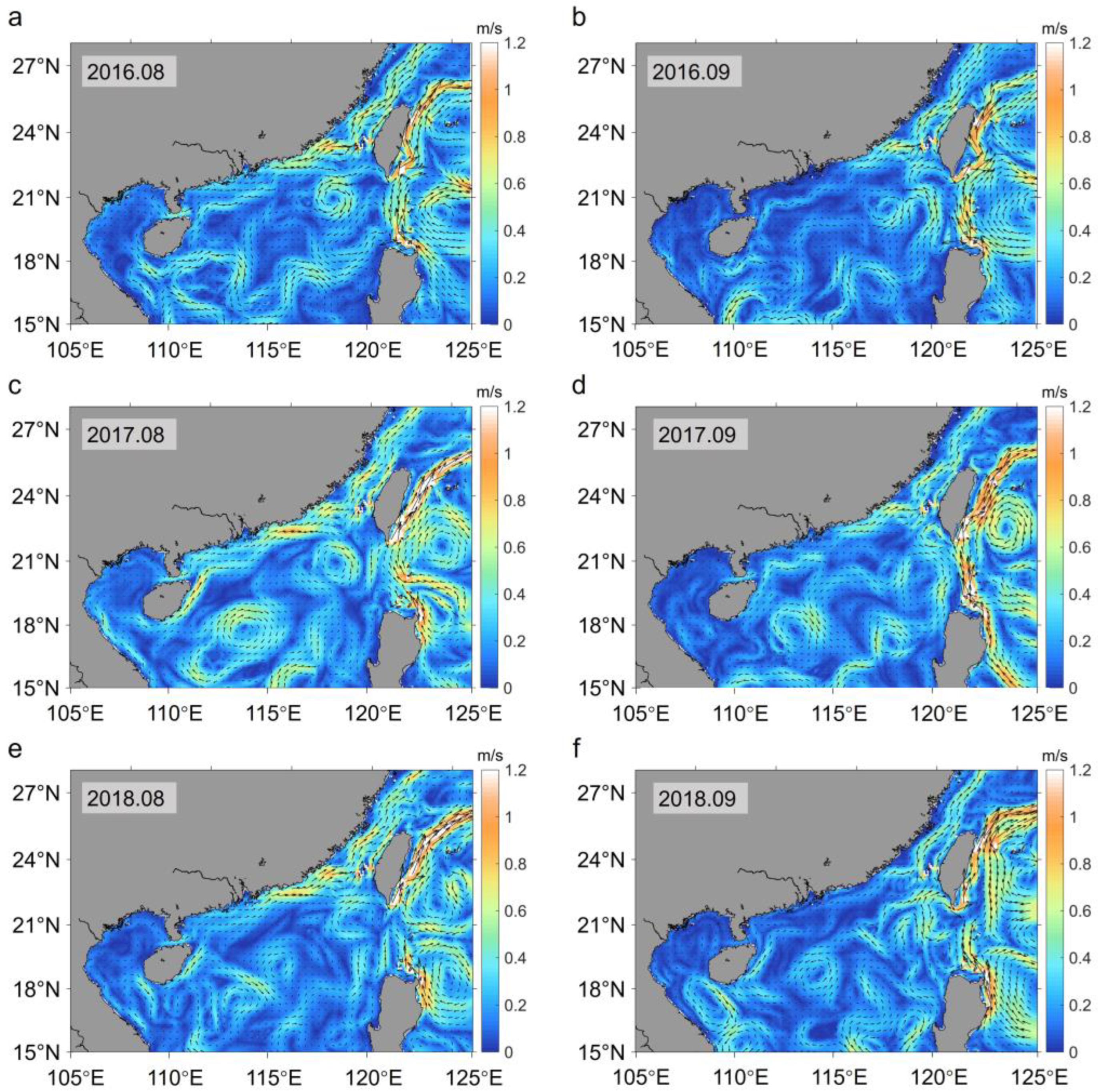
3.1.1. Current Field
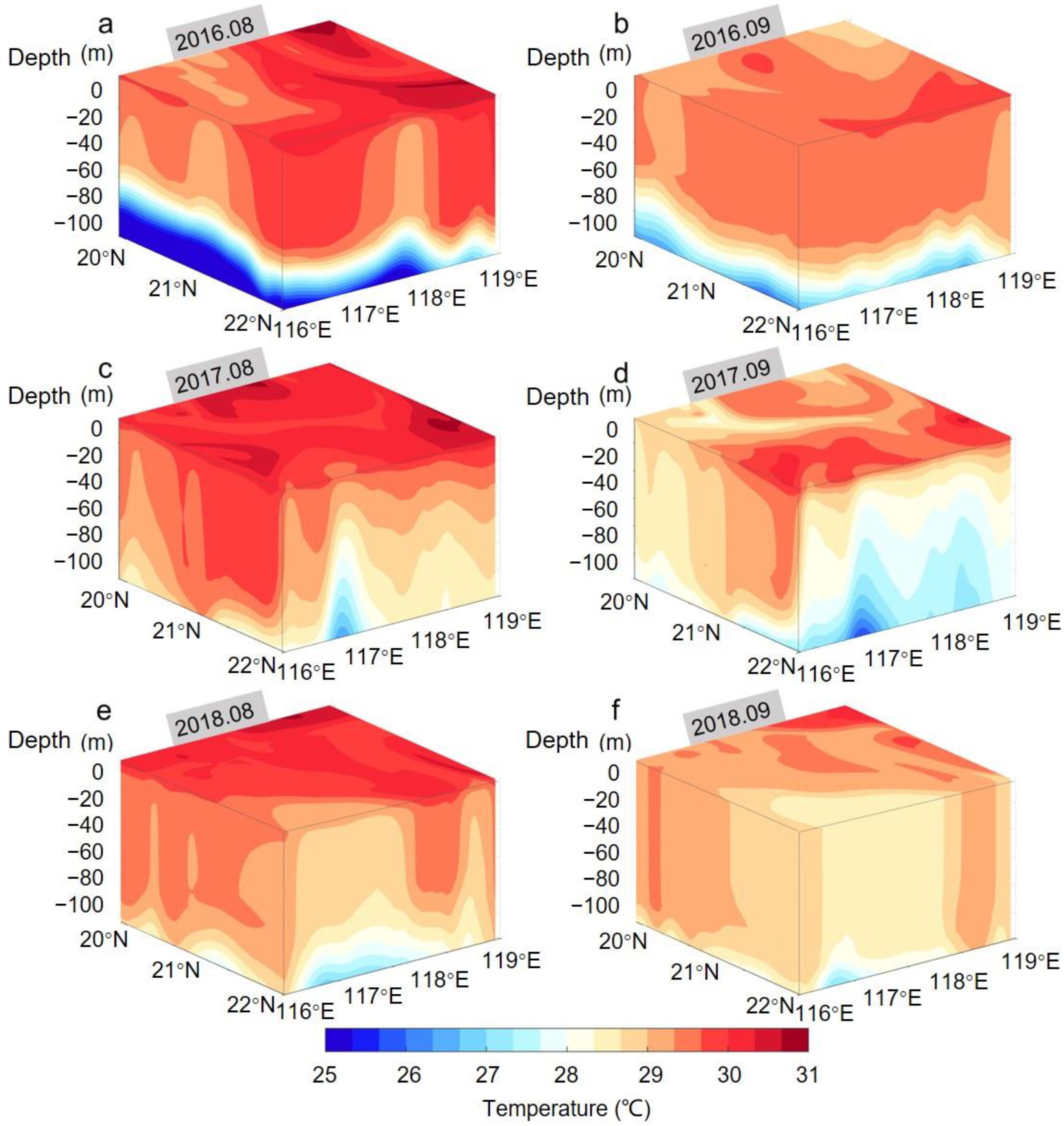
3.1.2. Temperature Field
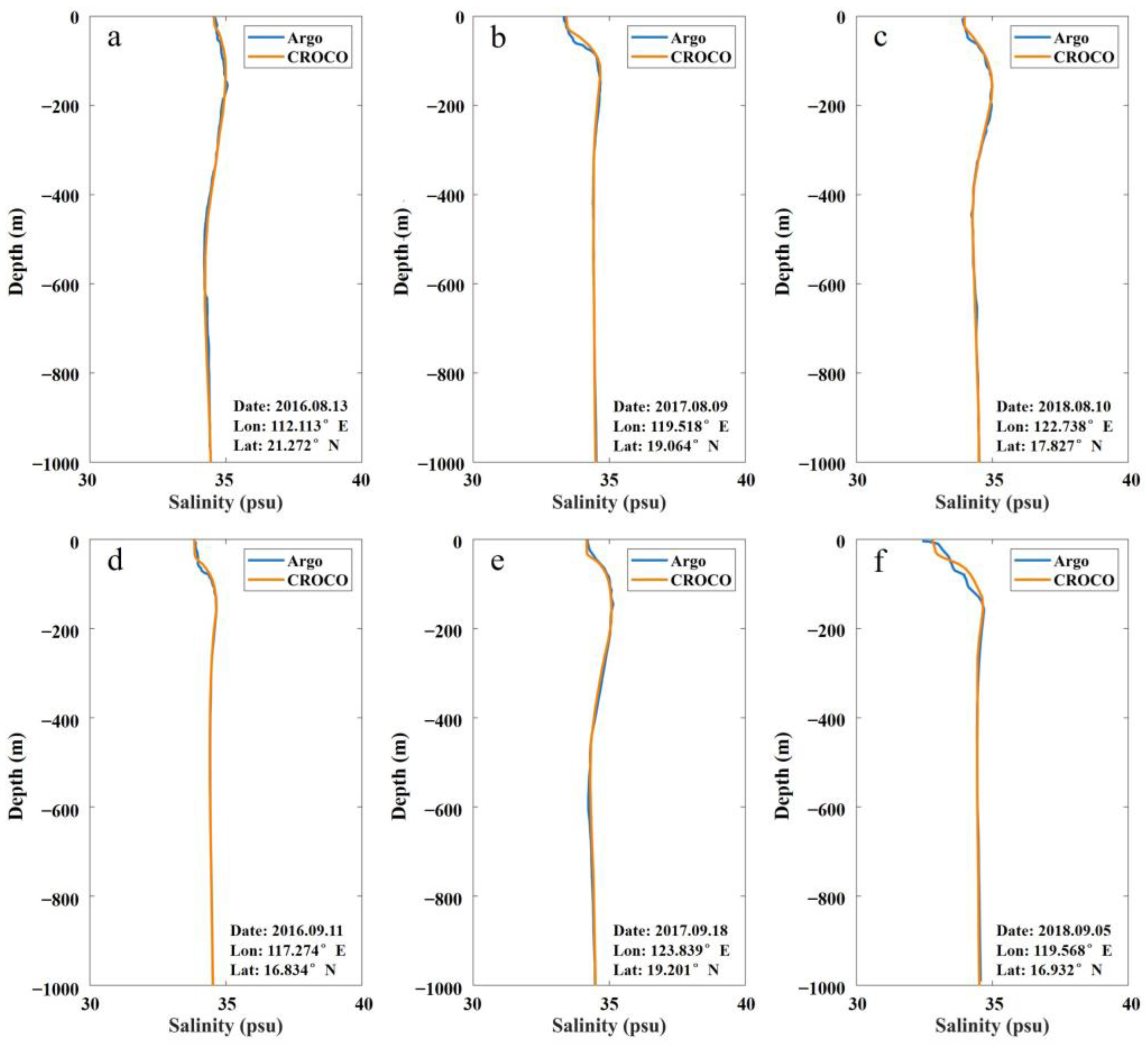
3.1.3. Salinity Field
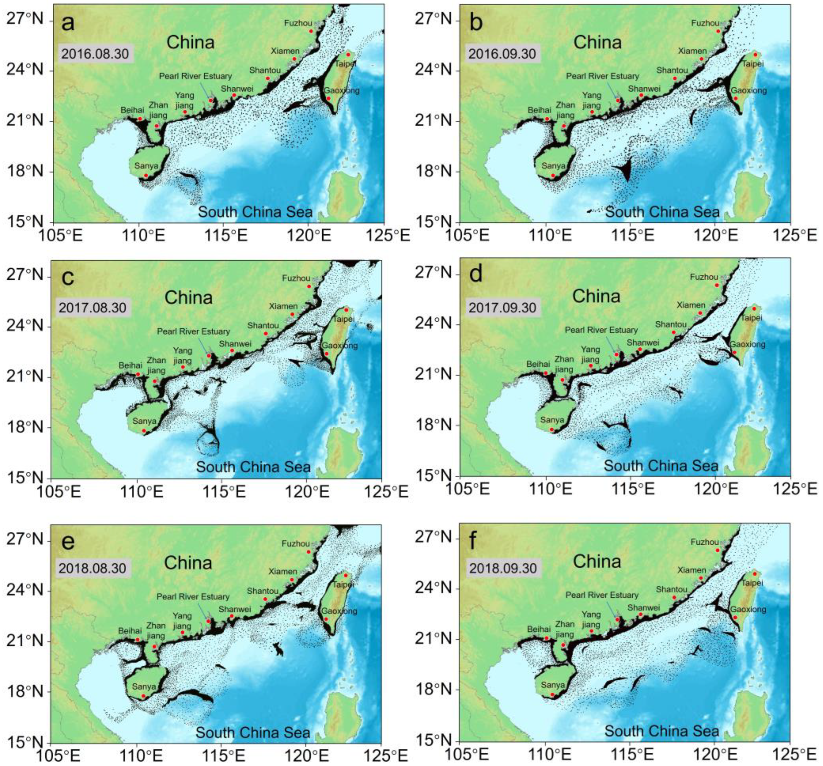
3.2. Simulation of the Biological Model Ichthyop
4. Discussion
4.1. Connectivity
4.2. Transport Distance
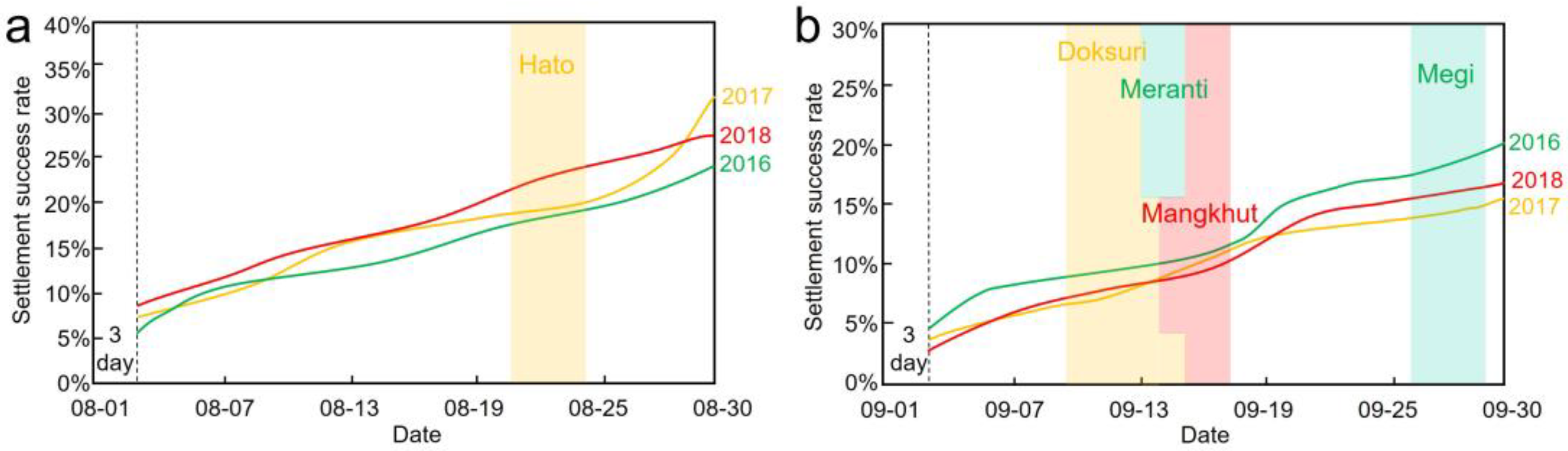
4.3. Settlement Success Rate
4.4. Conservation and Management Recommendations
5. Conclusions and Future Directions
Author Contributions
Funding
Data Availability Statement
Conflicts of Interest
References
- Zhang, X.; Vincent, A.C.J. Integrating Multiple Datasets with Species Distribution Models to Inform Conservation of the Poorly-Recorded Chinese Seahorses. Biol. Conserv. 2017, 211, 161–171. [Google Scholar] [CrossRef]
- Koning, S.; Hoeksema, B.W. Diversity of Seahorse Species (Hippocampus Spp.) in the International Aquarium Trade. Diversity 2021, 13, 187. [Google Scholar] [CrossRef]
- Tiralongo, F.; Baldacconi, R. A Conspicuous Population of the Long-Snouted Seahorse, Hippocampus Guttulatus (Actinopterygii: Syngnathiformes: Syngnathidae), in a Highly Polluted Mediterranean Coastal Lagoon. Acta Ichthyol. Piscat. 2014, 44, 99–104. [Google Scholar] [CrossRef]
- Harasti, D. Declining Seahorse Populations Linked to Loss of Essential Marine Habitats. Mar. Ecol. Prog. Ser. 2016, 546, 173–181. [Google Scholar] [CrossRef]
- Costa, A.B.; Correia, M.; Silva, G.; Lopes, A.F.; Faria, A.M. Performance of the Long-Snouted Seahorse, Hippocampus guttulatus, under Warming Conditions. Front. Mar. Sci. 2023, 10, 1136748. [Google Scholar] [CrossRef]
- Li, N.; Zhang, X.; Liu, X.; Lin, X.; Hu, C.; Chen, J.; Wang, S.; Zhang, D.; Wei, S.; Shi, Q. Chromosome-Scale Genome Assembly of Three-Spotted Seahorse (Hippocampus trimaculatus) with a Unique Karyotype. Sci. Data 2025, 12, 49. [Google Scholar] [CrossRef]
- Norcross, B.L.; Shaw, R.F. Oceanic and Estuarine Transport of Fish Eggs and Larvae: A Review. Trans. Am. Fish. Soc. 1984, 113, 153–165. [Google Scholar] [CrossRef]
- Pineda, J.; Reyns, N. Larval Transport in the Coastal Zone: Biological and Physical Processes. In Evolutionary Ecology of Marine Invertebrate Larvae; Carrier, T., Reitzel, A., Heyland, A., Eds.; Oxford University Press: Oxford, UK, 2017; pp. 145–163. ISBN 978-0-19-878696-2. [Google Scholar]
- Pineda, J.; Hare, J.; Sponaugle, S. Larval Transport and Dispersal in the Coastal Ocean and Consequences for Population Connectivity. Oceanography 2007, 20, 22–39. [Google Scholar] [CrossRef]
- Martínez, S.; Carrillo, L.; Marinone, S.G. Potential Connectivity between Marine Protected Areas in the Mesoamerican Reef for Two Species of Virtual Fish Larvae: Lutjanus analis and Epinephelus striatus. Ecol. Indic. 2019, 102, 10–20. [Google Scholar] [CrossRef]
- Fontoura, L.; D’Agata, S.; Gamoyo, M.; Barneche, D.R.; Luiz, O.J.; Madin, E.M.P.; Eggertsen, L.; Maina, J.M. Protecting Connectivity Promotes Successful Biodiversity and Fisheries Conservation. Science 2022, 375, 336–340. [Google Scholar] [CrossRef]
- Victor, B.C. Larval Settlement and Juvenile Mortality in a Recruitment—Limited Coral Reef Fish Population. Ecol. Monogr. 1986, 56, 145–160. [Google Scholar] [CrossRef]
- Shima, J.S.; Noonburg, E.G.; Swearer, S.E.; Alonzo, S.H.; Osenberg, C.W. Born at the Right Time? A Conceptual Framework Linking Reproduction, Development, and Settlement in Reef Fish. Ecology 2018, 99, 116–126. [Google Scholar] [CrossRef]
- Yip, M.Y.; Lim, A.C.O.; Chong, V.C.; Lawson, J.M.; Foster, S.J. Food and Feeding Habits of the Seahorses Hippocampus spinosissimus and Hippocampus trimaculatus (Malaysia). J. Mar. Biol. Assoc. U. K. 2015, 95, 1033–1040. [Google Scholar] [CrossRef]
- Zhang, X.; Vincent, A.C.J. Predicting Distributions, Habitat Preferences and Associated Conservation Implications for a Genus of Rare Fishes, Seahorses (Hippocampus Spp.). Divers. Distrib. 2018, 24, 1005–1017. [Google Scholar] [CrossRef]
- Li, C.; Olave, M.; Hou, Y.; Qin, G.; Schneider, R.F.; Gao, Z.; Tu, X.; Wang, X.; Qi, F.; Nater, A.; et al. Genome Sequences Reveal Global Dispersal Routes and Suggest Convergent Genetic Adaptations in Seahorse Evolution. Nat. Commun. 2021, 12, 1094. [Google Scholar] [CrossRef]
- Aylesworth, L.; Phoonsawat, R.; Suvanachai, P.; Vincent, A.C.J. Generating Spatial Data for Marine Conservation and Management. Biodivers. Conserv. 2017, 26, 383–399. [Google Scholar] [CrossRef]
- Bosso, L.; Panzuto, R.; Balestrieri, R.; Smeraldo, S.; Chiusano, M.L.; Raffini, F.; Canestrelli, D.; Musco, L.; Gili, C. Integrating Citizen Science and Spatial Ecology to Inform Management and Conservation of the Italian Seahorses. Ecol. Inform. 2024, 79, 102402. [Google Scholar] [CrossRef]
- Zhang, J.; Wang, X.; Jiang, Y.; Chen, Z.; Zhao, X.; Gong, Y.; Ying, Y.; Li, Z.; Kong, X.; Chen, G.; et al. Species Composition and Biomass Density of Mesopelagic Nekton of the South China Sea Continental Slope. Deep Sea Res. Part. II Top. Stud. Oceanogr. 2019, 167, 105–120. [Google Scholar] [CrossRef]
- Huang, D.; Zhang, X.; Jiang, Z.; Zhang, J.; Arbi, I.; Jiang, X.; Huang, X.; Zhang, W. Seasonal Fluctuations of Ichthyoplankton Assemblage in the Northeastern S Outh C Hina S Ea Influenced by the K Uroshio Intrusion. J. Geophys. Res. Oceans 2017, 122, 7253–7266. [Google Scholar] [CrossRef]
- Huang, F.; Chen, Y.; Wang, K.; Liang, J.; Liu, Q.; Xiong, Z.; Lan, F.; Yin, K. Effects of Topography on Nutrient Variations in the Western South China Sea. J. Geophys. Res. Oceans 2024, 129, e2024JC021006. [Google Scholar] [CrossRef]
- Liu, J.; Dai, J.; Xu, D.; Wang, J.; Yuan, Y. Seasonal and Interannual Variability in Coastal Circulations in the Northern South China Sea. Water 2018, 10, 520. [Google Scholar] [CrossRef]
- Chen, J.; Hu, Z. Seasonal Variability in Spatial Patterns of Sea Surface Cold- and Warm Fronts over the Continental Shelf of the Northern South China Sea. Front. Mar. Sci. 2023, 9, 1100772. [Google Scholar] [CrossRef]
- Shu, Y.; Xue, H.; Wang, D.; Xie, Q.; Chen, J.; Li, J.; Chen, R.; He, Y.; Li, D. Observed Evidence of the Anomalous South China Sea western Boundary Current during the Summers of 2010 and 2011. J. Geophys. Res. Oceans 2016, 121, 1145–1159. [Google Scholar] [CrossRef]
- Guo, Z.; Wang, S.; Cao, A.; Xie, J.; Song, J.; Guo, X. Refraction of the M2 Internal Tides by Mesoscale Eddies in the South China Sea. Deep Sea Res. Part. I Oceanogr. Res. Pap. 2023, 192, 103946. [Google Scholar] [CrossRef]
- Fang, W.-P.; Wu, D.-R.; Zheng, Z.-W.; Gopalakrishnan, G.; Ho, C.-R.; Zheng, Q.; Huang, C.-F.; Ho, H.; Weng, M.-C. Impacts of the Kuroshio Intrusion through the Luzon Strait on the Local Precipitation Anomaly. Remote Sens. 2021, 13, 1113. [Google Scholar] [CrossRef]
- Liu, S.; Zuo, J.; Shu, Y.; Ji, Q.; Cai, Y.; Yao, J. The Intensified Trend of Coastal Upwelling in the South China Sea during 1982–2020. Front. Mar. Sci. 2023, 10, 1084189. [Google Scholar] [CrossRef]
- Chen, W.; Tong, Y.; Li, W.; Ding, Y.; Li, J.; Wang, W.; Shi, P. Interannual Variations in the Summer Coastal Upwelling in the Northeastern South China Sea. Remote Sens. 2024, 16, 1282. [Google Scholar] [CrossRef]
- Li, D.; Gan, J.; Hui, R.; Liu, Z.; Yu, L.; Lu, Z.; Dai, M. Vortex and Biogeochemical Dynamics for the Hypoxia Formation Within the Coastal Transition Zone off the Pearl River Estuary. J. Geophys. Res. Oceans 2020, 125, e2020JC016178. [Google Scholar] [CrossRef]
- Grimm, V.; Ayllón, D.; Railsback, S.F. Next-Generation Individual-Based Models Integrate Biodiversity and Ecosystems: Yes We Can, and Yes We Must. Ecosystems 2017, 20, 229–236. [Google Scholar] [CrossRef]
- Zeller, K.; Wattles, D.; Bauder, J.; DeStefano, S. Forecasting Seasonal Habitat Connectivity in a Developing Landscape. Land 2020, 9, 233. [Google Scholar] [CrossRef]
- Guo, C.; Ito, S.; Kamimura, Y.; Xiu, P. Evaluating the Influence of Environmental Factors on the Early Life History Growth of Chub Mackerel (Scomber japonicus) Using a Growth and Migration Model. Prog. Oceanogr. 2022, 206, 102821. [Google Scholar] [CrossRef]
- Mayorga-Adame, C.G.; Batchelder, H.P.; Spitz, Y.H. Modeling Larval Connectivity of Coral Reef Organisms in the Kenya-Tanzania Region. Front. Mar. Sci. 2017, 4, 92. [Google Scholar] [CrossRef]
- Shu, Y.; Wang, Q.; Zu, T. Progress on Shelf and Slope Circulation in the Northern South China Sea. Sci. China Earth Sci. 2018, 61, 560–571. [Google Scholar] [CrossRef]
- Murugan, A.; Dhanya, S.; Sreepada, R.A.; Rajagopal, S.; Balasubramanian, T. Breeding and Mass-Scale Rearing of Three Spotted Seahorse, Hippocampus trimaculatus Leach under Captive Conditions. Aquaculture 2009, 290, 87–96. [Google Scholar] [CrossRef]
- Zheng, X.; Sun, R.; Dai, Z.; He, L.; Li, C. Distribution and Risk Assessment of Microplastics in Typical Ecosystems in the South China Sea. Sci. Total Environ. 2023, 883, 163678. [Google Scholar] [CrossRef] [PubMed]
- Camins, E.; Stanton, L.M.; Correia, M.; Foster, S.J.; Koldewey, H.J.; Vincent, A.C.J. Advances in Life-history Knowledge for 35 Seahorse Species from Community Science. J. Fish. Biol. 2024, 104, 1548–1565. [Google Scholar] [CrossRef]
- Guo, Z.; Cao, A.; Wang, S. Influence of Remote Internal Tides on the Locally Generated Internal Tides upon the Continental Slope in the South China Sea. J. Mar. Sci. Eng. 2021, 9, 1268. [Google Scholar] [CrossRef]
- Zeng, X.; Bracco, A.; Tagklis, F. Dynamical Impact of the Mekong River Plume in the South China Sea. J. Geophys. Res. Oceans 2022, 127, e2021JC017572. [Google Scholar] [CrossRef]
- Li, M.; He, Y.; Liu, G. Atmospheric and Oceanic Responses to Super Typhoon Mangkhut in the South China Sea: A Coupled CROCO-WRF Simulation. J. Ocean. Limnol. 2023, 41, 1369–1388. [Google Scholar] [CrossRef]
- Gnedin, N.Y.; Semenov, V.A.; Kravtsov, A.V. Enforcing the Courant–Friedrichs–Lewy Condition in Explicitly Conservative Local Time Stepping Schemes. J. Comput. Phys. 2018, 359, 93–105. [Google Scholar] [CrossRef]
- Sinhababu, A.; Ayyalasomayajula, S. An Improved Dealiasing Scheme for the Fourth-order Runge-Kutta Method: Formulation, Accuracy and Efficiency Analysis. Int. J. Numer. Methods Fluids 2021, 93, 559–589. [Google Scholar] [CrossRef]
- Sheng, J.; Lin, Q.; Chen, Q.; Gao, Y.; Shen, L.; Lu, J. Effects of Food, Temperature and Light Intensity on the Feeding Behavior of Three-Spot Juvenile Seahorses, Hippocampus trimaculatus Leach. Aquaculture 2006, 256, 596–607. [Google Scholar] [CrossRef]
- Von Schuckmann, K.; Le Traon, P.-Y.; Alvarez-Fanjul, E.; Axell, L.; Balmaseda, M.; Breivik, L.-A.; Brewin, R.J.W.; Bricaud, C.; Drevillon, M.; Drillet, Y.; et al. The Copernicus Marine Environment Monitoring Service Ocean State Report. J. Oper. Oceanogr. 2016, 9, s235–s320. [Google Scholar] [CrossRef]
- Xian, P.; Ji, B.; Bian, S.; Zong, J.; Zhang, T. Influence of Differences in the Density of Seawater on the Measurement of the Underwater Gravity Gradient. Sensors 2023, 23, 714. [Google Scholar] [CrossRef]
- Park, Y.-G.; Choi, A. Long-Term Changes of South China Sea Surface Temperatures in Winter and Summer. Cont. Shelf Res. 2017, 143, 185–193. [Google Scholar] [CrossRef]
- Xiao, F.; Wang, D.; Zeng, L.; Liu, Q.-Y.; Zhou, W. Contrasting Changes in the Sea Surface Temperature and Upper Ocean Heat Content in the South China Sea during Recent Decades. Clim. Dyn. 2019, 53, 1597–1612. [Google Scholar] [CrossRef]
- Zavala-Garay, J.; Rogowski, P.; Wilkin, J.; Terrill, E.; Shearman, R.K.; Tran, L.H. An Integral View of the Gulf of Tonkin Seasonal Dynamics. J. Geophys. Res. Oceans 2022, 127, e2021JC018125. [Google Scholar] [CrossRef]
- Zhou, X.; Jin, G.; Li, J.; Song, Z.; Zhang, S.; Chen, C.; Huang, C.; Chen, F.; Zhu, Q.; Meng, Y. Effects of Typhoon Mujigae on the Biogeochemistry and Ecology of a Semi-Enclosed Bay in the Northern South China Sea. J. Geophys. Res. Biogeosciences 2021, 126, e2020JG006031. [Google Scholar] [CrossRef]
- Lu, X.; Yu, H.; Ying, M.; Zhao, B.; Zhang, S.; Lin, L.; Bai, L.; Wan, R. Western North Pacific Tropical Cyclone Database Created by the China Meteorological Administration. Adv. Atmos. Sci. 2021, 38, 690–699. [Google Scholar] [CrossRef]
- Jarić, I.; Crowley, S.L.; Veríssimo, D.; Jeschke, J.M. Flagship Events and Biodiversity Conservation. Trends Ecol. Evol. 2024, 39, 106–108. [Google Scholar] [CrossRef]
- Shokri, M.R.; Gladstone, W.; Jelbart, J. The Effectiveness of Seahorses and Pipefish (Pisces: Syngnathidae) as a Flagship Group to Evaluate the Conservation Value of Estuarine Seagrass Beds. Aquat. Conserv. 2009, 19, 588–595. [Google Scholar] [CrossRef]
- Maestro, M.; Pérez-Cayeiro, M.L.; Chica-Ruiz, J.A.; Reyes, H. Marine Protected Areas in the 21st Century: Current Situation and Trends. Ocean. Coast. Manag. 2019, 171, 28–36. [Google Scholar] [CrossRef]
- Stocks, A.P.; Foster, S.J.; Bat, N.K.; Ha, N.M.; Vincent, A.C.J. Local Fishers’ Knowledge of Target and Incidental Seahorse Catch in Southern Vietnam. Hum. Ecol. 2019, 47, 397–408. [Google Scholar] [CrossRef]
- Anticamara, J.A.; Go, K.T.B. Impacts of Super-Typhoon Yolanda on Philippine Reefs and Communities. Reg. Environ. Change 2017, 17, 703–713. [Google Scholar] [CrossRef]


| Variable | Value and Descriptions |
|---|---|
| Start and end time | August 1 and September 30 (2016–2018) |
| Transport duration | 30 days, based on the body size |
| Computational time step | 600 s, to satisfy the CFL condition |
| Recording frequency | 6 h |
| Numerical scheme of advection process | Runge–Kutta 4, reducing errors |
| Scheme of turbulent dissipation | 1 × 10⁻⁹ m2/s3 |
| Release depth | Uniform release at depths of 0–50 m |
| DVM behavior | 07:30–19:30 deeper; 19:30–07:30 shallower |
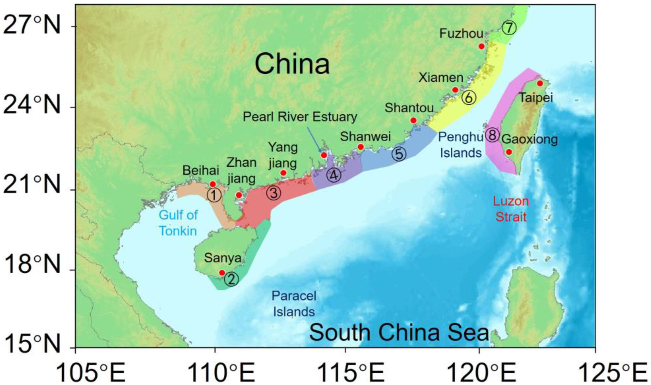
| Release regions | Regions 1–5 and 8, as shown in Figure 2 |
| Release time | August 1 and September 1, 7:30 AM |
| Release number | 4000/release region |
| Buoyancy | , as shown in Equation (1) |
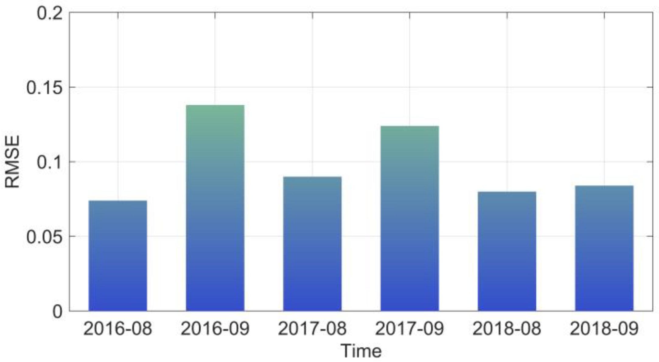
| Date | Mean | STD | RMSE | CC | Location | |||
|---|---|---|---|---|---|---|---|---|
| Argo | CROCO | Argo | CROCO | Latitude (° N) | Longitude (° E) | |||
| 20160813 | 34.7 | 34.6 | 0.1 | 0.2 | 0.3 | 99.8% | 21.272 | 112.113 |
| 20160911 | 34.1 | 34.0 | 0.2 | 0.2 | 0.4 | 99.9% | 16.834 | 117.274 |
| 20170809 | 33.8 | 33.9 | 0.4 | 0.3 | 0.8 | 99.6% | 19.064 | 119.518 |
| 20170918 | 34.4 | 34.3 | 0.3 | 0.3 | 0.5 | 99.8% | 19.201 | 123.839 |
| 20180810 | 34.3 | 34.1 | 0.3 | 0.2 | 0.3 | 99.7% | 17.827 | 122.738 |
| 20180905 | 33.5 | 33.1 | 0.4 | 0.5 | 0.9 | 99.6% | 16.932 | 119.568 |
Disclaimer/Publisher’s Note: The statements, opinions and data contained in all publications are solely those of the individual author(s) and contributor(s) and not of MDPI and/or the editor(s). MDPI and/or the editor(s) disclaim responsibility for any injury to people or property resulting from any ideas, methods, instructions or products referred to in the content. |
© 2025 by the authors. Licensee MDPI, Basel, Switzerland. This article is an open access article distributed under the terms and conditions of the Creative Commons Attribution (CC BY) license (https://creativecommons.org/licenses/by/4.0/).
Share and Cite
Zhang, C.; Deng, Z. Numerical Study on the Transport and Settlement of Larval Hippocampus trimaculatus in the Northern South China Sea. J. Mar. Sci. Eng. 2025, 13, 900. https://doi.org/10.3390/jmse13050900
Zhang C, Deng Z. Numerical Study on the Transport and Settlement of Larval Hippocampus trimaculatus in the Northern South China Sea. Journal of Marine Science and Engineering. 2025; 13(5):900. https://doi.org/10.3390/jmse13050900
Chicago/Turabian StyleZhang, Chi, and Zengan Deng. 2025. "Numerical Study on the Transport and Settlement of Larval Hippocampus trimaculatus in the Northern South China Sea" Journal of Marine Science and Engineering 13, no. 5: 900. https://doi.org/10.3390/jmse13050900
APA StyleZhang, C., & Deng, Z. (2025). Numerical Study on the Transport and Settlement of Larval Hippocampus trimaculatus in the Northern South China Sea. Journal of Marine Science and Engineering, 13(5), 900. https://doi.org/10.3390/jmse13050900