A Parametric Study on the Effect of Blade Configuration in a Double-Stage Savonius Hydrokinetic Turbine


Abstract
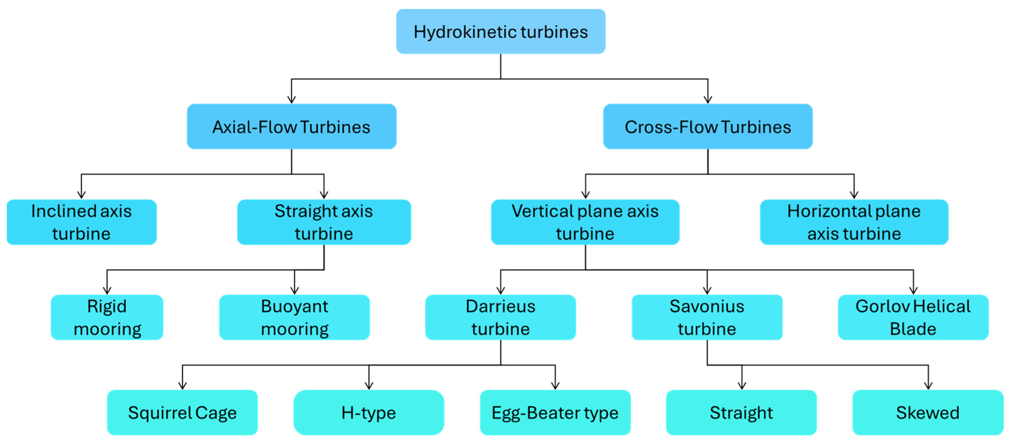
1. Introduction
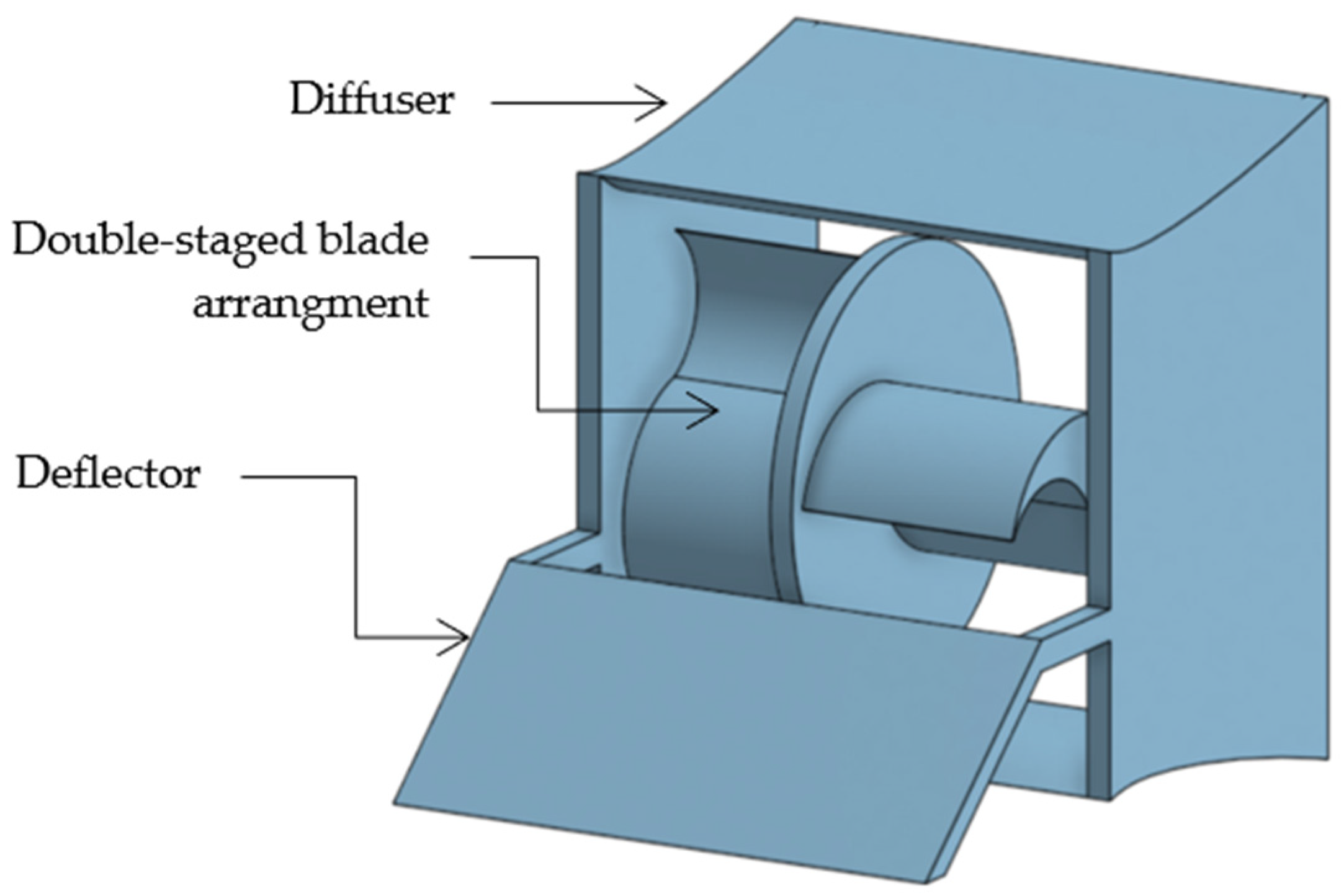
2. The Hydrokinetic Turbine Model
2.1. Single-Stage Hydrokinetic Turbine (HKT) for Numerical Setup Validation
2.2. Double-Stage Hydrokinetic Turbine (HKT) Configurations for Performance Analysis
3. Numerical Methodology
3.1. Governing Equations and Solver Setup
- is the mean velocity vector;
- is the fluid density;
- is the fluid pressure;
- is the dynamic viscosity;
- g is gravitational acceleration.
- are the turbulent Prandtl numbers for k and ;
- is the turbulent kinetic energy (TKE) due to mean velocity shear;
- is the TKE due to buoyancy;
- are the user-defined source term.
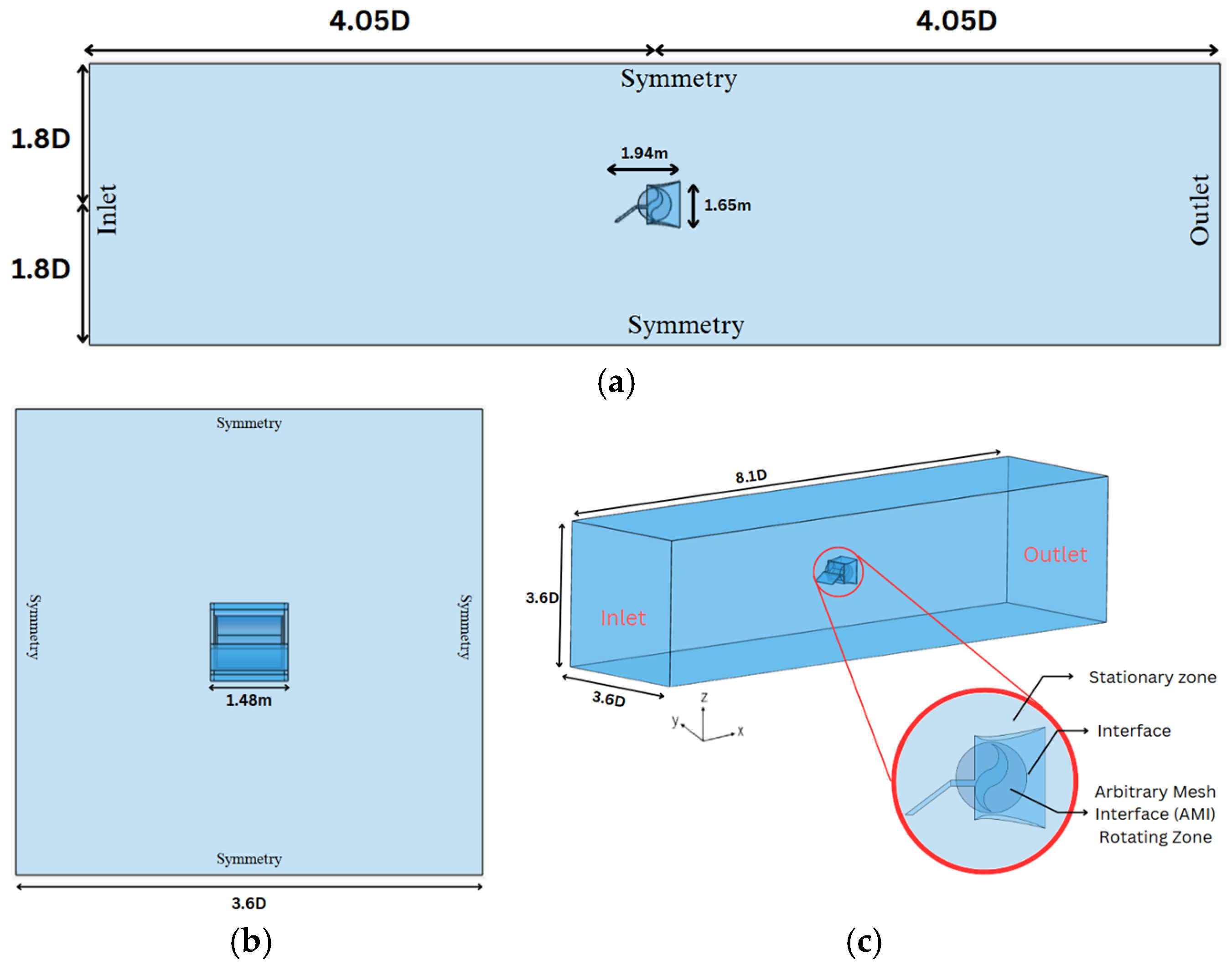
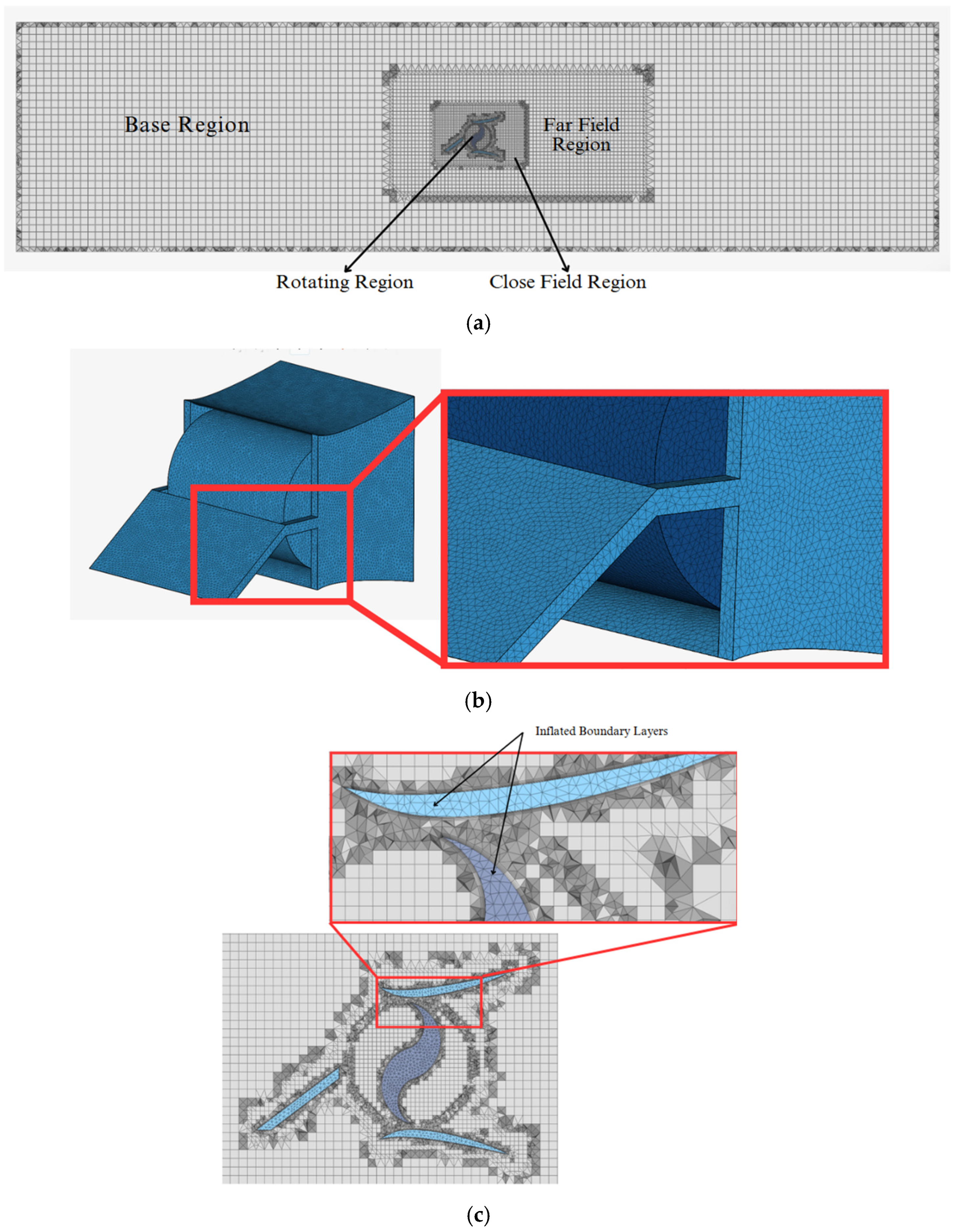
3.2. Computational Domain and Boundary Conditions
3.3. Simulation Conditions and TSR Matrix
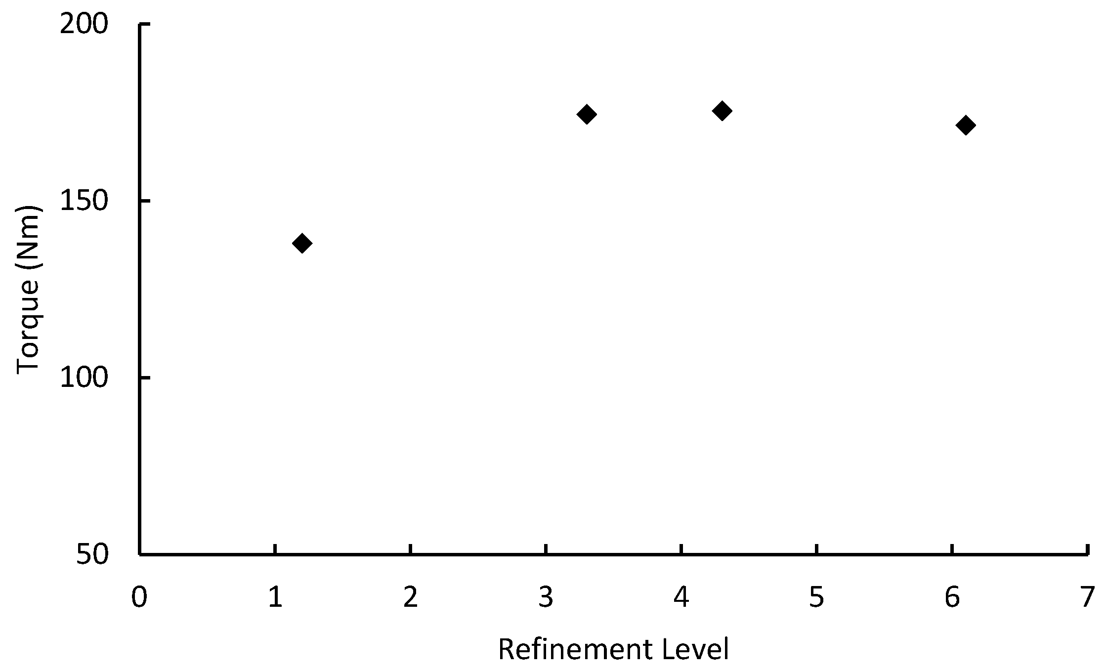
3.4. Mesh Density Analysis
3.5. Time-Step Analysis
3.6. Performance Parameters
- ω is the rotational speed (rad/s);
- R is the rotor radius (m);
- U is the free-stream velocity (m/s).
- Poutput is the power output;
- Pfluid is the power available in the fluid;
- τ is the average peak torque (Nm);
- A is the turbine swept area (m2).
3.7. Model Validation
4. Results and Discussion
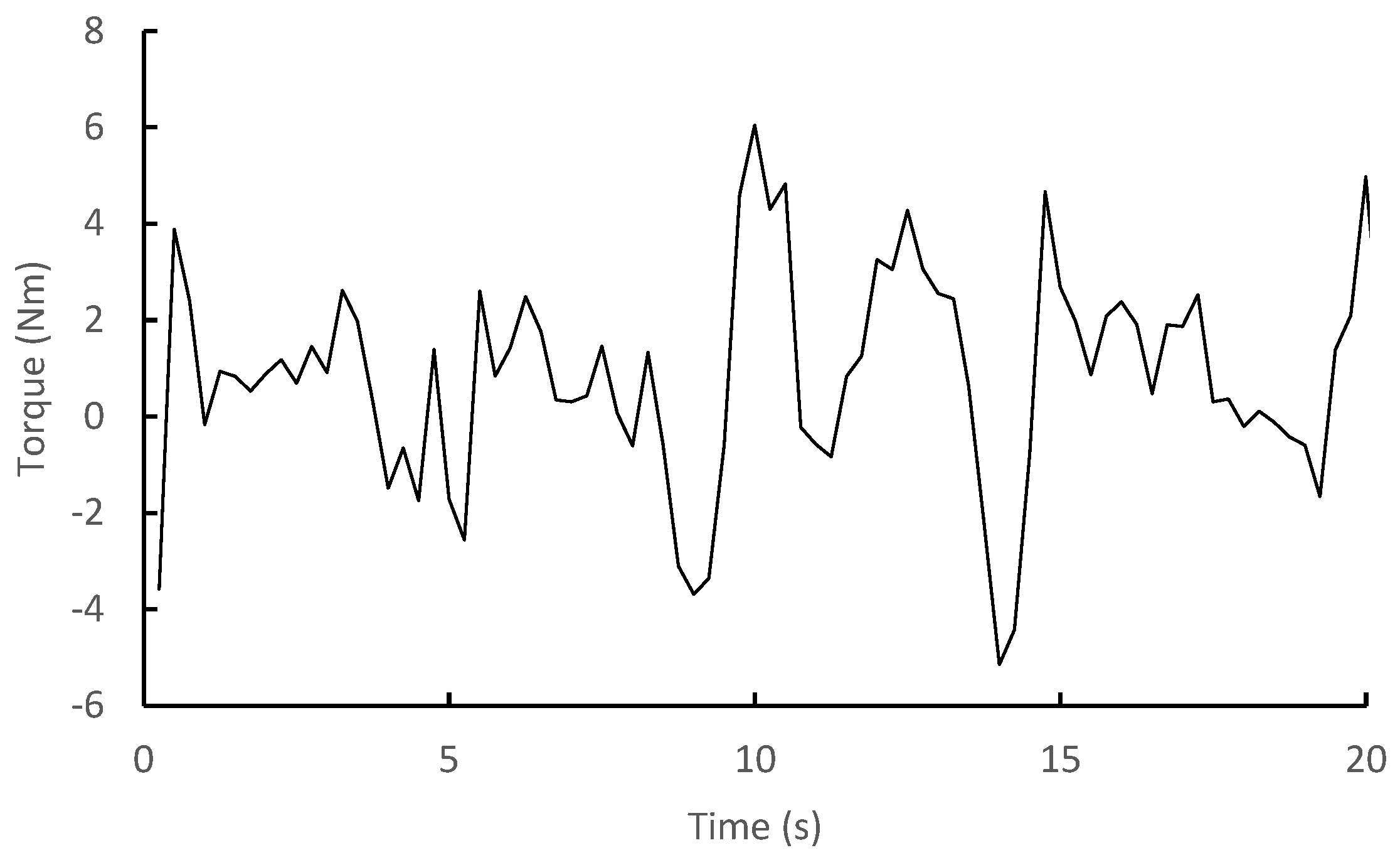
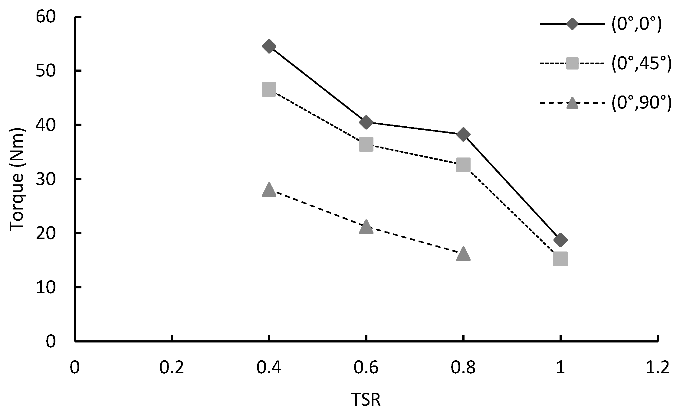
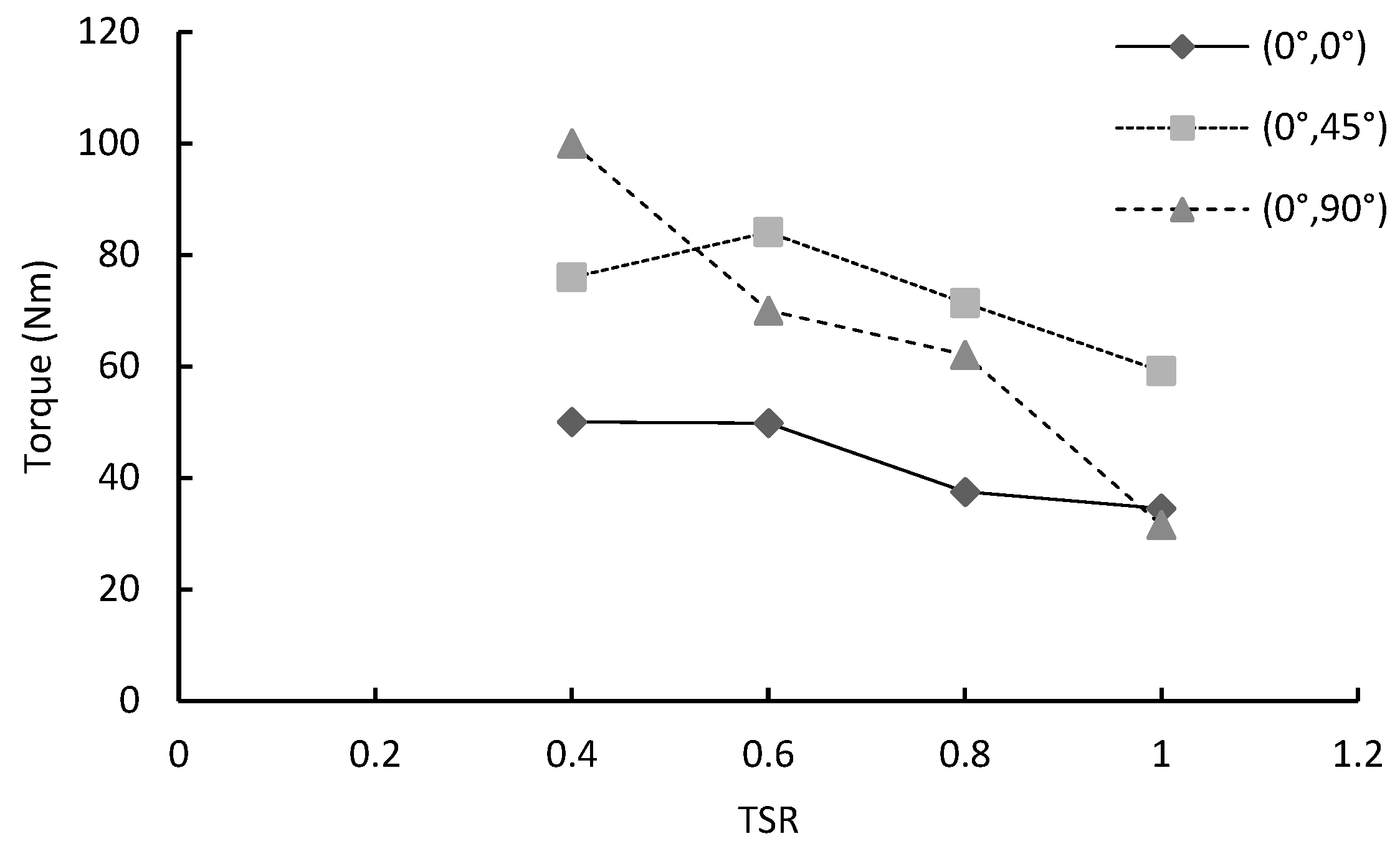
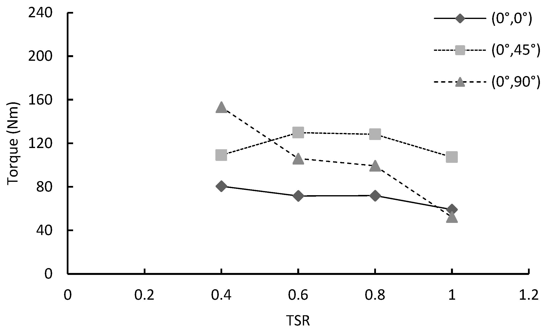
4.1. Effects of Double-Stage Turbine’s Blade Configurations on the Torque Performance
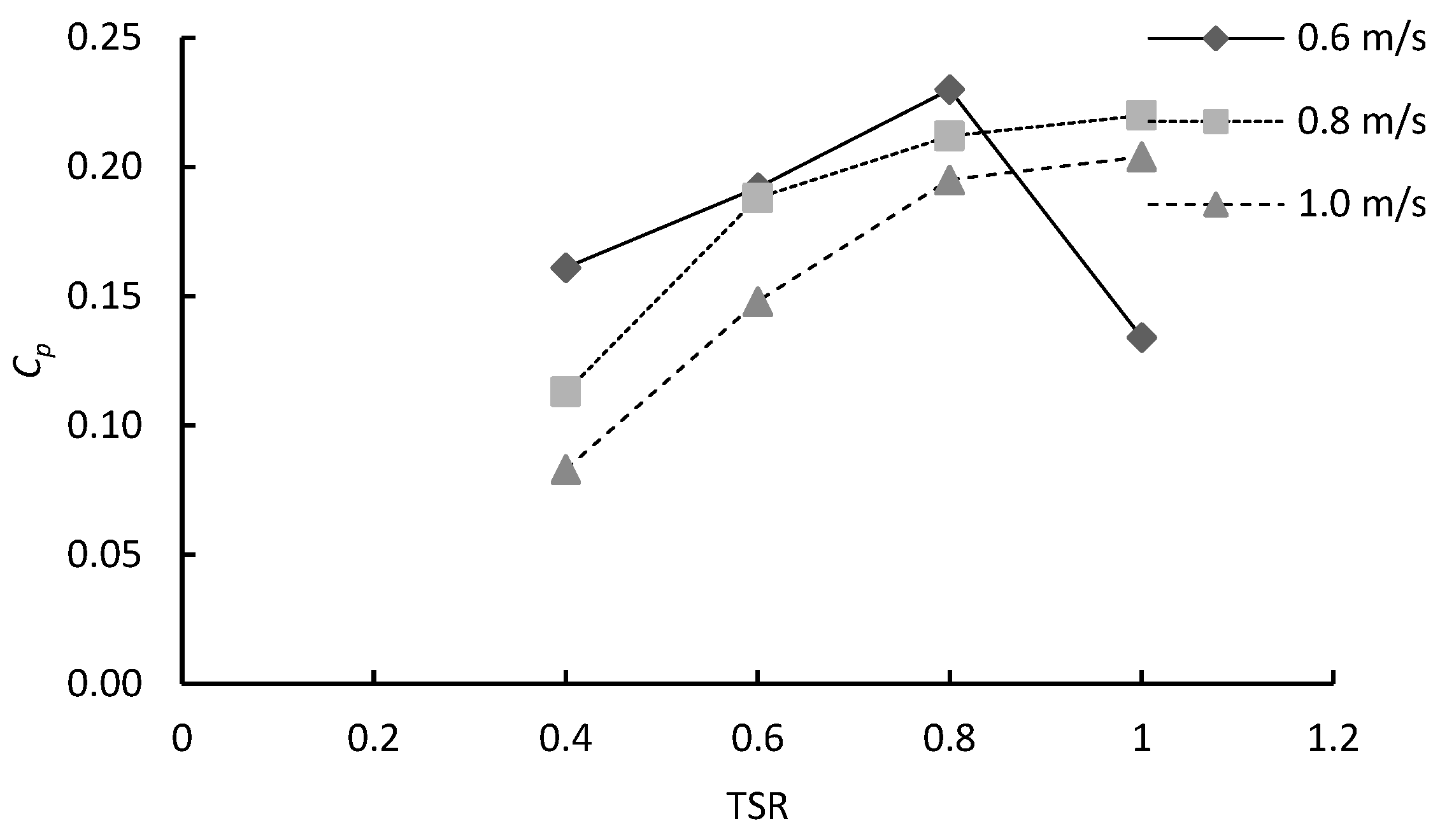
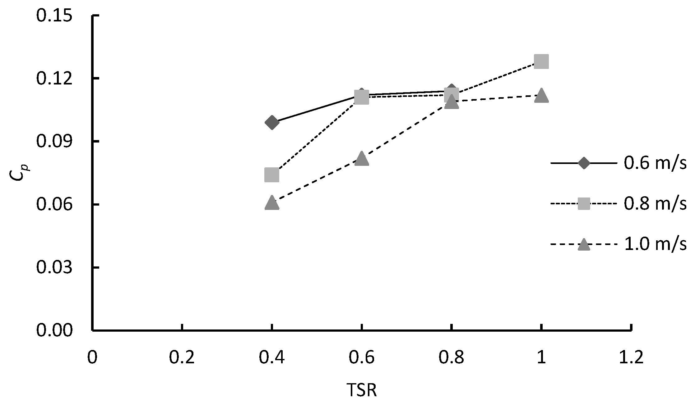
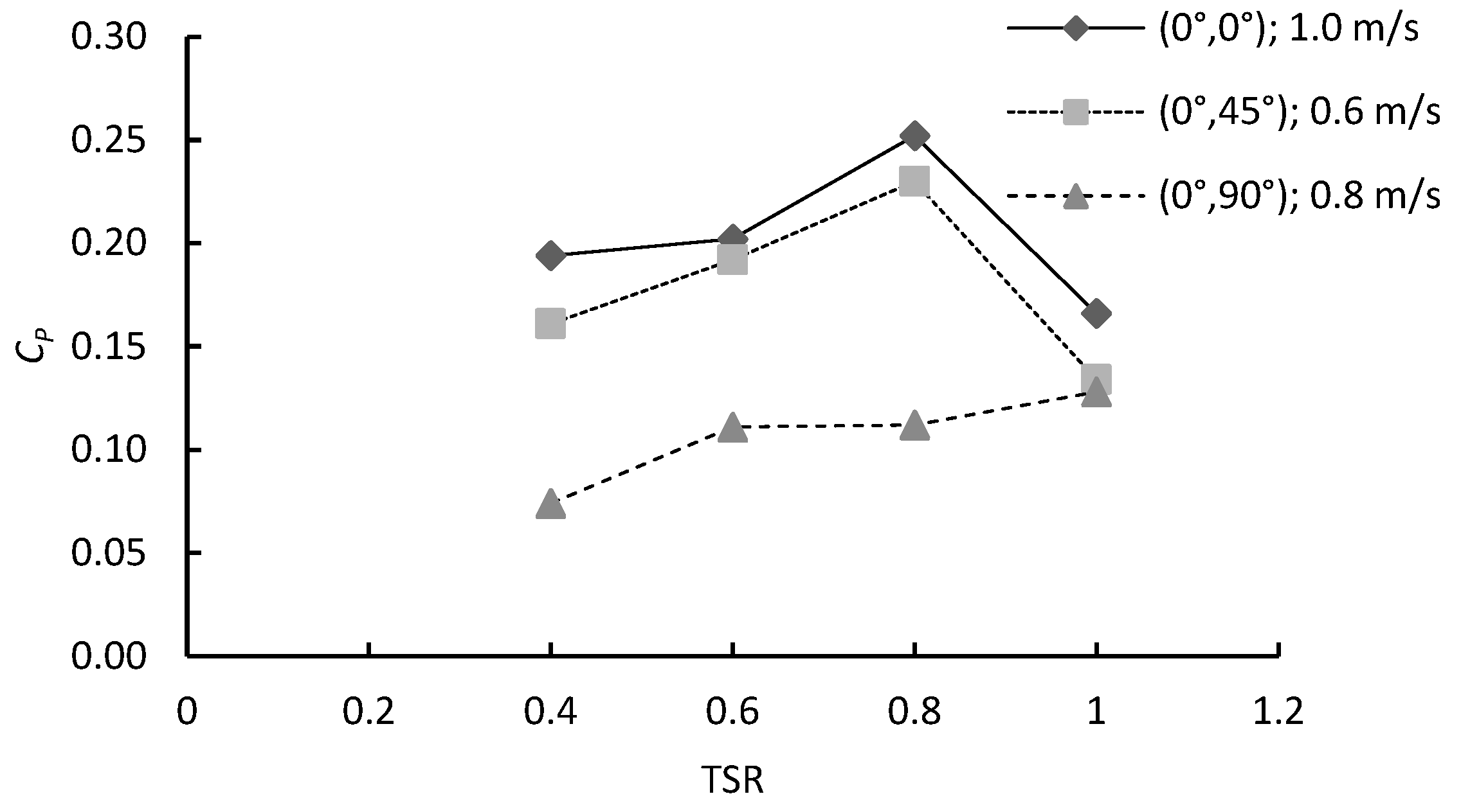
4.2. Effects of Blade Configuration on Power Coefficient of a Double-Stage Hydrokinetic Turbine
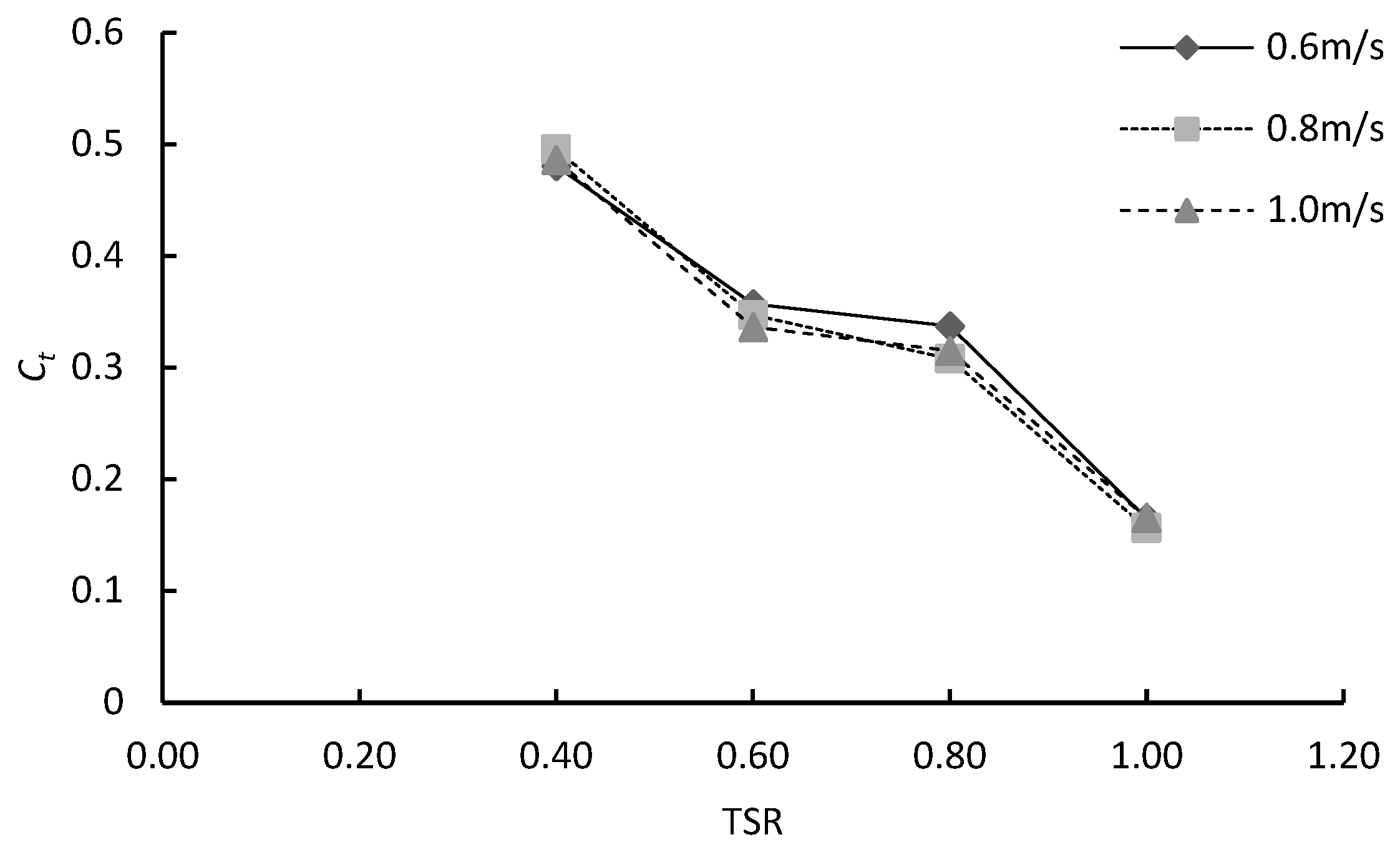
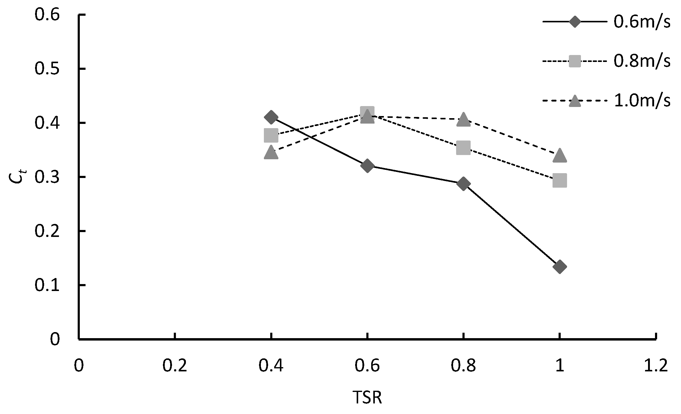
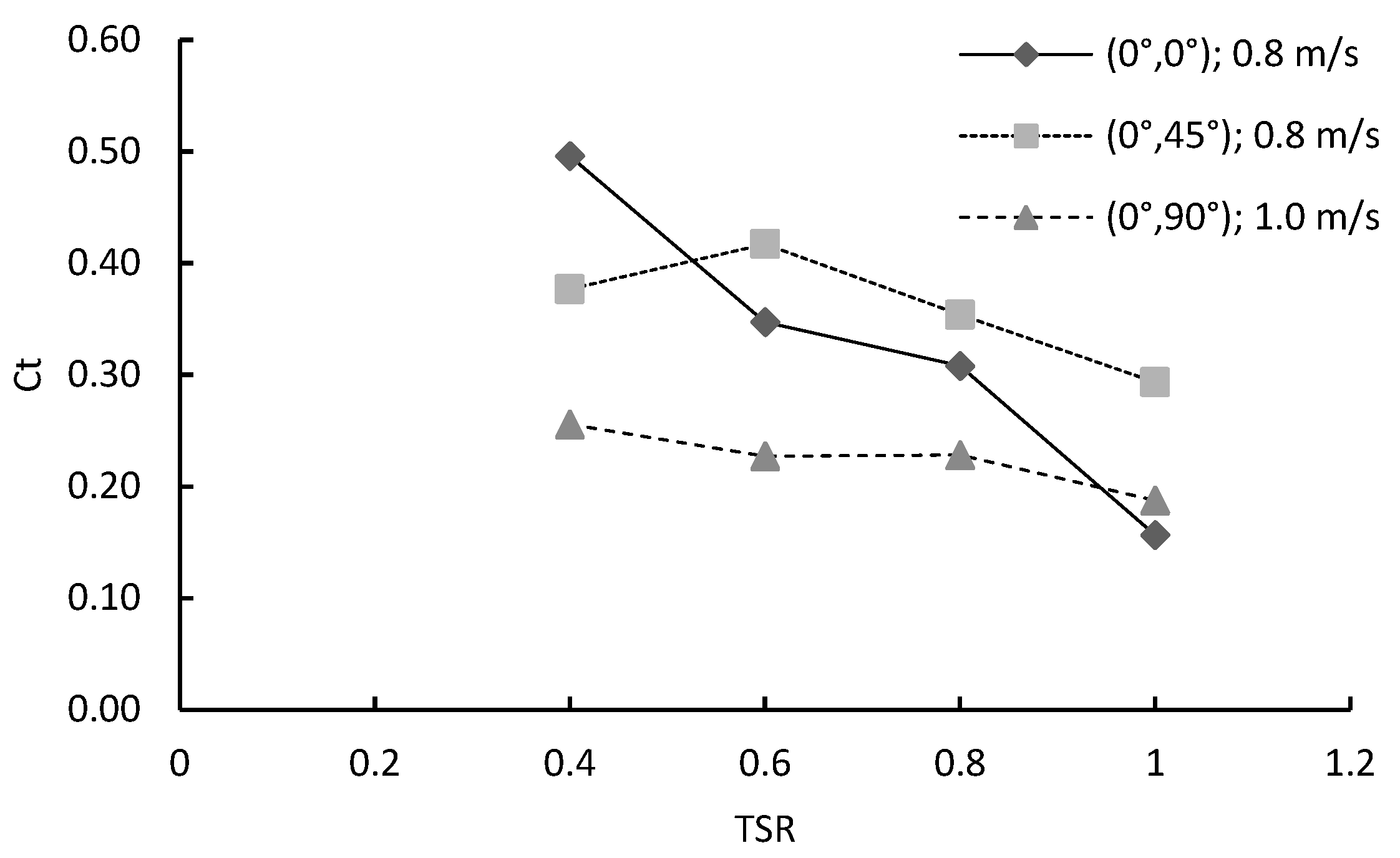
4.3. Effects of Blade Configuration on Torque Coefficient of a Double-Stage Hydrokinetic Turbine
5. Conclusions
- The (0°, 0°) blade configuration achieved the highest Cp of 0.252 at TSR 0.8 and 1.0 m/s. It maintained strong performance at higher flow conditions;
- The (0°, 45°) configuration recorded the highest Cp of 0.230 at 0.6 m/s and TSR 0.8, showing its effectiveness in lower flow conditions;
- The (0°, 90°) configuration consistently produced the lowest Cp values across all velocities;
- Torque output decreased with increasing TSR for all cases. The (0°, 0°) configuration shows higher torque at high TSRs, while the (0°, 45°) configuration performed effectively at mid-TSRs. The (0°, 90°) configuration performed the least effectively;
- The maximum Ct of 0.496 is recorded for the (0°, 0°) configuration at 0.8 m/s. The (0°, 45°) configuration achieved its peak Ct of 0.416 at 0.8 m/s. The (0°, 90°) configuration showed the lowest Ct across all cases.
Author Contributions
Funding
Data Availability Statement
Acknowledgments
Conflicts of Interest
Abbreviations
| HKT | Hydrokinetic Turbine |
| CFD | Computational Fluid Dynamics |
| URANS | Unsteady Reynolds-Averaged Navier-Stokes |
| SST | Shear Stress Transport (turbulence model) |
| Cp | Power Coefficient |
| Ct | Torque Coefficient |
| TSR | Tip Speed Ratio |
| AMI | Arbitrary Mesh Interface |
| IEA | International Energy Agency |
| RL | Refinement Level |
References
- Opeyemi, B.M. Path to sustainable energy consumption: The possibility of substituting renewable energy for non-renewable energy. Energy 2021, 228, 120519. [Google Scholar] [CrossRef]
- Wang, J.; Azam, W. Natural resource scarcity, fossil fuel energy consumption, and total greenhouse gas emissions in top emitting countries. Geosci. Front. 2024, 15, 101757. [Google Scholar] [CrossRef]
- International Energy Agency. Electricity 2024—Analysis and Forecast to 2026. 2024. Available online: www.iea.org (accessed on 23 March 2025).
- International Energy Agency. Hydropower Special Market Report. Available online: www.iea.org/t&c/ (accessed on 23 March 2025).
- International Hydropower Association. 2024 World Hydropower Outlook. Available online: https://www.hydropower.org/publications/2024-world-hydropower-outlook (accessed on 23 March 2025).
- Union of Concerned Scientists. Environmental Impacts of Hydroelectric Power. Available online: https://www.ucs.org/resources/environmental-impacts-hydroelectric-power (accessed on 12 March 2025).
- Edenhofer, O.; Madruga, R.P.; Sokona, Y. Renewable Energy Sources and Climate Change Mitigation: Special Report of the Intergovernmental Panel on Climate Change; Cambridge University Press: Cambridge, UK, 2012. [Google Scholar]
- International Renewable Energy Agency. Renewable Capacity Statistics 2023 Statistiques de Capacité Renouvelable 2023 Estadísticas de Capacidad Renovable 2023 About Irena. 2023. Available online: www.irena.org (accessed on 23 March 2025).
- European Rivers Network. Hydropower. Available online: https://www.ern.org/en/hydropower/ (accessed on 14 March 2025).
- Yadav, P.K.; Kumar, A.; Jaiswal, S. A critical review of technologies for harnessing the power from flowing water using a hydrokinetic turbine to fulfill the energy need. Energy Rep. 2023, 9, 2102–2117. [Google Scholar] [CrossRef]
- Killingtveit, Å. Hydropower. In Managing Global Warming: An Interface of Technology and Human Issues; Elsevier: Amsterdam, The Netherlands, 2018; pp. 265–315. [Google Scholar] [CrossRef]
- Saini, G.; Saini, R.P. A review on technology, configurations, and performance of cross-flow hydrokinetic turbines. Int. J. Energy Res. 2019, 43, 6639–6679. [Google Scholar] [CrossRef]
- Chitura, A.G.; Mukumba, P.; Lethole, N. Enhancing the Performance of Savonius Wind Turbines: A Review of Advances Using Multiple Parameters. Energies 2024, 17, 3708. [Google Scholar] [CrossRef]
- Prabowoputra, D.M.; Hadi, S.; Tjahjana, D.D.D.P.; Rizqulloh, A.C. Computational Fluid Dynamics Method for Predicting Savonius Water Turbine Performance with Fin-Blade. Math. Model. Eng. Probl. 2024, 11, 1649–1654. [Google Scholar] [CrossRef]
- Alizadeh, H.; Jahangir, M.H.; Ghasempour, R. CFD-based improvement of Savonius type hydrokinetic turbine using optimized barrier at the low-speed flows. Ocean Eng. 2020, 202, 107178. [Google Scholar] [CrossRef]
- Muratoglu, A.; Yuce, M.I. Design of a River Hydrokinetic Turbine Using Optimization and CFD Simulations. J. Energy Eng. 2017, 143, 04017009. [Google Scholar] [CrossRef]
- Nag, A.K.; Sarkar, S. Techno-economic analysis of a micro-hydropower plant consists of hydrokinetic turbines arranged in different array formations for rural power supply. Renew. Energy 2021, 179, 475–487. [Google Scholar] [CrossRef]
- Cuevas-Carvajal, N.; Cortes-Ramirez, J.S.; Norato, J.A.; Hernandez, C.; Montoya-Vallejo, M.F. Effect of geometrical parameters on the performance of conventional Savonius VAWT: A review. Renew. Sustain. Energy Rev. 2022, 161, 112314. [Google Scholar] [CrossRef]
- Shanegowda, T.G.; Shashikumar, C.M.; Gumptapure, V.; Madav, V. Numerical studies on the performance of Savonius hydrokinetic turbines with varying blade configurations for hydropower utilization. Energy Convers. Manag. 2024, 312, 118535. [Google Scholar] [CrossRef]
- Lepipas, G.; Holmes, A.S. Miniature water flow energy harvester based on savonius-type microturbine: An experimental study. Smart Mater. Struct. 2024, 33, 025019. [Google Scholar] [CrossRef]
- Dewan, A.; Tomar, S.S.; Bishnoi, A.K.; Singh, T.P. Computational fluid dynamics and turbulence modelling in various blades of Savonius turbines for wind and hydro energy: Progress and perspectives. Ocean Eng. 2023, 283, 115168. [Google Scholar] [CrossRef]
- International Renewable Energy Agency. Innovation Outlook: Ocean Energy Technologies; International Renewable Energy Agency: Abu Dhabi, United Arab Emirates, 2020. [Google Scholar]
- Statista. Marine Energy Capacity Worldwide 2023|Statista. Statista. Available online: https://www.statista.com/statistics/476267/global-capacity-of-marine-energy/#:~:text=In%202023%2C%20the%20global%20capacity,and%20differences%20in%20ocean%20temperatures (accessed on 12 March 2025).
- Kumar, A.; Saini, R.P.; Saini, G.; Dwivedi, G. Effect of number of stages on the performance characteristics of modified Savonius hydrokinetic turbine. Ocean Eng. 2020, 217, 108090. [Google Scholar] [CrossRef]
- Maldar, N.; Ng, C.Y.; Fitriadhy, A.; Kang, H.S. Numerical investigation of an efficient blade design for a flow driven horizontal axis marine current turbine. In Proceedings of the 6th International Conference on Civil, Offshore and Environmental Engineering (ICCOEE2020), Kuching, Malaysia, 14–16 July 2020; Springer: Singapore, 2021; Volume 132. [Google Scholar] [CrossRef]
- Ng, C.Y.; Maldar, N.R.; Ong, M.C. Numerical investigation on performance enhancement in a drag-based hydrokinetic turbine with a diffuser. Ocean Eng. 2024, 298, 117179. [Google Scholar] [CrossRef]
- Ng, C.Y.; Maldar, N.R.; Ean, L.W.; Wong, B.S.; Kang, H.S. A Parametric Study To Enhance The Design Of Hydrokinetic Turbine. In Proceedings of the International Conference on Offshore Mechanics and Arctic Engineering—OMAE, Melbourne, Australia, 11–16 June 2023; American Society of Mechanical Engineers: Houston, TX, USA, 2023. [Google Scholar] [CrossRef]
- Maldar, N.R.; Yee, N.C.; Oguz, E.; Krishna, S. Performance investigation of a drag-based hydrokinetic turbine considering the effect of deflector, flow velocity, and blade shape. Ocean Eng. 2022, 266, 112765. [Google Scholar] [CrossRef]
- Maldar, N.R.; Ng, C.Y.; Ean, L.W.; Oguz, E.; Fitriadhy, A.; Kang, H.S. A Comparative Study on the Performance of a Horizontal Axis Ocean Current Turbine Considering Deflector and Operating Depths. Sustainability 2020, 12, 3333. [Google Scholar] [CrossRef]
- SimScale. Simulation Control for Fluid Analysis. Available online: https://www.simscale.com/docs/simulation-setup/simulation-control-fluid/ (accessed on 22 April 2025).
- Simscale. Computational Fluid Dynamics (CFD)—Ultimate Guide|SimScale. Simscale. Available online: https://www.simscale.com/docs/simwiki/cfd-computational-fluid-dynamics/what-is-cfd-computational-fluid-dynamics/ (accessed on 12 March 2025).
- Menter, F.R. Two-equation eddy-viscosity turbulence models for engineering applications. AIAA J. 1994, 32, 1598–1605. [Google Scholar] [CrossRef]
- Simscale. K-Omega Turbulence Models. Simscale. Available online: https://www.simscale.com/docs/simulation-setup/global-settings/k-omega-sst/ (accessed on 12 March 2025).
- SimScale. Wall Resolution or Wall Modelling. SimScale Knowledge Base. Available online: https://www.simscale.com/knowledge-base/wall-resolution-or-wall-modelling (accessed on 18 April 2025).
- Marsh, P.; Ranmuthugala, D.; Penesis, I.; Thomas, G. Three-dimensional numerical simulations of straight-bladed vertical axis tidal turbines investigating power output, torque ripple and mounting forces. Renew. Energy 2015, 83, 67–77. [Google Scholar] [CrossRef]
- Liu, S.; Zhang, J.; Sun, K.; Guo, Y.; Guan, D. Influence of Swept Blades on the Performance and Hydrodynamic Characteristics of a Bidirectional Horizontal-Axis Tidal Turbine. J. Mar. Sci. Eng. 2022, 10, 365. [Google Scholar] [CrossRef]
- Du, X.; Tan, J.; Yuan, P.; Si, X.; Liu, Y.; Wang, S. Research on the blockage correction of a diffuser-augmented hydrokinetic turbine. Ocean Eng. 2023, 280, 114470. [Google Scholar] [CrossRef]
- SimScale. Rotating Zones—Advanced Concepts. Available online: https://www.simscale.com/docs/simulation-setup/advanced-concepts/rotating-zones/ (accessed on 15 April 2025).
- Zhang, Y.; Mittal, S.; Ng, E.Y.-K. CFD Validation of Moment Balancing Method on Drag-Dominant Tidal Turbines (DDTTs). Processes 2023, 11, 1895. [Google Scholar] [CrossRef]
- SimScale. Hex-Dominant Meshing|Simulation Setup. Available online: https://www.simscale.com/docs/simulation-setup/meshing/hex-dominant/ (accessed on 22 April 2025).
- Kolekar, N.; Banerjee, A. Performance characterization and placement of a marine hydrokinetic turbine in a tidal channel under boundary proximity and blockage effects. Appl. Energy 2015, 148, 121–133. [Google Scholar] [CrossRef]
- Yin, J.; Jiang, S.; Hu, Y.; Zhang, J.; Miao, H.; Lei, J. Aerodynamic Characteristics and Dynamic Stability of Coning Motion of Spinning Finned Projectile in Supersonic Conditions. Aerospace 2025, 12, 225. [Google Scholar] [CrossRef]
- Luo, Y.; He, Y.; Ai, T.; Xu, B.; Qian, Y.; Zhang, Y. Numerical study on dynamic performance of a ducted fan moving in proximity to ground and ceiling. Phys. Fluids 2024, 36, 115151. [Google Scholar] [CrossRef]
- Diego, B.; Gonzalo, A.; Lenin, C. Design and hydrodynamic analysis of horizontal-axis hydrokinetic turbines with three different hydrofoils by CFD. J. Appl. Eng. Sci. 2020, 18, 529–536. [Google Scholar] [CrossRef]
- Bao, L.; Wang, Y.; Chen, J.; Li, H.; Jiang, C.; Zhuo, Y.; Wu, S. Research on hydrodynamic performance of S-type turbine based on linear wave. PLoS ONE 2025, 20, e0310478. [Google Scholar] [CrossRef]
- Torque and Rotational Speed. System Analysis Blog|Cadence. Available online: https://resources.system-analysis.cadence.com/blog/msa2023-torque-and-rotational-speed?glarity_translate=1 (accessed on 12 March 2025).
- Basumatary, M.; Biswas, A.; Misra, R.D. CFD analysis of an innovative combined lift and drag (CLD) based modified Savonius water turbine. Energy Convers. Manag. 2018, 174, 72–87. [Google Scholar] [CrossRef]
- Park, J.; Knight, B.; Liao, Y.; Mangano, M.; Pacini, B.; Maki, K.; Martin, J.; Sun, J.; Pan, Y. CFD-based design optimization of ducted hydrokinetic turbines. Sci. Rep. 2023, 13, 17968. [Google Scholar] [CrossRef]


| Parameter | Dimension | Unit |
|---|---|---|
| Rotor Width (Ly) | 1.23 | m |
| Overall Turbine Length (Lx) | 2.08 | m |
| Rotor Diameter (D) | 1.0 | m |
| Vertical gap between diffuser walls and the blades (d1) | 0.05 | m |
| Horizontal gap between diffuser walls and the blades (d2) | 0.0615 | m |
| Deflector Span (Ld) | 0.68 | m |
| Deflector Angle () | 37° | |
| Deflector and Diffuser Thickness (td) | 0.07 | m |
| Diffuser Inlet Length (Li) | 0.25 | m |
| Diffuser Outlet Length (Lo) | 0.80 | m |
| Inlet Convergence Angle () | 20° | |
| Outlet Divergence Angle () | 15° | |
| Rotor Aspec Ratio (AR) | 1.23 | |
| Turbine Swept Area (A) | 1.23 | m2 |
| Domain | Length | Width | Height |
|---|---|---|---|
| D1 | 10D | 5D | 5D |
| D2 | 9D | 4D | 4D |
| D3 | 8.1D | 3.6D | 3.6D |
| D4 | 7.29D | 3.24D | 3.24D |
| D5 | 6.56D | 2.916D | 2.916D |
| Domain | Runtime (h) | Torque (Nm) | Relative Change (%) |
|---|---|---|---|
| D1 | 14.17 | 174.45 | - |
| D2 | 11.23 | 170.23 | 2.42 |
| D3 | 9.90 | 172.99 | 2.48 |
| D4 | 8.05 | 173.46 | 0.27 |
| D5 | 7.83 | 176.80 | 1.93 |
| Inlet Velocity, U (m/s) | Rotational Speed, ω (rad/s) | |||
|---|---|---|---|---|
| TSR = 0.4 | TSR = 0.6 | TSR = 0.8 | TSR = 1.0 | |
| 0.6 | 0.48 | 0.72 | 0.96 | 1.20 |
| 0.8 | 0.64 | 0.96 | 1.28 | 1.60 |
| 1.0 | 0.80 | 1.20 | 1.60 | 2.00 |
| Refinement Level (RL) | Cell Count (×106) | Torque (Nm) | Relative Change (%) |
|---|---|---|---|
| 1 | 1.2 | 138.02 | - |
| 2 | 3.3 | 174.45 | 26.4 |
| 3 | 4.3 | 175.43 | 0.6 |
| 4 | 6.1 | 171.40 | 2.3 |
| Time-Step | Runtime (hrs) | Azimuthal Increment (°/Step) | Torque (Nm) | Relative Change (%) |
|---|---|---|---|---|
| 0.01 | 8.05 | 0.92 | 173.46 | - |
| 0.005 | 16.20 | 0.46 | 179.60 | 3.54 |
| 0.0025 | 36.67 | 0.23 | 183.21 | 2.01 |
| Parameters | Literature [29] | Present Study | Difference (%) |
|---|---|---|---|
| Constant tip-speed ratio, TSR | 0.8 | 0.8 | - |
| Flow velocity, v (m/s) | 1.0 | 1.0 | - |
| Turbine torque, T (Nm) | 167.59 | 173.46 | 3.5 |
| Turbine torque coefficient, Ct | 0.545 | 0.564 | 3.49 |
| Turbine power coefficient, Cp | 0.436 | 0.451 | 3.44 |
| Blade Configuration | Mean Cp (0.6 m/s) | Mean Cp (0.8 m/s) | Mean Cp (1.0 m/s) |
|---|---|---|---|
| (0°, 0°) | 0.126 | 0.162 | 0.203 |
| (0°, 45°) | 0.179 | 0.183 | 0.157 |
| (0°, 90°) | 0.108 | 0.106 | 0.091 |
| Blade Configuration | Standard Deviation (0.6 m/s) | Standard Deviation (0.8 m/s) | Standard Deviation (1.0 m/s) |
| (0°, 0°) | 0.126 | 0.162 | 0.203 |
| (0°, 45°) | 0.179 | 0.183 | 0.157 |
| (0°, 90°) | 0.108 | 0.106 | 0.091 |
Disclaimer/Publisher’s Note: The statements, opinions and data contained in all publications are solely those of the individual author(s) and contributor(s) and not of MDPI and/or the editor(s). MDPI and/or the editor(s) disclaim responsibility for any injury to people or property resulting from any ideas, methods, instructions or products referred to in the content. |
© 2025 by the authors. Licensee MDPI, Basel, Switzerland. This article is an open access article distributed under the terms and conditions of the Creative Commons Attribution (CC BY) license (https://creativecommons.org/licenses/by/4.0/).
Share and Cite
Tham, X.Y.; Ng, C.Y.; Ong, M.C.; Tingkas, N.F. A Parametric Study on the Effect of Blade Configuration in a Double-Stage Savonius Hydrokinetic Turbine. J. Mar. Sci. Eng. 2025, 13, 868. https://doi.org/10.3390/jmse13050868
Tham XY, Ng CY, Ong MC, Tingkas NF. A Parametric Study on the Effect of Blade Configuration in a Double-Stage Savonius Hydrokinetic Turbine. Journal of Marine Science and Engineering. 2025; 13(5):868. https://doi.org/10.3390/jmse13050868
Chicago/Turabian StyleTham, Xiang Ying, Cheng Yee Ng, Muk Chen Ong, and Novi Fairindah Tingkas. 2025. "A Parametric Study on the Effect of Blade Configuration in a Double-Stage Savonius Hydrokinetic Turbine" Journal of Marine Science and Engineering 13, no. 5: 868. https://doi.org/10.3390/jmse13050868
APA StyleTham, X. Y., Ng, C. Y., Ong, M. C., & Tingkas, N. F. (2025). A Parametric Study on the Effect of Blade Configuration in a Double-Stage Savonius Hydrokinetic Turbine. Journal of Marine Science and Engineering, 13(5), 868. https://doi.org/10.3390/jmse13050868