Abstract
With the gradual application of 3D reconstruction technology in underwater scenes, the design of vision-based reconstruction models has become an important research direction for human ocean exploration and development. The underwater laser triangulation method is the most commonly used approach, yet it misses details during the reconstruction of sparse point clouds, which do not meet the requirements of practical applications. On the other hand, existing underwater photometric stereo methods can accurately reconstruct local details of target objects, but they require relative stillness to be maintained between the camera and the target, which is practically difficult to achieve in underwater imaging environments. In this paper, we propose an underwater target reconstruction algorithm that combines laser triangulation and multispectral photometric stereo (MPS) to address the aforementioned practical problems in underwater 3D reconstruction.This algorithm can obtain more comprehensive 3D surface data of underwater objects through mobile measurement. At the same time, we propose to optimize the laser place calibration and laser line separation processes, further improving the reconstruction performance of underwater laser triangulation and multispectral photometric stereo. The experimental results show that our method achieves higher-precision and higher-density 3D reconstruction than current state-of-the-art methods.
1. Introduction
In the field of marine exploration research, acoustic imaging and optical imaging are the two primary detection technologies [1,2,3]. Acoustic imaging, leveraging the strong penetration capability of sound waves in water bodies, far exceeds the detection range of optical imaging. However, limited by its wavelength characteristics, acoustic imaging systems suffer from low resolution, making them inadequate for high-precision applications such as target identification and biological feature analysis. In contrast, optical imaging technology, with its advantage of submillimeter-level high-resolution reconstruction, has gradually become a dominant method in high-precision detection scenarios, including seabed topographic mapping, underwater archaeology, and ecological monitoring.
Laser triangulation and photometric stereo are currently the most widely used 3D reconstruction techniques based on optical imaging [4,5]. The traditional laser triangulation method can reconstruct high-precision sparse point clouds, while the traditional photometric stereo method can reconstruct scale-free dense point clouds. The lack of details in laser triangulation and the relative stillness requirement between the camera and the target in photometric stereo methods greatly limit the application of these two methods underwater.
In order to alleviate the relative stillness requirement between the camera and the target in photometric stereo, the multispectral photometric stereo (MPS) technique has been developed, which only requires one image to obtain the 3D information of the target object [6]. More precisely, multispectral photometric stereo requires an image captured under the illumination of light sources of three primary colors (red, green, and blue), and can calculate the surface information of the target through three color channel separation. MPS has the advantage of dense reconstruction in photometric stereo and limits the influence of the relative stillness constraint between photometric stereo cameras and targets. Multispectral photometric stereo is essentially a photometric stereo with three primary color light sources, which changes the traditional time-division multiplexing (multiple single light sources) of photometric stereo to frequency-division multiplexing (single multiple light sources) [7]. Due to the fact that multispectral photometric stereo can be reconstructed from a single image without relying on lighting transformations between multiple images, this method can be applied to the processing of dynamic videos. However, the multispectral photometric stereo algorithm has some limitations in reconstruction [8], as the results obtained are pixel-based and lack true scale information. Since the laser triangulation method can obtain high-precision scale information, this paper investigates a method that could combine effectively linear laser and multispectral photometric stereo to reconstruct underwater targets.
In linear laser triangulation, the laser device emits a laser plane that intersects with the surface of the object to be measured, generating laser lines on the surface of the object. By calculating the changes in the laser lines on the image, the scale information of the object can be obtained [9,10,11]. In laser triangulation, the extraction of laser lines is crucial and directly affects its reconstruction accuracy.Although some studies have optimized the extraction of laser lines [12,13,14,15,16], their development did not alleviate the urgency and necessity of performing high-precision extraction based on laser lines.
In order to achieve high-precision and high-resolution 3D reconstruction of the target object only using a single underwater image, we leverage multispectral images containing laser lines. More specifically, our approach consists of separating an input image into a multispectral image and a laser image, and using the true scale information of the laser image to provide prior information for the 3D reconstruction of the multispectral image. The focus of this step is on the separation of laser lines in the image. Due to the fact that laser lines have the same color information as the multispectral images, traditional morphological processing is difficult to achieve. Methods such as the traditional algorithm for hole filling via waveform information proposed by Crimnisi et al. [17], the tensor nuclear norm minimization algorithm introduced by Lu et al. [18], and the iterative correction algorithm with feedback mechanism developed by Zeng et al. [19] have primarily been applied to image completion and have not been utilized for laser line separation. Therefore, the separation process of laser lines from multispectral information remains the main task of investigation in this paper.
We select images with the same time interval as key frames, and after completing the 3D reconstruction of a given underwater image, we use the different camera poses to fuse the point clouds obtained from multiple images together. Due to the continuity of the captured video sequence, the intervals between the selected key frames will inevitably lead to multiple values at the same position on the object’s surface during the reconstruction process.
To address the issues of laser line extraction, laser line separation, and data redundancy, we propose the following solutions:
- The use of a laser plane calibration method and line fitting to optimize the laser line extraction process.
- The design of a keyframe restoration method using image sequences to solve the separation of laser lines.
- The development of a weighted method to achieve efficient data fusion, leveraging the distance between points from point clouds and laser line information.
2. Related Work
2.1. Linear Laser Triangulation
Calibrating the camera and laser plane is the first step in linear laser triangulation reconstruction. Over the years, the camera calibration technology has been well developed. The calibration method proposed by Zhang [20] overcomes the calibration problem of internal and external camera parameters and has continually been in use. Hong et al. [21] proposed a non-iterative real-time camera calibration method that solves the problem of local minima without requiring an initial estimation. Niu et al. [22] achieved the calibration of the relative direction of the camera fixed on the rotation axis by using a constrained global optimization algorithm with two chessboards and a wide-angle camera. The laser plane calibration process is relatively simple, in which the normal vector of the laser plane is calculated by the cross product of two non-parallel laser lines [9,23]. Similar methods such as converting pixel coordinate systems to world coordinate systems through the cross-ratio invariance property [10,24] have also been designed.
Some underwater laser scanning methods can compensate for the refraction of incident and emitted light at the interface [25,26]. Laser line scanning has a stable anti-interference ability and can be applied to complex underwater environments [27]. Therefore, this paper proposed to exploit underwater laser scans with a direct calibration method.
As for linear laser 3D point cloud registration, Li et al. [28] proposed a 3D point cloud registration method based on linear laser scanner and data processing. The deviation between the known set of a point cloud and the laser-scanned point cloud is evaluated through feature extraction, and the point cloud data are obtained by a registration algorithm. Feng et al. [29] proposed to perform point cloud registration using the Grey Wolf Optimizer (GWO). This GWO algorithm can extract various parameters of the rotation matrix to optimize local and global optimal solutions in a relatively short time. Li et al. [30] proposed a point cloud registration method based on feature quadratic distance, which optimizes the distance between two Gaussian mixture models (GMMs) in order to obtain a rigid transformation between two sets of points. Zou et al. [11] proposed a new Local Angle Statistical Histogram (LASH), which achieves point cloud registration through geometric description of local shapes and matching points of the same similarity. In addition, there have been many global applications and studies for 3D reconstruction of line lasers [31,32,33,34]. Hong et al. [35] present a probabilistic normal distributions transform (NDT) representation which improves the accuracy of point cloud registration by using the probabilities of point samples. Some studies have optimized NDT to improve the registration of point clouds [36,37].
2.2. Multispectral Photometric Stereo
Narasimhan and Nayar [38] proposed to recover albedo, normal, and depth maps from scattered data to address scattering and refraction issues in underwater environments. To this end, they designed a physical model of the target object surface surrounded by the scattering media. Tsiotsios et al. [39] mitigated light interference through pixel-adaptive backscattering modeling, enabling 3D data reconstruction without requiring prior medium/scene parameter calibration. Subsequently, Jiao et al. [40] developed a hybrid framework integrating depth-sensing devices with multispectral photometric analysis, achieving micron-level surface reconstruction for submerged objects. Building upon this, Fan et al. [41] introduced a multimodal imaging paradigm that synergizes structured laser illumination with photometric stereo principles, significantly enhancing measurement accuracy in turbid aquatic environments. In the near-range underwater photometric stereo, considering a close enough range to the target, the scattering, attenuation, and refraction effects can be neglected.
The multispectral photometric stereo algorithm only requires one RGB image to achieve 3D reconstruction of the target’s object. Since MPS was proposed, it has received extensive attention and research. Zhou et al. [42] proposed a design of a concentric multispectral light field (CMSLF), which can extract the shape and reflectivity of any material surface in a single shot through multispectral ring lamps and spectral multiplexing. Ju et al. [43] reconstructed dense and high-accuracy surface normals from a single color image without prior or additional information. To this end, they designed a deep neural network framework as a “demultiplexer”. Hamaen et al. [44] proposed to convert multi-color objects into monochrome objects. Their approach generates intrinsic images unaffected by reflectance through decomposition and obtains surface normals through conventional photometric stereo algorithms. Guo et al. [45] proposed solutions to some restrictive assumptions regarding multispectral photometric stereochemistry. Miyazaki et al. [46] used a measurement device that can achieve multispectral photometric stereo with sixteen colors to address mathematical and color constraints. Yu et al. [8] proposed to use a high-speed rotating light source to induce radiation changes and trigger event signals, which can estimate surface normals of targets by converting continuous events into zero space vectors. Lu et al. [47] reconstructed object surfaces by separating multispectral images with laser lines into laser images and spectral images.
3. Theory and Method
In this section, we first propose a laser (laser plane) calibration method that fits straight lines. Secondly, we provide a laser line separation solution for multispectral images containing laser lines. Finally, we use weighted data fusion in mobile reconstruction to solve the problem of data redundancy. The overall 3D reconstruction flowchart is shown in Figure 1, where the steps marked in red denote our three different innovations.
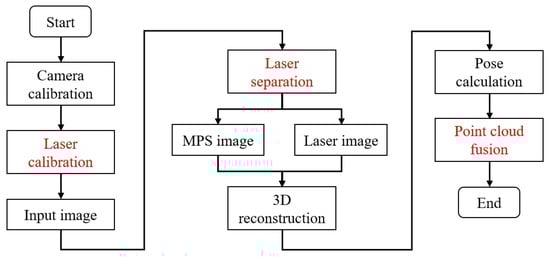
Figure 1.
Reconstruction flowchart of fusion laser triangulation and mobile multispectral photometric stereo. The steps marked in red represent our main innovations.
3.1. Calibration of Camera and Laser Plane
The calibration of a camera is mainly aimed at eliminating the impact of radial and tangential distortions of the lens on camera imaging. For nonlinear imaging models, the distortion coefficient, as an important component of camera internal parameters, can be calculated through camera calibration. This calculated distortion coefficient can be used to eliminate distortion in the original image. In this paper, we utilize the traditional camera calibration approach [20]: we first capture standard checkerboard patterns underwater at different positions and directions (shown in Figure 2), and then use the calibration toolbox provided in MATLAB to complete the camera calibration.
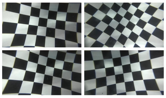
Figure 2.
Standard checkerboard for camera calibration.
After completing the calibration of the camera, its internal parameter matrix can be expressed as:
where , are focal lengths, and and are the partial derivatives of focal length f in the x and y directions. , represent principal point coordinates, and s is the coordinate axis tilt parameter, ideally 0;
Before solving the laser plane, we define the coordinate system:
- In the world coordinate system , the origin is , which can be any point in the 3D world;
- In the image coordinate system , the origin is , located in the top left corner of the image;
- In the camera coordinate system , the origin is , located in the optical center of the camera.
To solve the laser plane equation, the first step is to convert the image coordinates of the pixels on the laser line to the camera coordinate system. Due to the fact that the world coordinate system defined during camera calibration is based on the plane where the calibration plate is located as the X−O−Y plane, i.e., the plane equation of the calibration plate plane in the world coordinate system is Z = 0, the next step is to calculate the equation of the calibration plate plane in the camera coordinate system. By calibrating the camera, the rotation and translation from the world coordinate system to the camera coordinate system are obtained. R and t are transformations from the world coordinate system to the camera coordinate system, and their inverses ( and ) from the camera coordinate system to the world coordinate system are calculated as follows:
The following equation represents the correspondence between any point on the imaging plane and its coordinates in the normalized camera coordinate system:
Assuming the laser plane equation is in the camera coordinate system, the centroid positions of N 3D points on the laser plane are
We then reset the center of mass to zero:
Finally, the covariance matrix can be expressed as:
After that, we perform singular value decomposition (SVD) on the covariance matrix, and the eigenvector corresponding to the minimum eigenvalue is the normal vector of the laser plane.
We propose a sub-pixel laser line extraction method based on line fitting, whose specific workflow is as follows:
Firstly, we preprocess the obtained image by selecting the image containing laser lines and the calibration checkerboard, cropping the original image () to a resolution of that only contains the laser lines and calibration board, and positioning the laser lines in the middle of the cropped image.
Next, we perform separation and binarization of the three color channels. For the separation step, we use the image , image , and image functions in Matlab to separate the red, green, and blue component images, generating three grayscale value images, and traverse all pixels of the image for binarization; that is, the pixels of the image are either black or white, containing only two values: 0 or 1.
Then, we perform image morphology judgment, remove the influence of noise such as overexposed areas, and highlight areas based on the connected area and circularity. We mark and number the connected regions in the image, and calculate the area and perimeter of each connected region. Based on experience, we label connected regions with over 40,000 pixels as overexposed areas, which are set to 0. As for the connected regions whose area is less than 40,000 pixels, we determine their circularity using . When the circularity is greater than 0.5, the connected region is labeled as a highlight area, which is also set to 0. After that, we record the coordinates of candidate points for each channel according to the set threshold.
Finally, we fit a straight line over these candidate points and remove candidate points with low confidence based on their dispersion from the line until the optimal laser line and laser plane are obtained. More specifically, we traverse all non−zero pixels in the image, record the coordinates of each pixel, perform linear fitting, detect deviations using the rmoutliers function from Matlab, then remove these outliers. This step is repeated until the fitted line no longer changes, and the optimal laser line is obtained. The above steps are repeated to obtain the laser plane equation through multiple non−parallel optimal lines.
We provide the visualization results of these four steps and a comprehensive flowchart of our proposed algorithm in Figure 3a and Figure 3b, respectively.
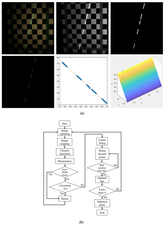
Figure 3.
(a) The first line is the captured image, green channel image and binary image, the second line is the refined image, fitted line and laser plane. (b) Workflow for obtaining the laser plane through area selection and linear fitting.
3.2. Multispectral Photometric Stereo
Ideally, only the Lambertian model can perform traditional photometric stereo reconstruction, so we assume a Lambertian reflection model without the influence of ambient light. Given three distant light sources illuminating the surface of an object, the brightness information of the surface is given by the following equation:
where c represents the brightness of the surface, and represents the albedo or the reflectivity of the surface of the object to be measured, which is a unique fixed constant for the same object. L is the direction vector of three distant light sources relative to the surface of the object being measured, which is a known quantity, and N is the normal vector of the surface. Therefore, given a set of input images, this equation can be used to reconstruct the normal direction of the object under test.
The multispectral photometric stereo (MPS) algorithm is a variation of the traditional photometric stereo algorithm, which replaces the three white lights in the traditional photometric stereo with far-point light sources of three primary colors: red, green, and blue. Multispectral photometric stereo is essentially a form of photometric stereo with three primary color (R, G, B) light sources. It replaces the time-division multiplexing (multiple single light illumination) used in traditional photometric stereo with frequency-division multiplexing (single multi-light illumination). The difference between PS and MPS is shown in Figure 4. Compared with traditional photometric stereo algorithms, the dynamic and real-time performance of single image reconstruction using multispectral photometric stereo can be used in the reconstruction of video sequences. Assuming that the object conforms to the Lambertian model, the brightness value of any point on the object in the i-th (i = 1, 2, 3, representing red, green, and blue, respectively) channel is expressed as:
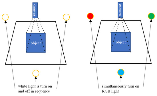
Figure 4.
Time-division multiplexing PS (left) and frequency-division multiplexing MPS (right).
In this equation, the vector V represents a combination matrix that simulates surface chromaticity, spectral distribution, camera spectral sensitivity, etc., which will be different for areas with different chromaticities. L is the direction vector of the three far-point light sources relative to the surface of the object to be measured, which is a known quantity. N is the normal vector of the surface. The decomposition of V can be expressed as:
where is the chromaticity information of the object’s surface, is the distribution information of the light source spectrum, represents the sensitivity of the camera to light, and is the albedo of the object’s surface at this point.
Multispectral photometric stereo only uses one image to calculate the surface normal direction when the overall surface chromaticity and albedo of the target object are the same. In Equation (9), and are determined by the light source and camera, which results in the image uncertainty in the mapping relationship between the grayscale values of the R, G, and B channels and the surface normal direction. In order to obtain a unique mapping value, additional restrictions need to be added. In our paper, we use the superpixel segmentation method, which divides the object’s surface into multiple areas of the same surface color and calculates a unique value of the object’s normal in each area. As this approach requires the initial depth as a prior, we add laser information to the multispectral image to provide it with a prior of the initial depth and a criterion of the true scale.
3.3. Laser Line Separation
In the process of using images with laser lines and multispectral features for 3D reconstruction, we found that some primary light sources contain the same or similar spectra as the laser lines in the image, which makes it difficult to extract laser lines through region-based image segmentation and morphological operations. In addition, the area illuminated by the laser line on the object under test will only display the color of the laser line, losing the pixel information of the corresponding color and brightness of the multispectral light source in this area. When performing direct (uncorrected) 3D reconstruction with a three-channel separation, it will cause segmentation phenomena (Figure 5), where the area marked by a red ellipse shows the unevenness of the texture or pattern caused by the reconstruction under the influence of the laser line. The mutual influence between laser and multispectral light sources greatly reduces the reconstruction performance, which puts forward another serious challenge to consider. In order to complete the reconstruction of multispectral photometric stereo, it is necessary to remove the influence of laser lines on multispectral images while retaining the laser line information.
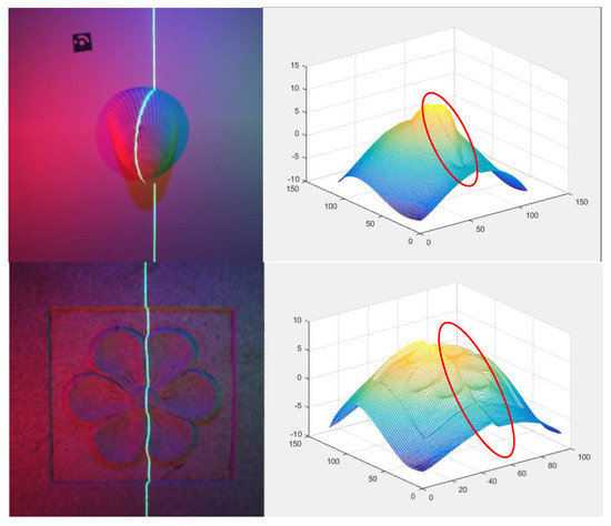
Figure 5.
Three−dimensional reconstruction of uncorrected multispectral photometric stereo, the red circle represents the reconstructed abnormal area.
We propose a method for restoring keyframe images through image sequences, and the implementation process is as follows (Figure 6):
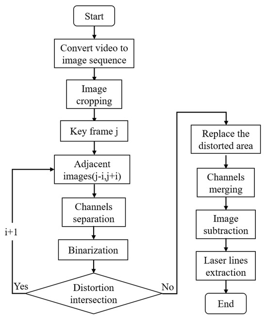
Figure 6.
Process diagram for laser line separation.
- Firstly, we select an image containing the laser line and the object to be measured, and then crop the original image according to the object’s size so that the image only contains the laser line and the object to be measured. Assuming that, in a given frame, the laser line is partially bent, then the frame is used as a keyframe to perform the three-channel separation. Threshold segmentation is performed on each channel, and their intersection is exploited to find the area where the pixel grayscale value is distorted.
- Next, we pick the adjacent image pairs (, ) of the previously selected keyframe image j. After separating these two frames into three channels, perform threshold segmentation to determine the areas where pixel grayscale values are distorted. We perform intersection processing on the distorted areas of images and to determine if there is an intersection. If there is an intersection, pick the frame and the frame to form a pair of images with larger intervals (, ). After separating the three channels, determine whether there is an intersection in the distorted area in this new pair. If there is an intersection once again, this process of searching for increasing large pairs from frame j is repeated until no intersection is found.
- Finally, the pixel values of the corresponding area (distortion area of the keyframe j) before image binarization are overlapped and evenly divided, then replaced with the distorted area of the keyframe j that has not been binarized, making it a new keyframe without a distortion area. The restored keyframe image is directly subtracted from the original keyframe image j in terms of pixel values to obtain the laser line image. The above steps are repeated until the laser line disappears from the object to be measured.
3.4. Mobile Reconstruction and Data Fusion
COLMAP is a highly integrated Structure from Motion (SfM) and Multi-View Stereo (MVS) pipeline tool that can restore the geometric structure (point cloud) of a 3D scene and the camera pose corresponding to each image from an unordered or ordered collection of 2D photos [48]. We utilize the characteristic of COLMAP to process the video sequence; we collect and record the camera pose corresponding to each keyframe during data collection. We separated the keyframes into multispectral images without laser lines and pure laser images, and combined them with the photometric stereo algorithm based on laser line correction proposed by Fan [49] for 3D reconstruction. After completing the 3D reconstruction of all keyframes, we use the camera pose to form the point cloud. Due to the continuous nature of the video sequence, although there are intervals in the selection of keyframes, the intervals between the selected key frames will inevitably lead to multiple values at the same position on the object’s surface during the reconstruction process. To address this issue, we propose a weighted data fusion method:
where is the distance between the point with multiple values and the laser line of the first image containing this point. is the distance between the point and the laser line of the second image containing this point. is the distance between the point and the laser line of the i-th image containing this point. It can be summarized as:
where D represents the final value of the point. represents the value of the point in the first image, and represents the weight of the point in the first image value. represents the value of the point in the i-th image, and represents the weight of the point in the i-th image value.
We apply a weight based on how close a point on the surface is to the location of the laser line in each image. Since the deviation in the reconstruction of the laser line position is the smallest, the closer the reconstructed data to the laser line are, the more accurate they are and the greater the weight.
4. Experiment and Comparison
4.1. Experimental Setup
In our self-made mobile equipment, the camera model is IDS UI-5240CP-C-HQ (IDS Imaging Development Systems GmbH, Obersulm, Germany), the light source model is Aozipudun AZ-SDD03-01 (Zhongshan Minfeng Lighting Co., Ltd., Zhongshan, China), and the linear laser model is Desheng DS2090 (Changshu Desheng Optoelectronics Co., Ltd., Changshu, China). We also built a pool for underwater experiments and laid sediment on the bottom of the pool to simulate the underwater environment under real conditions. The self-made equipment and experimental water tank are shown in Figure 7.
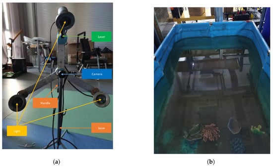
Figure 7.
(a) Self-made equipment. (b) Water tank used for experiments.
4.2. Comparison of Laser Plane Calibration Effects
The key to laser plane calibration lies in the extraction of laser lines, and the effectiveness of laser line extraction algorithms is commonly measured in terms of accuracy and efficiency. Due to the unknown true position of the laser center point, this paper proposes to measure standard blocks (the standard block is a calibration gauge block used for calibrating Vernier calipers and digital calipers). After using laser triangulation to measure standard blocks of different sizes underwater at close range, the accuracy is evaluated in terms of the mean absolute error and root mean square error between the measured height and the true height. We calculated the efficiency of different methods by extracting the time used for laser lines, and conducted efficiency experiments on an Intel (R) Core (TM) i3-7100H CPU, using a computer with a frequency of 3.90 GHz and 16 GB RAM, and using MATLAB R1016a as the software platform. The results of different methods are shown in Figure 8 and Table 1.
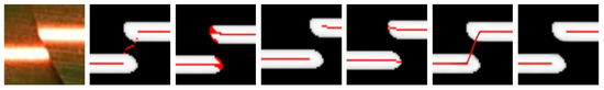
Figure 8.
Laser line detection images using different methods. From left to right are the original images, grayscale centroid [12], Steger [13], improved thinning [14], unilateral tracing [15], LBDM [16] and ours.

Table 1.
Comparison of root mean square error (RMSE) and mean absolute error (MAE) of six methods (the result unit is mm).
We compare our proposed method with two traditional methods and three newly improved methods. As can be seen from Figure 8, the grayscale centroid method still has laser scattering points outside the break point; the Steger method shows laser point clustering at the break point; the improved thinning method exhibits misalignment at one end of the break point; the unilateral tracing method presents drift at both ends of the break point; and the LBDM method displays incorrect connections in the laser line. These methods result in significant errors in laser line extraction. Our method remains unaffected at the edges and can obtain more accurate results through the relative distance between two straight lines. It can be seen from Table 1 that the MAE result of our method is at least 53% lower than the traditional grayscale centroid method, 33% lower than the Steger method, 51% lower than the improved thinning method [14], and 17% lower than the unilateral tracing method [15]. Our method is at least 2.76% lower than the LBDM method [16] in other size standard blocks, but 0.69% higher in the 30 mm standard block. The best result is displayed in bold.
In order to verify the efficiency of the algorithm, we compared the time required for each algorithm to extract laser lines from from a single image, and the results are shown in Table 2.
Table 2.
Comparison of running time of six methods.
The running time of our proposed algorithm is about 4 times faster than the grayscale centroid method, 37 times faster than the Steger method, 23 times faster than the improved thinning method, and 30 times faster than the LBDM method. Although the running time of our proposed algorithm is not the shortest, it is almost the same as the running time of the unilateral tracking method. Our method yielded a fair combination of accuracy and efficiency; the difference in running time with the unilateral tracking method is significantly small. The best result is displayed in bold.
4.3. Comparison of Laser Line Separation Effects
We selected two real objects to verify the feasibility of our proposed method. In order to obtain the ground truth for the multispectral images of the two objects in their real environment, we need to take three images separately with the device stationary. A multispectral image with the laser (input image), a multispectral image without the laser (ground truth), and a laser image (ground truth).
The results of processing images on two real objects, a shell and an airplane model, are shown in Figure 9. The lower left corner of each image is labeled. Among them, a is a multispectral image (collected image) with laser lines; b is a multispectral image without laser lines (collected image), which is also the ground truth (GT) corresponding to the multispectral image a; c is the multispectral image (predicted image) obtained by our proposed method; d is the laser line image (collected image), which is also the ground truth (GT) corresponding to the laser line we aim to obtain; e is the laser image (predicted image) obtained after taking the difference between the input image a and the output image c; and b-c is the difference map between the predicted multispectral image and its corresponding ground truth. The black area indicates no difference, and the brighter the difference, the greater the error; d-e is the difference between the predicted image of the laser line image and the ground truth. The black area means there is no difference, and the whiter the area, the greater the error.
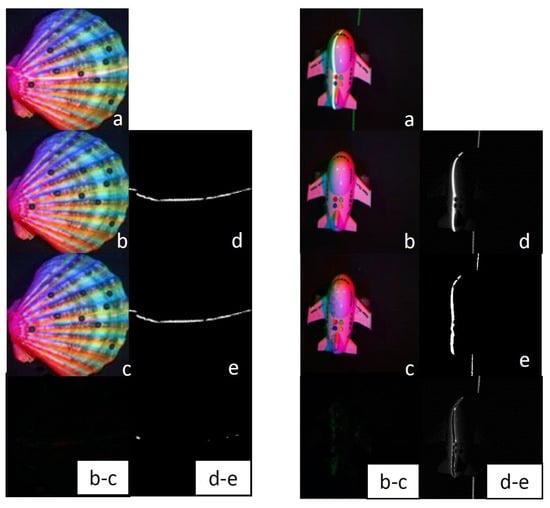
Figure 9.
The result of processing real object images. (a) is multispectral image, (b,d) are GT, (c,e) are obtained by our method.
After processing the difference between the two real objects, it can be concluded that there is almost no difference between the predicted image obtained by our method and its corresponding ground truth. Especially for the multispectral images of the shell, the processing effect of laser lines is very obvious. The difference b-c in the multispectral images is almost black everywhere, making it difficult to distinguish the position and color of the colored areas. Moreover, the difference in laser lines d-e only shows some pixel shifts. Although the estimation performance of the laser line in the multispectral image of the airplane object is not as obvious as that of the shell, the difference b-c in its multispectral image is not significant either, only a few vertical green lines appear, and the difference d-e in the laser line only exists in the outer contour of the laser line (the central area is black), indicating that the predicted laser line and its ground truth only differ in thickness, where the central area overlaps. Therefore, our proposed method is feasible and can efficiently exploit a multispectral image with laser lines to a multispectral image without laser lines and an accurate laser line.
To verify the accuracy of our method, we compared the processing results of existing commonly used algorithms with ours. The traditional algorithm for filling holes through waveform information proposed by Criminisi et al. [17] is expressed as Cr. The tensor core norm minimization algorithm proposed by Lu et al. [18] is expressed as Lu. The iterative correction algorithm of the feedback mechanism proposed by Zeng et al. [19] is expressed as Ze. The effect comparison is shown in Figure 10.
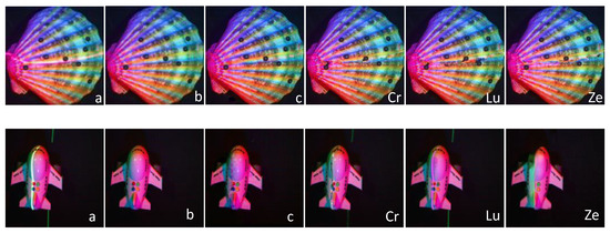
Figure 10.
Comparison of processing results of two real object images by our method and three existing methods. (a) is multispectral image, (b) is GT, and (c) is obtained by our method.
Similarly to Figure 9, the label is set in the lower right corner of the predicted image results, where a is a multispectral image with laser lines, b is a multispectral image without laser lines (GT), and c is the multispectral image predicted by our algorithm. Cr is the effect image of filling holes with redundant information, Lu is the effect image obtained by minimizing the tensor kernel norm, and Ze is the effect image of feedback iterative repair. The default image resolution is pixels.
Table 3 shows the mean absolute error (MAE) and root mean square error (RMSE) of the multispectral images restored by different methods for the shell and airplane model, compared to those of our proposed method, where the MAE results are multiplied by so that both the MAE and RMSE results are expressed with four decimal digits for better interpretation. Our method surpasses the compared methods in terms of MAE and RMSE on both the shell and airplane model, where the best prediction result is obtained on the shell. The best result is displayed in bold.
Table 3.
Comparison of three commonly used algorithms and their accuracy results with our algorithm.
4.4. Comparison of 3D Reconstruction Performance
We conducted reconstruction and verification of the carved stone slab and shell collection plate in water, and analyzed their reconstruction results.
Traditional underwater photometric stereo cannot perform mobile reconstruction, so it is impossible to reconstruct the side information of the stone slab and may result in voids, as shown in Figure 11 and Figure 12. The angle of light source illumination and the obstruction of surface undulations of objects are inherent problems in static photometric solids. The advantage of our proposed method is that it can dynamically scan and solve the problems of side reconstruction and reconstruction with holes.
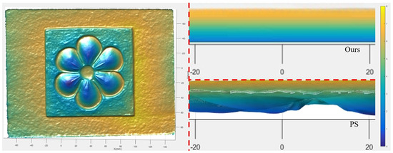
Figure 11.
Reconstruction of details on the side of carved stone slab.
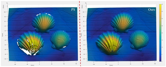
Figure 12.
Reconstruction of shell collection plate.
We conducted reconstruction verification on sea snails and shells in water, and analyzed their reconstruction results. The results obtained using the high-precision 3D reconstruction instrument (EinScan Pro, Shining 3D Tech Co., Ltd., Hangzhou, China) are represented as GT. EinScan Pro achieves high reconstruction accuracy, with a maximum resolution of up to 0.02 mm, making it suitable for precision part inspection and complex surface modeling. However, it may struggle to fully capture small holes, sharp edges, or deep groove structures, and its implementation involves relatively high costs. The reconstruction method using slow translation to simulate conveyor belt translation [50] is represented as Liu. By rotating around the camera to simulate multi-angle illumination of the event camera, multiple illumination angles will be obtained, and the reconstruction method with added laser lines [8] is represented as Yu. The method we propose is represented as Ours.
We compared the reconstruction effects of three methods including ours for shells and conches separately, and the reconstruction results are produced in PLY (Polygon) format, as shown in Figure 13. From left to right are Shell 1, Shell 2, Conch 1, Conch 2, and Conch 3. From top to bottom are GT, Liu, Yu and Ours.
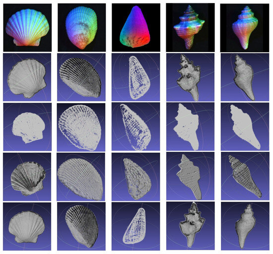
Figure 13.
Comparison of underwater shell and conch reconstruction.
From Table 4, it can be seen that our method achieved the best results on all objects. Among the shells, our methods achieved the smallest mean absolute error (MAE) of 0.29 mm on Shell 2. Our method achieved the smallest mean absolute error (MAE) of 1.72 mm. The best result is displayed in bold.
Table 4.
Comparison of mean absolute error (MAE) among methods Liu, Yu and ours.
5. Conclusions
This paper proposed a 3D reconstruction method for underwater objects that combines laser triangulation and mobile multispectral photometric stereo (MPS). This method uses a mobile MPS device to achieve dynamic reconstruction of the target object. The significance of this paper lies in the fact that our proposed method not only solves the problems of lack of scale, occlusion of shadows, and difficulty in dynamic measurement in photometric stereo in an underwater photometric stereo environment, but also the problem of sparse point clouds in an underwater laser environment. We adopted a weighted data fusion method to optimize the 3D data obtained from keyframes, and proposed an optimization method for laser plane calibration and laser line separation, further improving the reconstruction performance of laser triangulation and multispectral photometric stereo. The final experimental results indicate that our method has achieved remarkable underwater reconstruction results.
The dynamic 3D MPS reconstruction technology proposed in this paper is ultimately aimed at 3D reconstruction of objects in complex underwater environments. Specifically, based on multispectral photometric stereo, this paper utilizes a traditional laser triangulation approach to achieve high-precision 3D reconstruction of motion. Obviously, in addition to these existing hardware and methods, there will definitely be some new hardware and methods in the future to adapt to more complex reconstruction environments, such as recent inertial measurement devices and event cameras [51,52], which can further promote the development of dynamic underwater 3D reconstruction technology.
Author Contributions
Conceptualization, Y.Y. (Yang Yang) and J.D.; methodology, Y.Y. (Yang Yang) and S.Z.; software, Y.Y. (Yang Yang) and Y.L.; validation, Y.Y. (Yang Yang) and J.D.; formal analysis, Y.Y. (Yang Yang), Y.L., E.R. and Y.Y. (Yifan Yin); investigation, Y.Y. (Yang Yang); resources, J.D.; data curation, Y.Y. (Yang Yang); writing—original draft preparation, Y.Y. (Yang Yang); writing—review and editing, E.R., Y.Y. (Yifan Yin) and Y.Y. (Yang Yang); visualization, Y.Y. (Yang Yang); supervision, Y.Y. (Yang Yang), S.Z. and J.D.; project administration, J.D.; funding acquisition, S.Z. and J.D. All authors have read and agreed to the published version of the manuscript.
Funding
This research was funded by the Research and Development Plan for Major Science and Technology Innovation Projects in Shandong Province of China (2024ZLGX06), and the Natural Science Foundation of China (41927805).
Data Availability Statement
The raw data supporting the conclusions of this article will be made available by the authors on request.
Conflicts of Interest
The authors declare no conflicts of interest.
References
- Rajapan, D.; Rajeshwari, P.M.; Zacharia, S. Importance of Underwater Acoustic Imaging Technologies for Oceanographic applications—A brief review. In Proceedings of the OCEANS 2022, Chennai, India, 21–24 February 2022; pp. 1–6. [Google Scholar]
- Shen, Y.; Zhao, C.; Liu, Y.; Wang, S.; Huang, F. Underwater Optical Imaging: Key Technologies and Applications Review. IEEE Access 2021, 9, 85500–85514. [Google Scholar] [CrossRef]
- Hu, K.; Wang, T.; Shen, C.; Weng, C.; Zhou, F.; Xia, M.; Weng, L. Overview of underwater 3D reconstruction technology based on optical images. J. Mar. Sci. Eng. 2023, 11, 949. [Google Scholar] [CrossRef]
- Csencsics, E.; Schlarp, J.; Glaser, T.; Wolf, T.; Schitter, G. Reducing the Speckle-Induced Measurement Uncertainty in Laser Triangulation Sensors. IEEE Trans. Instrum. Meas. 2023, 72, 7000809. [Google Scholar] [CrossRef]
- Wang, X.; Jian, Z.; Yuan, H.; Ren, M. Self-Calibrating Sparse Far-Field Photometric Stereo With Collocated Light. IEEE Trans. Instrum. Meas. 2022, 71, 5001310. [Google Scholar] [CrossRef]
- Yang, Y.; Rigall, E.; Fan, H.; Dong, J. Point Light Measurement and Calibration for Photometric Stereo. IEEE Trans. Instrum. Meas. 2024, 73, 5001011. [Google Scholar] [CrossRef]
- Chakrabarti, A.; Sunkavalli, K. Single-image RGB Photometric Stereo With Spatially-varying Albedo. In Proceedings of the IEEE Fourth International Conference on 3D Vision (3DV), Stanford, CA, USA, 25–28 October 2016. [Google Scholar]
- Yu, B.; Ren, J.; Han, J.; Wang, F.; Liang, J.; Shi, B. EventPS: Real-Time Photometric Stereo Using an Event Camera. In Proceedings of the IEEE/CVF Conference on Computer Vision and Pattern Recognition (CVPR), Seattle, WA, USA, 16–22 June 2024; pp. 9602–9611. [Google Scholar]
- Fan, J.; Jing, F.; Fang, Z.; Liang, Z. A simple calibration method of structured light plane parameters for welding robots. In Proceedings of the 35th Chinese Control Conference (CCC), Chengdu, China, 27–29 July 2016. [Google Scholar]
- Xie, Z.; Wang, X.; Chi, S. Simultaneous calibration of the intrinsic and extrinsic parameters of structured-light sensors. Opt. Lasers Eng. 2014, 58, 9–18. [Google Scholar] [CrossRef]
- Zou, X.; He, H.; Wu, Y.; Chen, Y.; Xu, M. Automatic 3D point cloud registration algorithm based on triangle similarity ratio consistency. IET Image Process. 2020, 14, 3314–3323. [Google Scholar] [CrossRef]
- Dong, M.; Xu, L.; Wang, J.; Sun, P.; Zhu, L. Variable-weighted grayscale centroiding and accuracy evaluating. Adv. Mech. Eng. 2013, 5, 428608. [Google Scholar] [CrossRef]
- Qi, L.; Zhang, Y.; Zhang, X.; Wang, S.; Xie, F. Statistical behavior analysis and precision optimization for the laser stripe center detector based on Steger’s algorithm. Opt. Express 2013, 21, 13442–13449. [Google Scholar] [CrossRef]
- Zhou, X.; Wang, H.; Li, L.; Zheng, S.; Fu, J.; Tian, Q. Line laser center extraction method based on the improved thinning method. Electron. Meas. Technol. 2023, 46, 84–89. [Google Scholar]
- Huang, Y.; Kang, W.; Lu, Z. Improved Structured Light Centerline Extraction Algorithm Based on Unilateral Tracing. Photonics 2024, 11, 723. [Google Scholar] [CrossRef]
- Zhao, X.; Yu, D.; Shi, H. Laser Stripe Extraction for 3D Reconstruction of Complex Internal Surfaces. IEEE Access 2025, 13, 5562–5574. [Google Scholar] [CrossRef]
- Criminisi, A.; Pérez, P.; Toyama, K. Region filling and object removal by exemplar-based image inpainting. IEEE Trans. Image Process. 2004, 13, 1200–1212. [Google Scholar] [CrossRef] [PubMed]
- Lu, C.; Feng, J.; Lin, Z.; Yan, S. Exact low tubal rank tensor recovery from Gaussian measurements. arXiv 2018, arXiv:1806.02511. [Google Scholar]
- Zeng, Y.; Lin, Z.; Yang, J.; Zhang, J.; Shechtman, E.; Lu, H. High-resolution image inpainting with iterative confidence feedback and guided upsampling. In Proceedings of the Computer Vision—ECCV 2020: 16th European Conference, Glasgow, UK, 23–28 August 2020; Proceedings, Part XIX 16. pp. 1–17. [Google Scholar]
- Zhang, Z. A Flexible New Technique for Camera Calibration. IEEE Trans. Pattern Anal. Mach. Intell. 2000, 22, 1330–1334. [Google Scholar] [CrossRef]
- Hong, Y.; Ren, G.; Liu, E. Non-iterative method for camera calibration. Opt. Express 2015, 23, 23992–24003. [Google Scholar] [CrossRef]
- Niu, Z.; Zhang, Z.; Wang, Y.; Liu, K.; Deng, X. Calibration method for the relative orientation between the rotation axis and a camera using constrained global optimization. Meas. Sci. Technol. 2017, 28, 055001. [Google Scholar] [CrossRef]
- Zheng, F.; Kong, B. Calibration of linear structured light system by planar checkerboard. In Proceedings of the IEEE International Conference on Information Acquisition, Hefei, China, 21–25 June 2004. [Google Scholar]
- Chu, C.W.; Hwang, S.; Jung, S.K. Calibration-free approach to 3D reconstruction using light stripe projections on a cube frame. In Proceedings of the Third International Conference on 3-D Digital Imaging and Modeling, Quebec City, QC, Canda, 28 May–1 June 2001. [Google Scholar]
- Chi, S.; Xie, Z.; Chen, W. A Laser Line Auto-Scanning System for Underwater 3D Reconstruction. Sensors 2016, 16, 1534. [Google Scholar] [CrossRef]
- Lin, H.; Zhang, H.; Li, Y.; Huo, J.; Deng, H.; Zhang, H. Method of 3D reconstruction of underwater concrete by laser line scanning. Opt. Lasers Eng. 2024, 183, 108468. [Google Scholar] [CrossRef]
- Jiang, S.; Sun, F.; Gu, Z.; Zheng, H.; Nan, W.; Yu, Z. Underwater 3D reconstruction based on laser line scanning. In Proceedings of the OCEANS 2017, Aberdeen, UK, 19–22 June 2017; pp. 1–6. [Google Scholar]
- Li, J.; Zhou, Q.; Li, X.; Chen, R.; Ni, K. An Improved Low-Noise Processing Methodology Combined with PCL for Industry Inspection Based on Laser Line Scanner. Sensors 2019, 19, 3398. [Google Scholar] [CrossRef]
- Feng, Y.; Tang, J.; Su, B.; Su, Q.; Zhou, Z. Point Cloud Registration Algorithm Based on the Grey Wolf Optimizer. IEEE Access 2020, 8, 143375–143382. [Google Scholar] [CrossRef]
- Liang, L.; Ming, Y.; Chunxiang, W.; Bing, W. Robust Point Set Registration Using Signature Quadratic Form Distance. IEEE Trans. Cybern. 2018, 50, 2097–2109. [Google Scholar]
- Zhao, H. High-Precision 3D Reconstruction for Small-to-Medium-Sized Objects Utilizing Line-Structured Light Scanning: A Review. Remote. Sens. 2021, 13, 4457. [Google Scholar]
- Hua, L.; Lu, Y.; Deng, J.; Shi, Z.; Shen, D. 3D reconstruction of concrete defects using optical laser triangulation and modified spacetime analysis. Autom. Constr. 2022, 142, 104469. [Google Scholar] [CrossRef]
- Liu, L.; Cai, H.; Tian, M.; Liu, D.; Cheng, Y.; Yin, W. Research on 3D reconstruction technology based on laser measurement. J. Braz. Soc. Mech. Sci. Eng. 2023, 45, 297. [Google Scholar] [CrossRef]
- Huang, H.; Liu, G.; Xiao, C.; Deng, L.; Gong, Y.; Song, T.; Qin, F. Spatial quadric calibration method for multi-line laser based on diffractive optical element. AIP Adv. 2024, 14, 035017. [Google Scholar] [CrossRef]
- Hong, H.; Lee, B.H. Probabilistic normal distributions transform representation for accurate 3D point cloud registration. In Proceedings of the 2017 IEEE/RSJ international Conference on intelligent robots and systems (IROS), Vancouver, BC, Canada, 24–28 September 2017; pp. 3333–3338. [Google Scholar]
- Yuan, Y.; Wu, Y.; Lei, J.; Hu, C.; Gong, M.; Fan, X.; Ma, W.; Miao, Q. Learning compact transformation based on dual quaternion for point cloud registration. IEEE Trans. Instrum. Meas. 2024, 73, 2506312. [Google Scholar] [CrossRef]
- Zhao, F.; Huang, H.; Hu, W. An optimized hierarchical point cloud registration algorithm. Multimed. Syst. 2025, 31, 14. [Google Scholar] [CrossRef]
- Narasimhan, S.; Nayar, S. Structured light methods for underwater imaging: Light stripe scanning and photometric stereo. In Proceedings of the OCEANS 2005, Washington, DC, USA, 18–23 September 2005; pp. 2610–2617. [Google Scholar]
- Tsiotsios, C.; Angelopoulou, M.E.; Kim, T.K.; Davison, A.J. Backscatter Compensated Photometric Stereo with 3 Sources. In Proceedings of the IEEE/CVF Conference on Computer Vision and Pattern Recognition (CVPR), Columbus, OH, USA, 24–27 June 2014. [Google Scholar]
- Jiao, H.; Luo, Y.; Wang, N.; Qi, L.; Lei, H. Underwater multi-spectral photometric stereo reconstruction from a single RGBD image. In Proceedings of the 2016 Asia-Pacific Signal and Information Processing Association Annual Summit and Conference (APSIPA), Jeju, Republic of Korea, 13–16 December 2017. [Google Scholar]
- Fan, H.; Qi, L.; Chen, C.; Rao, Y.; Kong, L.; Dong, J.; Yu, H. Underwater Optical 3-D Reconstruction of Photometric Stereo Considering Light Refraction and Attenuation. IEEE J. Ocean. Eng. 2022, 47, 46–58. [Google Scholar] [CrossRef]
- Zhou, M.; Ding, Y.; Ji, Y.; Young, S.S.; Ye, J. Shape and Reflectance Reconstruction Using Concentric Multi-Spectral Light Field. IEEE Trans. Pattern Anal. Mach. Intell. 2020, 42, 1594–1605. [Google Scholar] [CrossRef]
- Yakun, J.; Lin, Q.; Huiyu, Z.; Junyu, D.; Liang, L. Demultiplexing Colored Images for Multispectral Photometric Stereo via Deep Neural Networks. IEEE Access 2018, 6, 30804–30818. [Google Scholar]
- Hamaen, K.; Miyazaki, D.; Hiura, S. Multispectral Photometric Stereo Using Intrinsic Image Decomposition. In Proceedings of the IW-FCV 2020, Tokyo, Japan, 20–22 February 2020. [Google Scholar]
- Guo, H.; Okura, F.; Shi, B.; Funatomi, T.; Mukaigawa, Y.; Matsushita, Y. Multispectral Photometric Stereo for Spatially-Varying Spectral Reflectances. Int. J. Comput. Vis. 2022, 130, 2166–2183. [Google Scholar] [CrossRef]
- Miyazaki, D.; Uegomori, K. Example-Based Multispectral Photometric Stereo for Multi-Colored Surfaces. J. Imaging 2022, 8, 107. [Google Scholar] [CrossRef] [PubMed]
- Lu, L.; Zhu, H.; Dong, J.; Ju, Y.; Zhou, H. Three-Dimensional Reconstruction with a Laser Line Based on Image In-Painting and Multi-Spectral Photometric Stereo. Sensors 2021, 21, 2131. [Google Scholar] [CrossRef]
- Pan, L.; Baráth, D.; Pollefeys, M.; Schönberger, J.L. Global structure-from-motion revisited. In Proceedings of the European Conference on Computer Vision (ECCV), Milan, Italy, 29 September–4 October 2024; pp. 58–77. [Google Scholar]
- Fan, H.; Rao, Y.; Rigall, E.; Qi, L.; Wang, Z.; Dong, J. Near-field photometric stereo using a ring-light imaging device. Signal Process. Image Commun. 2022, 102, 116605. [Google Scholar] [CrossRef]
- Liu, H.; Wu, X.; Yan, N.; Yuan, S.; Zhang, X. A novel image registration-based dynamic photometric stereo method for online defect detection in aluminum alloy castings. Digit. Signal Process. 2023, 141, 104165. [Google Scholar] [CrossRef]
- Niu, J.; Zhong, S.; Zhou, Y. IMU-Aided Event-based Stereo Visual Odometry. In Proceedings of the 2024 IEEE International Conference on Robotics and Automation (ICRA), Yokohama, Japan, 19–23 May 2024. [Google Scholar]
- Cho, H.; Kang, J.Y.; Yoon, K.J. Temporal Event Stereo via Joint Learning with Stereoscopic Flow. In Proceedings of the European Conference on Computer Vision (ECCV), Paris, France, 26–27 March 2025. [Google Scholar]
Disclaimer/Publisher’s Note: The statements, opinions and data contained in all publications are solely those of the individual author(s) and contributor(s) and not of MDPI and/or the editor(s). MDPI and/or the editor(s) disclaim responsibility for any injury to people or property resulting from any ideas, methods, instructions or products referred to in the content. |
© 2025 by the authors. Licensee MDPI, Basel, Switzerland. This article is an open access article distributed under the terms and conditions of the Creative Commons Attribution (CC BY) license (https://creativecommons.org/licenses/by/4.0/).