Article

Research on Sea Ice and Local Ice Load Monitoring System for Polar Cargo Vessels

1
School of Ocean and Civil Engineering, Shanghai Jiao Tong University, Shanghai 200240, China
2
State Key Laboratory of Maritime Technology and Safety, Shanghai Ship and Shipping Research Institute Co., Ltd., Shanghai 200135, China
3
Key Laboratory of Marine Technology Ministry of Communications, Shanghai Ship and Shipping Research Institute Co., Ltd., Shanghai 200135, China
4
State Key Laboratory of Industrial Equipment Structure Analysis and Optimization and CAE Software, Dalian University of Technology, Dalian 116024, China
*
Author to whom correspondence should be addressed.
J. Mar. Sci. Eng. 2025, 13(4), 808; https://doi.org/10.3390/jmse13040808
Submission received: 13 March 2025 / Revised: 11 April 2025 / Accepted: 14 April 2025 / Published: 18 April 2025

Abstract

:
Sea ice and the resulting loads are major safety concerns for vessels operating in ice-covered regions. This study presents a tailored sea ice and local ice load monitoring system specifically designed for polar cargo vessels. The system employs shipboard cameras coupled with a DeepLab v3+-based algorithm to achieve real-time ice concentration identification, demonstrating 90.68% accuracy when validated against historical Arctic Sea ice imagery. For structural load monitoring, we developed a hybrid methodology integrating numerical simulations, full-scale strain measurements, and classification society standards, enabling the precise evaluation of ice-induced structural responses. The system’s operational process is demonstrated through comprehensive case studies of characteristic ice collision scenarios. Furthermore, this system serves as an exemplary implementation of a navigation assistance framework for polar cargo vessels, offering both real-time operational guidance and long-term reference data for enhancing ice navigation safety.

1. Introduction

The development of the Arctic shipping routes has revolutionized global maritime transportation, offering substantial advantages for ports situated north of 30° N latitude on both sides of the Pacific Ocean. Vessels utilizing these polar routes can achieve voyage time reductions exceeding 40% compared to traditional routes via the Suez or Panama Canals [1,2]. A significant milestone occurred in 2013 when the M/V Yongsheng completed China’s first commercial transit through the Northeast Passage [3], marking the beginning of accelerated Chinese commercial activities in Arctic waters. By 2024, this initiative had expanded to over 60 successful transits, significantly advancing China’s Ice Silk Road development strategy. Nevertheless, the majority of commercial vessels operating in these waters either carry low ice-class certifications or lack proper ice-strengthening altogether [4]. This technical limitation substantially compromises their ice collision resistance [5], creating elevated operational risks in ice-covered zones. The safety implications of this situation warrant particular attention, as current vessel specifications may be inadequate for the challenging Arctic environment.
Structural health monitoring (SHM) systems have emerged as a critical technology for ensuring maritime safety, with particular relevance to Arctic navigation [6]. Since its initial conceptualization in 1978, SHM technology has undergone four decades of continuous development, maturing into comprehensive real-time monitoring solutions for open-water conditions. The commercial market now offers robust hardware–software integrated systems capable of monitoring multiple shipboard parameters, including structural stress distribution [7], hull vibration [8], six-degree-of-freedom motion response [9], and shafting system performance [10]. The unique working environment in the ice region puts forward a new demand for structural health monitoring.
Polar maritime operations face multifaceted hazards arising from both environmental and operational factors, including sea ice, wind, waves, ocean currents, heavy fog, and extreme temperatures, as well as the potential for human error and technical malfunctions aboard ships [11]. Among these, sea ice constitutes the most critical hazard in Arctic and Antarctic waters, necessitating the precise identification and evaluation of ice conditions to ensure navigational safety [12,13]. Recent advances in digital image processing technologies have progressively supplanted conventional manual approaches, enabling more precise differentiation of various sea ice types and the reliable extraction of critical sea ice parameters [14]. The unique visual properties of sea ice have historically led to the predominant use of binarization techniques in conventional ice detection methodologies for delineating sea ice boundaries [15]. Traditional binarization approaches, whether employing global or adaptive thresholding techniques, demonstrate significant limitations in sea ice analysis [16]. Recent advances in machine learning have demonstrated remarkable capabilities in addressing complex image semantic segmentation tasks, particularly in challenging environmental monitoring applications [17]. Notably, support vector machine (SVM) algorithms have demonstrated particular efficacy in sea ice analysis, achieving two critical breakthroughs in polar research: the accurate classification of sea ice types in both satellite remote sensing imagery and shipborne visual data [18,19] and the quantitative estimation of deformed ice thickness through feature extraction from flipped ice blocks [20].
Ice loads present a significant hazard for ships operating in ice-covered regions. Ice loads can be categorized as global ice loads and local ice loads, which respectively relate to navigation resistance and local impact [21]. Excessive ice loads can result in ice entrapment and structural damage. Arctic countries have made significant advancements in monitoring methods [22], identification methods [23], and data analysis for ice loads due to their favorable geographical position [24]. The operation of cargo vessels in polar regions presents unique structural challenges that necessitate specialized engineering solutions. Modern polar-class cargo ships incorporate substantial hull reinforcements. Despite these design enhancements, navigation through high-concentration ice fields generally requires icebreaker escort. Therefore, the main concern is navigating through broken ice and ensuring structural safety in the face of local ice loads. Researchers from Finland, Norway, and the United States have developed local ice load monitoring and alarm systems to enhance the safety of polar cargo vessels in icy conditions [25,26]. The monitoring systems employ real-time comparison between measured ice loads and design thresholds, incorporating predefined criteria to trigger appropriate warnings. It is important to note that structural safety evaluation requires more than just ice load monitoring; it must consider the permissible stress limits of critical structural elements to achieve a complete assessment.
This paper outlines a sea ice and ice load monitoring system implemented for polar cargo vessels, with the primary goal of ensuring the safe navigation of ships in ice-covered zones. Section 2 introduces a sea ice monitoring system utilizing shipborne cameras and proposes a deep learning model based on the DeepLab v3+ framework for accurately identifying sea ice concentration. The system provides detailed sea ice concentration identification results for two separate voyages, using a dataset compiled from historical sea ice images from previous expeditions. Section 3 presents an innovative ice load monitoring system that integrates numerical simulation, full-scale measurement, and standardized computational methods to address the dual challenges of ice load quantification and structural assessment for ships navigating in ice-covered waters.

2. Sea Ice Monitoring

Shipborne sea ice image monitoring serves as the most effective method for obtaining accurate measurements of critical ice parameters, including concentration, floe size, and thickness. This approach provides highly localized data with operational flexibility, offering valuable ground-truth validation that enhances the broader perspective of satellite-based remote sensing systems. The direct observation capability enables precise documentation of ice characteristics at the vessel scale while maintaining adaptability to regional ice condition variations [27].

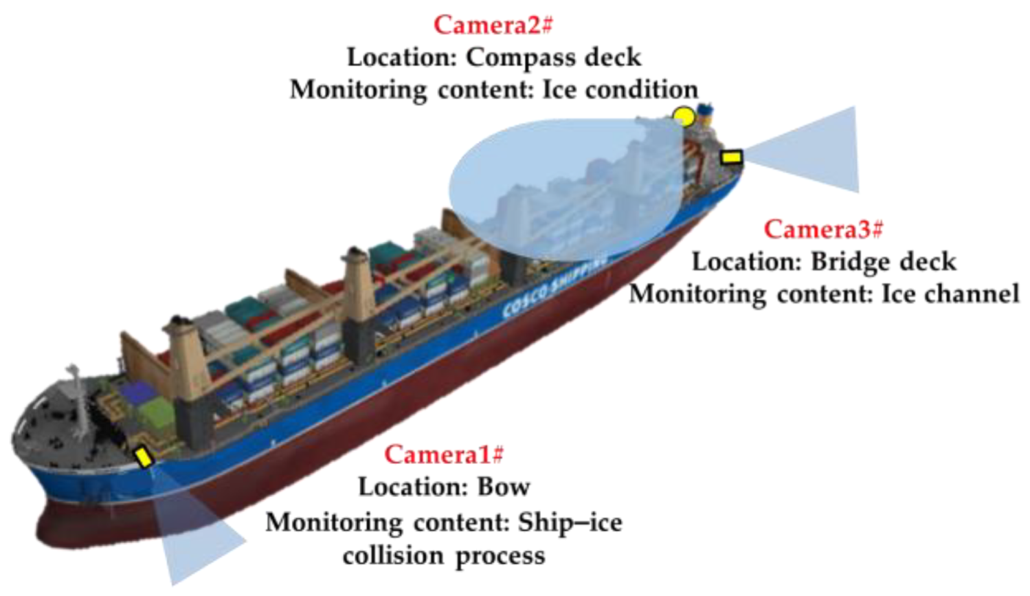
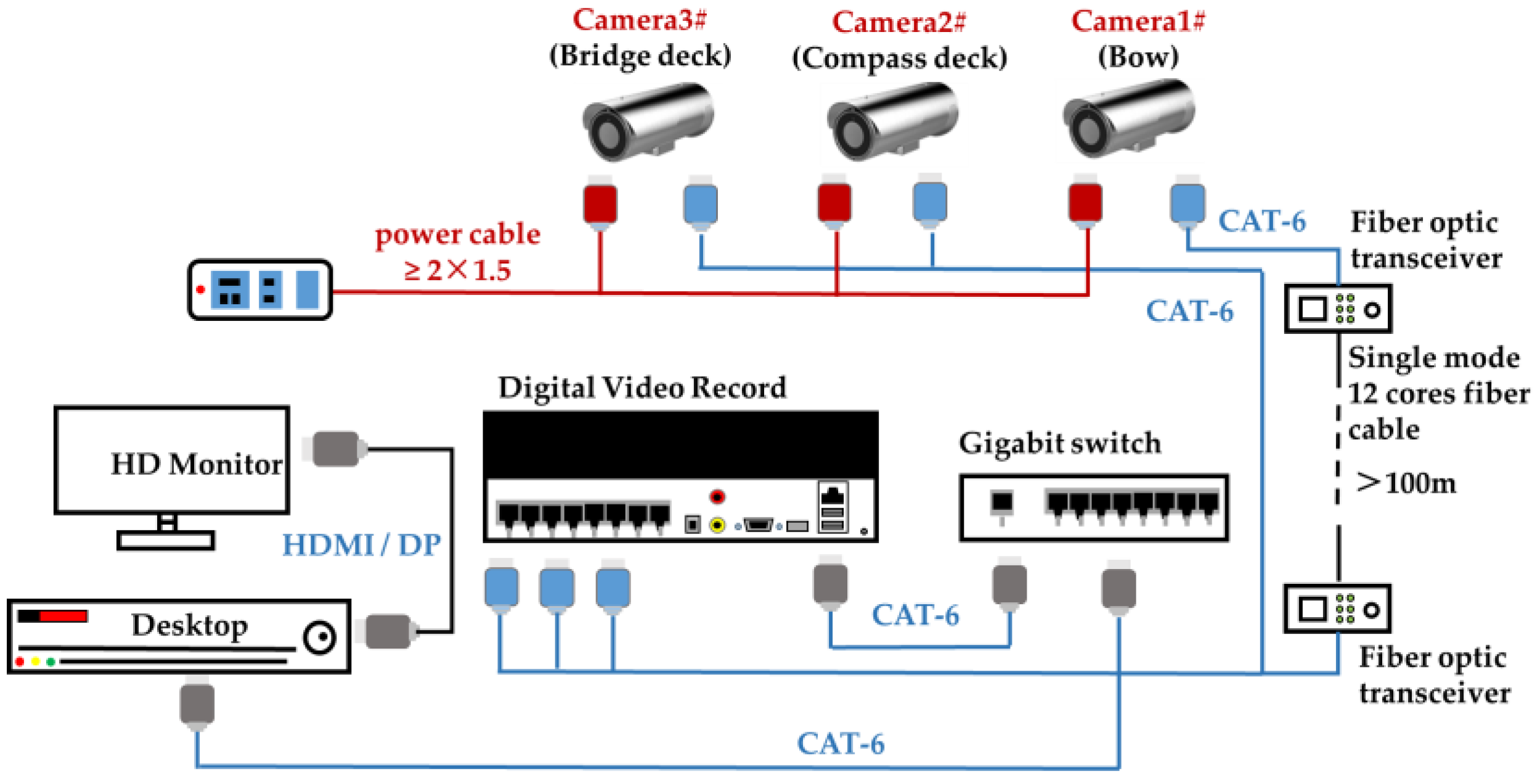
2.1. Camera-Based Sea Ice Image Monitoring

The strategic deployment of multiple cameras aboard the 68,000-ton polar multi-purpose vessel enables comprehensive acquisition of sea ice data from complementary perspectives, as illustrated in Figure 1. The selected camera positions were optimized for unobstructed fields of view and operational criticality. The bow-mounted camera provides irreplaceable observational value due to its proximity to the ship–ice interaction zone, while the port bow-mounted camera captures critical collision dynamics, icebreaking patterns, and thickness measurements. The compass deck (the superstructure’s highest point) offers an elevated vantage point that maximizes the monitoring range and minimizes blind spots from deck equipment; a compass deck camera further enhances forward-looking assessments of the ice concentration and spatial distribution. The bridge deck camera serves dual purposes: monitoring post-breakup ice channel morphology during transit and ensuring safe convoy following distances via continuous surveillance. Although relocatable in theory, the aft-facing bridge deck camera’s current position avoids exhaust stack interference while maintaining installation feasibility. This integrated configuration enables systematic documentation of ice conditions across all navigation phases.
The connection diagram of the sea ice image monitoring device is illustrated in Figure 2. The monitoring system comprises a power supply, video capture (cameras), video transmission equipment, digital video storage (DVR), and high-definition (HD) monitor. It is noteworthy that the maximum effective transmission distance for Category 6 (CAT-6) Ethernet cables is standardized at 100 m to guarantee signal fidelity and bandwidth preservation. Beyond this threshold, signal degradation necessitates the use of network extension devices. In the current full-scale implementation, the required cabling span from the bow to the bridge exceeds 200 m. To overcome this constraint while maintaining data integrity, single-mode fiber optic cabling was implemented for the bow camera, leveraging its capability for reliable data transmission over distances extending to tens of kilometers without signal attenuation concerns.

2.2. Sea Ice Concentration Identification

2.2.1. Semantic Segmentation Model of Sea Ice

This study employs the DeepLab V3+ architecture, a seminal encoder–decoder model for semantic segmentation, with critical modifications to address the computational constraints of maritime deployment environments [28]. Recognizing the hardware limitations typical of shipborne systems, we replace the conventional Xception backbone with the more efficient MobileNetv2, which leverages 1 × 1 convolutions and 3 × 3 depthwise separable convolutions to achieve significant reductions in computational complexity while maintaining feature extraction capability. The implementation utilizes an NVIDIA V100 GPU (PCIe 32 GB) within a TensorFlow 2.4 framework (Python 3.8, CUDA 11.2), employing momentum gradient descent optimization (μ = 0.9) with a polynomial learning rate decay strategy (initial α = 7 × 10⁻³) across 10,000 training iterations. This optimized configuration achieves a balance between computational efficiency and segmentation accuracy, as detailed in the architectural schematic presented in Figure 3.
The dataset consists of sea ice imagery collected during commercial transits through the Arctic’s Northeast Passage, featuring operational data from the M/V Tianyou (2018) and M/V Tianen (2019), with their respective routes illustrated in Figure 4a. Ship-mounted cameras systematically captured both forward-looking and broadside ice conditions (Figure 4b), though the analysis predominantly utilizes side-view imagery to mitigate potential visual obstructions from vessel superstructures. Comprising 500 carefully selected images, the dataset was partitioned into 400 training samples and 100 test samples to ensure robust model evaluation, with all images representing authentic navigation conditions encountered during Arctic operations.

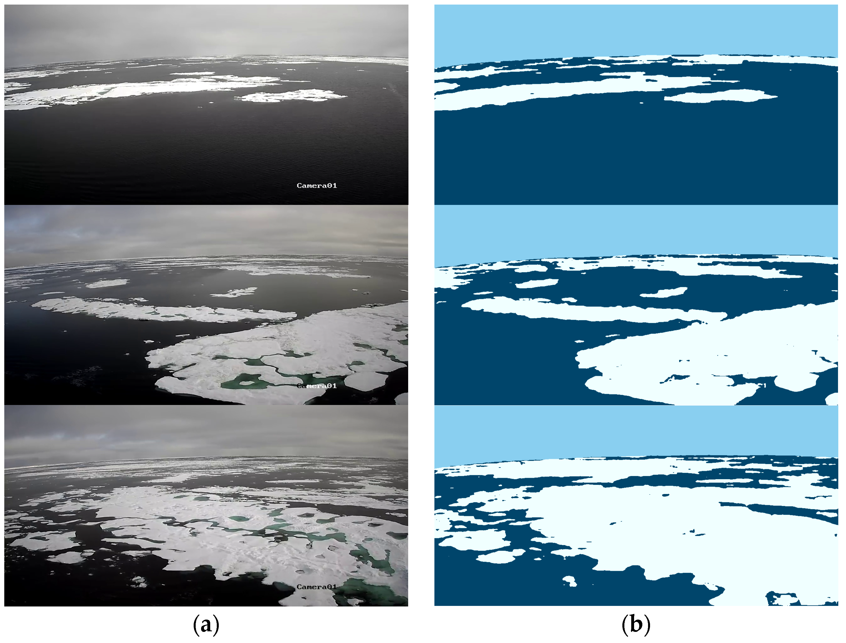
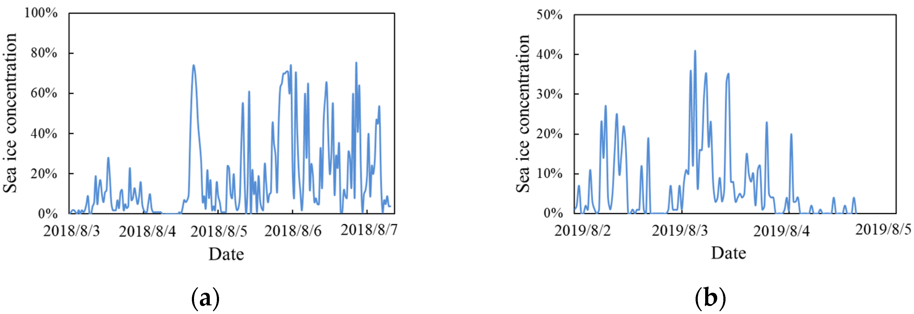
2.2.2. Results and Analysis of Sea Ice Concentration Identification

The network was trained using the aforementioned model, with sea ice images from the validation set employed as inputs to assess the classification performance of the sea ice identification model. Figure 5 presents the image recognition results for typical sea ice scenarios, demonstrating exceptional identification accuracy for sea ice, seawater and sky.
The sea ice concentration is defined as the ratio of sea ice area to the total sea area. In the context of image analysis, this is represented by the proportion of sea ice pixels relative to the combined count of sea ice and open-water pixels. For semantic segmentation tasks, the Intersection over Union (IoU) serves as the primary evaluation metric. The IoU quantifies the overlap between predicted and ground-truth segmentation masks for each class by computing the ratio of their intersection to their union. The mean IoU (mIoU), an aggregate measure of segmentation accuracy, is derived by averaging the IoU values across all classes. The corresponding mathematical expressions are as follows:
I o U = i n i i t i + j n j i n i i
m I o U = 1 n i n i i t i + j n j i n i i
where n is the number of categories; n i i is the number of pixels correctly predicted as class i , t i is the total number of pixels of class i in the label, and n j i is the total number of pixels predicted as class i .
The IoU metric measures how closely a predicted category aligns with its ground truth, whereas mIoU reflects the model’s overall segmentation accuracy. The validation set’s identification performance is summarized in Table 1, showing that the sea ice recognition accuracy achieved 90%, which satisfies the practical requirements for ship navigation applications. Furthermore, we analyzed the ice concentration identification results along shipping routes during 2018–2019. Figure 6 displays the corresponding time series of ice concentration variations. Since commercial vessels typically avoid areas with extensive ice, the observed ice concentrations were primarily classified as very open drift ice and open drift ice.
Short-term variations in the sea ice concentration offer crucial navigation guidance by revealing immediate ice conditions. As shown in Figure 6a, the route experienced a dramatic 80% maximum concentration fluctuation on 5 August. Following the M/V Tianyou’s entry into the ice zone on 3 August, concentrations persistently maintained high levels, consistently exceeding 50% from 5–8 August. These observations demonstrate substantial sea ice variability along Arctic shipping routes, necessitating speed adjustments when encountering high-concentration areas to reduce collision risks and ensure safe navigation. Additionally, ship-based image measurements of the sea ice concentration provide important complementary data to satellite remote sensing, helping overcome some spatial resolution limitations inherent in large-scale ice monitoring systems.

3. Local Ice Load Monitoring

The primary research challenges in local ice load on hull structures reside in both the accurate acquisition of ice load data and the comprehensive assessment of its structural impact.

3.1. Methodology

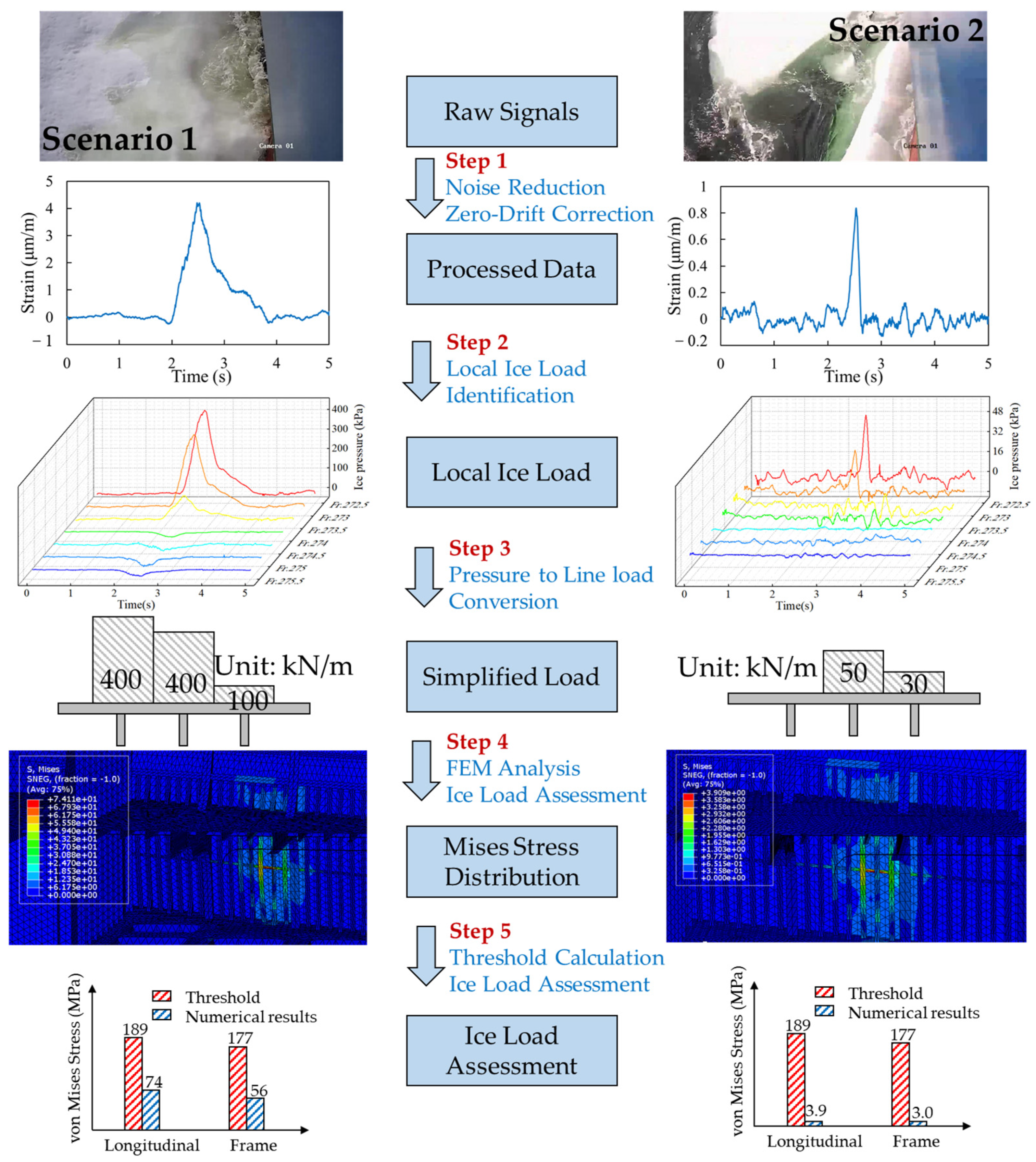
3.1.1. The Research Framework for Ice Load Acquisition and Assessment

The conceptual framework for ice load monitoring and early warning systems was first introduced in 2002, comprising four integrated subsystems: structural response measurement instrumentation, sensor data acquisition and telemetry systems, computational processing algorithms, and visualization interfaces [29,30].
This study establishes a comprehensive research framework, as shown in Figure 7, to address two critical challenges in ice load monitoring: ice load acquisition and assessment. For the target vessel, numerical simulations incorporating ship-type characteristics, structural configurations, and ice navigation peculiarities are conducted to obtain global ice pressure distributions, enabling the development of customized monitoring schemes focused on primary ice-impact zones. Full-scale measurements of shear strain in key load-bearing members—frames—are processed through advanced data interpretation techniques to indirectly determine local ice loads. These experimentally derived ice loads are subsequently applied to the local finite element model to compute equivalent stress distributions within the structural components. Critical nodal points exhibiting stress concentrations are identified for failure risk assessment, with evaluation thresholds determined by reference formulas specified in relevant classification standards. The integrated methodology combines numerical simulation, experimental measurement, and computational analysis to provide a robust solution for ice load characterization and structural safety assessment.

3.1.2. The Design of the Ice Load Monitoring Scheme

The bow region represents the most critical zone for ice–structure interaction, being both the primary contact area and most frequently impacted portion of the hull. For polar multi-purpose vessels, the significant vertical separation between upper and lower ice waterlines (UIWLs and LIWLs) makes comprehensive instrumentation of the entire forward ice belt region prohibitively expensive. Furthermore, conventional monitoring approaches relying on the empirical selection of measurement zones frequently result in spatial discrepancies between instrumented areas and actual ice-impact regions. To address this challenge, numerical simulations using discrete element methods (specifically the SDEM 2.0 software [31]) were employed to characterize ice pressure distributions under typical operational conditions, with particular emphasis on loading patterns within the ice zone.
Taking a CCS Ice Class B1 polar merchant vessel as a case study, Figure 8 presents both the spatial pressure distribution and temporal load history obtained through numerical simulation, which collectively inform the optimal sensor placement strategy for identifying critical stress concentration zones. This reveals maximum loading at the stem during straight-line ice transit—a consequence of the distinctive bow geometry differentiating polar multi-purpose vessels from dedicated icebreakers. While this finding suggests stem-proximate monitoring as ideal, practical constraints, including dense structural congestion and spatial limitations, necessitated sensor placement on frames between Fr. 272.5 and Fr. 275.5, selected through careful analysis of bow structural plans to balance measurement fidelity with installation feasibility.
The local ice load monitoring system employs a biaxial strain rosette configuration, comprising two orthogonally positioned uniaxial strain sensors for simultaneous shear strain measurement at targeted locations [32], as shown in Figure 9.

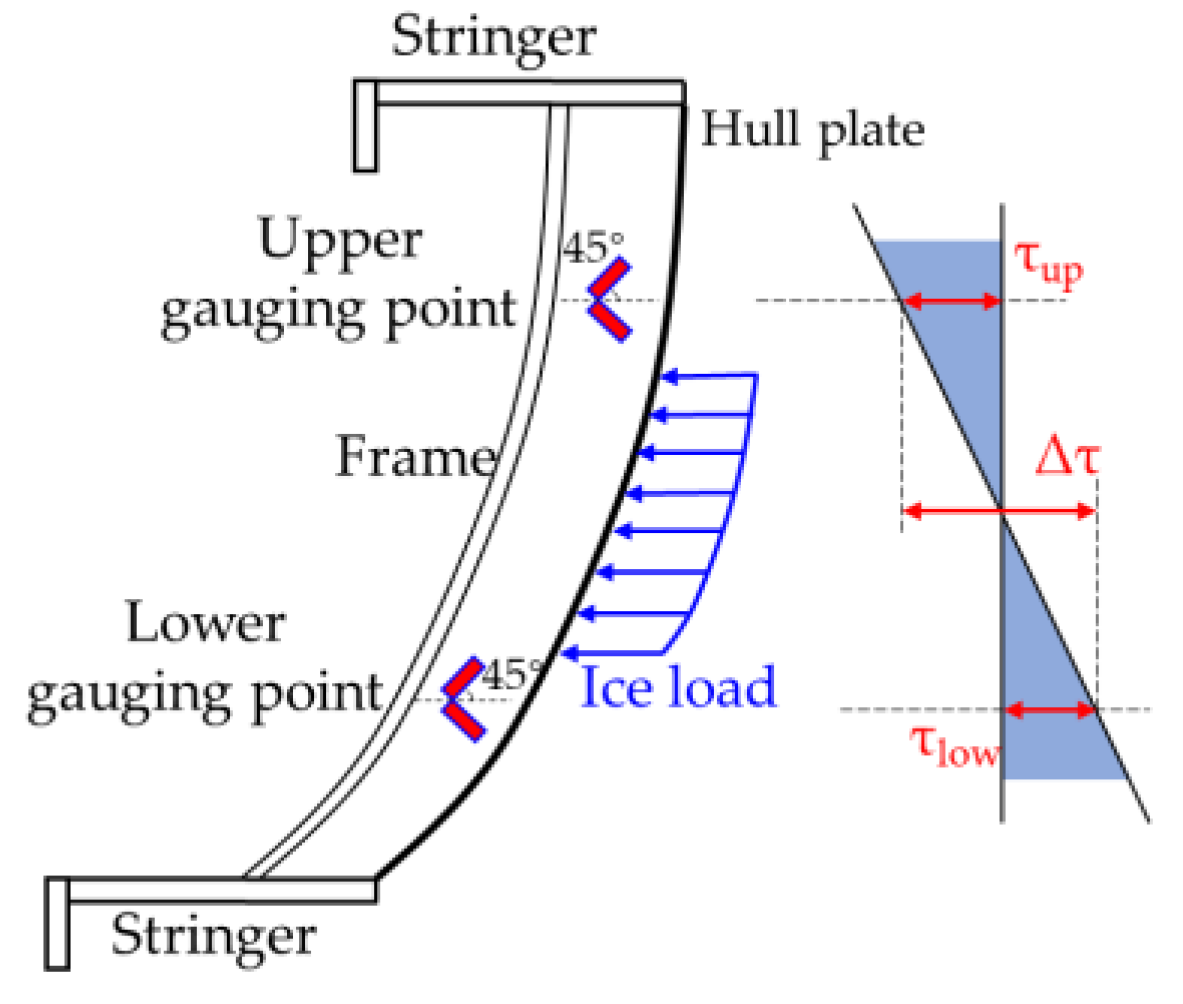
3.1.3. Local Ice Load Identification Method

Due to the intense collision, compression, and friction of sea ice, it is a significant challenge to directly install sensors on the hull structure for the purpose of measuring local ice loads. Consequently, the commonly adopted approach is to install strain sensors on the frames or outer plate near the area of sea ice collision. By utilizing the strain–stress relationship, direct calculation method, or load identification methods, the ice loads exerted on the hull structure are indirectly measured [33].
The current research primarily employs the influence coefficient matrix method (ICM) to establish the transformation relationship between measured shear strains and localized ice loads [34]. This methodology offers significant advantages through its simplified matrix formulation while effectively accounting for strain contributions from adjacent loading zones [35]. The approach demonstrates remarkable computational efficiency for real-time applications without compromising identification accuracy, making it particularly suitable for polar vessel structural monitoring systems where both processing speed and measurement precision are critical operational requirements. The methodology establishes a quantitative relationship between ice-induced loads and structural shear strain responses through the following mathematical formulation:
[ C ] m × m { Δ γ ( t ) } m × 1 = { F ice ( t ) } m × 1
where [ C ] is the influence coefficient matrix between strain and ice load; Δ γ is the shear strain difference values at each frame; F ice is the ice load of each frame; and m is the number of monitoring areas. The influence coefficient matrix elements are determined through systematic application of normal loads to individual sub-regions, with each loading case producing corresponding shear strain responses at measurement points that collectively populate the matrix terms during the inversion process.

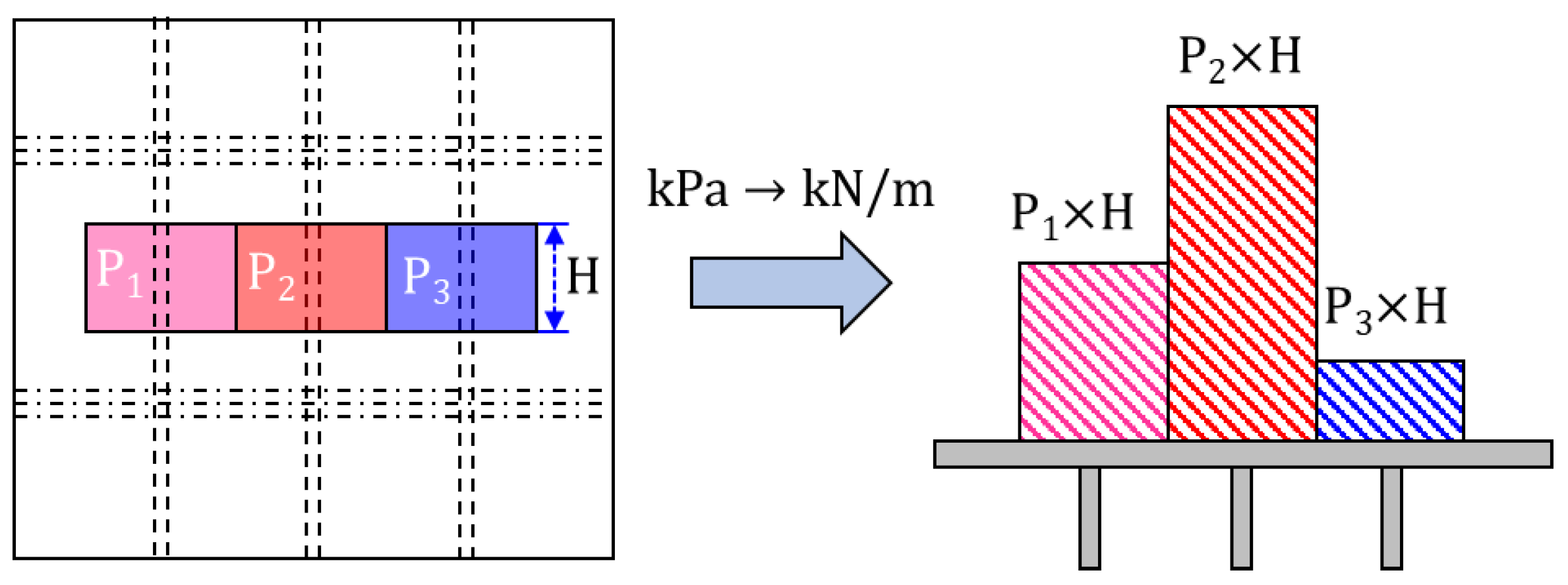
3.1.4. Simplification of Local Ice Loads

The influence coefficient matrix method operates under two fundamental assumptions concerning ice load characteristics. Primarily, the approach presumes quasi-static loading conditions, effectively neglecting dynamic impact effects by modeling ice pressure as gradually applied to the ship structure [36]. Secondly, the method assumes uniform pressure distribution across the designated contact area. Consequently, the identified ice load is represented as distributed pressure, which is conventionally transformed into equivalent linear load representations for analytical purposes in this research domain [37]. This pressure-to-line-load conversion methodology is schematically illustrated in Figure 10, demonstrating the fundamental load transformation process employed in the analysis.

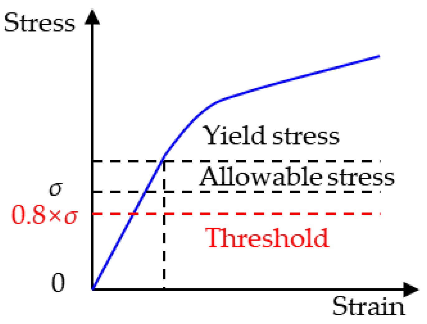
3.1.5. Local Ice Load Assessment

Unlike the extensive numerical simulations needed for global structural analysis, the assessment of local structures primarily focuses on evaluating specific components’ capacity to resist anticipated stress concentrations. This approach emphasizes direct load effects on critical sections while deliberately excluding broader environmental factors like wind, wave, and current actions [38,39]. For Arctic marine structures, ice loading emerges as the dominant design consideration, rendering other environmental loads secondary in structural integrity evaluations. Consequently, the numerical modeling of local structural components is typically simplified to consider ice load effects exclusively, providing a more efficient yet conservative design framework for ice-prone environments.
Numerical simulation provides an effective approach for comprehensive structural stress analysis, enabling the precise identification of stress concentrations at critical locations and potential hotspots. The China Classification Society (CCS) “Guidelines for Hull Monitoring and Decision-Support Systems for Ice Operations” specifies allowable stress thresholds for key structural components in Ice Class B3 to B1* vessels under ice loading conditions [40]. The schematic representation of the threshold values is illustrated in Figure 11. A safety evaluation index is established by calculating the ratio between numerically determined stress values and the predefined safety threshold. The warning system is activated when this index reaches or exceeds 0.8 (indicating imminent plastic deformation). These established stress limits serve as valuable benchmarks for developing ice load warning criteria and assessing structural integrity during ice–structure interactions.

3.2. Full-Scale Data and Numerical Analysis

3.2.1. Full-Scale Data Source

The full-scale data were obtained from the 2019 operational records of the M/V Tianen [41], corresponding to the same voyage as the sea ice image dataset described in Section 2. Due to structural constraints preventing strain sensor installation in the ship–ice interaction zone (located at the anti-heeling water tank), the monitoring area was strategically positioned at the portside bosun’s store outer plating in the far-field [42]. Figure 12 illustrates the spatial relationship between the actual ice-impact zone and the instrumented monitoring zone.

3.2.2. Local Structural Numerical Model

The finite element model of the structure was developed based on actual ship design drawings, incorporating key structural components, including the outer hull plating, inner decks, longitudinal, frames, as well as local reinforcements and brackets. The entire model was discretized using shell elements, with EH36 high-strength steel (yield stress = 355 MPa) specified for all hull structural members to accurately represent the material properties. Figure 13 depicts the local finite element model of the bow of M/V Tianen.

3.2.3. Numerical Model Calibration

Accurate FEM model plays a critical role in ice load identification and numerical calculation, with model calibration representing an essential phase of this process [23]. In the present study, the frame structure was systematically loaded using a manually operated hoist system, while high-precision strain sensors continuously monitored the shear strain response. This experimental configuration enabled comprehensive validation through direct comparison between finite element simulation results and empirical measurements. As demonstrated in Figure 14, the close agreement between numerical predictions and experimental data confirms the validity of the developed finite element model for ice load assessment applications. The calibration procedure not only verified model accuracy but also established a reliable foundation for subsequent ice load assessment.

3.3. Case Study and Discussion

This study validates the effectiveness of the monitoring system by analyzing data from two typical sea ice scenarios. Scenario 1 involves the ship colliding with small ice floe, which is crushed into smaller pieces due to the extrusion pressure. In Scenario 2, the ship encounters an ice cake and experience forces causing inversion and slip, but without the ice breaking apart. The environmental parameters for these two scenarios are detailed in Table 2.
The actual monitoring system follows the data processing flow depicted in Figure 15. The process begins with data preprocessing (Step 1), where Kalman filtering and bandpass filtering techniques are employed to mitigate signal noise and eliminate baseline drift in the high-frequency and long-duration acquisition data. The processed data then undergo numerical computation to derive the influence coefficient matrix (Step 2), which enables ice load identification expressed as contact pressure distributions. These pressure profiles are subsequently simplified into equivalent line loads (Step 3) to serve as boundary conditions for finite element analysis. Step 4 involves both the computation of von Mises stress contours and post-processing to extract hotspot stresses at critical structural components. Finite element analysis is based on the commercial software ABAQUS 2020, with approximately 150,000 elements. When calculated on Intel i5-14400F hardware (Intel Corporation, Santa Clara, CA, USA), the computation time is less than 1 min, which can basically meet the real-time requirements of the monitoring system. Ice load assessment (Step 5) is performed by comparing the finite element results against allowable stress thresholds (set at 80% of the code-specified values) derived from classification society formulas. The analysis demonstrates that under icebreaker-escorted conditions, the encountered ice loads in typical scenarios remain well below critical levels, revealing substantial design margins in the merchant vessel’s ice-strengthened structures. Notably, Scenario 2 involving small ice fragments shows negligible structural impact, confirming that operational attention should primarily focus on large ice floes during actual navigation.

4. Conclusions

This study proposes an innovative monitoring system designed to track sea ice conditions and quantify local ice loads on polar-class cargo vessels, with dual objectives of assessing structural impacts and ensuring safe navigation in ice-covered waters. The system integrates a high-precision sea ice recognition model based on the DeepLab v3+ framework, which achieves over 90% accuracy in ice concentration identification using historical ice image datasets, providing real-time navigational guidance that effectively complements large-scale remote sensing data. For localized ice load analysis, we developed a comprehensive monitoring–identification–assessment framework combining numerical simulation, full-scale measurement, and classification society calculation methods, enabling the quantitative evaluation of structural responses to ice loads. Detailed case studies demonstrate the system’s analytical workflow. As a representative implementation of hull health monitoring for polar vessels, this integrated solution shows significant potential for broad application in commercial Arctic shipping operations.
Sea ice and the resulting ice loads represent unique environmental hazards for vessels navigating ice-covered waters. The quantitative characterization of both ice parameters and their structural impacts provides critical operational guidance for ship handlers, while the accumulated dataset of ice conditions and corresponding load responses offers valuable support for structural design optimization and ice navigation safety assurance. Building upon this expanded dataset, future research should prioritize investigating the parameter influence mechanisms of sea ice interactions and developing reliable short-term prediction models to enhance real-time decision-making capabilities.

Author Contributions

J.J. and S.J. conceptualized this study; J.J. and S.H. carried out this study, performed the calculations, and drafted the paper; H.J., X.C., and S.J. processed the review and editing of the paper. All authors have read and agreed to the published version of the manuscript.

Funding

This research was supported by National Key Research and Development Program of China (Grant No. 2024YFC2816403), the National Natural Science Foundation of China (Grant Nos. 52101300, 52192693, 52192690, and 42176241), Social Development Science and Technology Project of Shanghai Science and Technology Innovation Plan (22DZ1204500), and Special Project of Ministry of Industry and Information Technology of China (Grant No. 2021-342).

Data Availability Statement

The data presented in this study are available on request from the corresponding authors.

Acknowledgments

The authors would like to thank COSCO Shipping Specialized Carriers Co., Ltd., for the support of full-scale measurement.

Conflicts of Interest

Authors Jinhui Jiang and Herong Jiang were employed by the company Shanghai Ship and Shipping Research Institute Co., Ltd. The remaining authors declare that the research was conducted in the absence of any commercial or financial relationships that could be construed as a potential conflict of interest.

Abbreviations

The following abbreviations are used in this manuscript:
M/VMerchant Vessel
SHMStructural health monitoring
SVMSupport vector machine
DVRDigital video storage
HDHigh-definition
DCNNDeep Convolutional Neural Network
IoUIntersection over Union
UIWLUpper ice waterline
LIWLLower ice waterline
ICMInfluence coefficient matrix method
CCSChina Classification Society

References

  1. Ebinger, C.K.; Zambetakis, E. The geopolitics of Arctic melt. Int. Aff. 2009, 85, 1215–1232. [Google Scholar] [CrossRef]
  2. Pang, X.; Zhang, C.; Ji, Q.; Chen, Y.; Zhu, Z.; Zhu, Y.; Yan, Z. Analysis of sea ice conditions and navigability in the Arctic Northeast Passage during the summer from 2002–2021. Geo-Spat. Inf. Sci. 2023, 26, 465–479. [Google Scholar] [CrossRef]
  3. Zhang, Y.; Meng, Q.; Ng, S.H. Shipping efficiency comparison between Northern Sea Route and the conventional Asia-Europe shipping route via Suez Canal. J. Transp. Geogr. 2016, 57, 241–249. [Google Scholar] [CrossRef]
  4. Hu, B.; Liu, L.; Wang, D. Prediction of performance of a non-icebreaking ship in marginal ice zone. J. Hydrodyn. 2022, 34, 93–103. [Google Scholar] [CrossRef]
  5. Fu, S.; Zhang, D.; Montewka, J.; Yan, X.; Zio, E. Towards a probabilistic model for predicting ship besetting in ice in Arctic waters. Reliab. Eng. Syst. Saf. 2016, 155, 124–136. [Google Scholar] [CrossRef]
  6. Min, R.; Liu, Z.; Pereira, L.; Yang, C.; Sui, Q.; Marques, C. Optical fiber sensing for marine environment and marine structural health monitoring: A review. Opt. Laser Technol. 2021, 140, 107082. [Google Scholar] [CrossRef]
  7. Okasha, N.M.; Frangopol, D.M.; Decò, A. Integration of structural health monitoring in life-cycle performance assessment of ship structures under uncertainty. Mar. Struct. 2010, 23, 303–321. [Google Scholar] [CrossRef]
  8. Reed, H.M.; Earls, C.J. Stochastic identification of the structural damage condition of a ship bow section under model uncertainty. Ocean Eng. 2015, 103, 123–143. [Google Scholar] [CrossRef]
  9. Decò, A.; Frangopol, D.M. Real-time risk of ship structures integrating structural health monitoring data: Application to multi-objective optimal ship routing. Ocean Eng. 2015, 96, 312–329. [Google Scholar] [CrossRef]
  10. Zambon, A.; Moro, L.; Brown, J.; Kennedy, A.; Oldford, D. A Measurement System to Monitor Propulsion Performance and Ice-Induced Shaftline Dynamic Response of Icebreakers. J. Mar. Sci. Eng. 2022, 10, 522. [Google Scholar] [CrossRef]
  11. Turnbull, I.D.; Bourbonnais, P.; Taylor, R.S. Investigation of two pack ice besetting events on the Umiak I and development of a probabilistic prediction model. Ocean Eng. 2019, 179, 76–91. [Google Scholar] [CrossRef]
  12. Seymour, W.L.; Katharine, A.G.; Andy, L.R.; Duncan, J.W. CryoSat-2 estimates of Arctic sea ice thickness and volume. Geophys. Res. Lett. 2013, 40, 732–737. [Google Scholar]
  13. Aldenhoff, W.; Berg, A.; Eriksson, L.E.B. Sea Ice Concentration Estimation from Sentinel-1 Synthetic Aperture Radar Images over the Fram Strait; IEEE International Geoscience and Remote Sensing Symposium (IGARSS): Beijing, China, 2016; pp. 7675–7677. [Google Scholar]
  14. Weissling, B.; Ackley, S.; Wagner, P.; Xie, H. EISCAM-Digital image acquisition and processing for sea ice parameters from ships. Cold Reg. Sci. Technol. 2009, 57, 49–60. [Google Scholar] [CrossRef]
  15. Toyota, T.; Haas, C.; Tamura, T. Size distribution and shape properties of relatively small sea-ice floes in the Antarctic marginal ice zone in late winter. Deep Sea Res. Part II Top. Stud. Oceanogr. 2011, 58, 1182–1193. [Google Scholar] [CrossRef]
  16. Zhang, Q.; Skjetne, R.; Metrikin, I.; Løset, S. Image processing for ice floe analyses in broken-ice model testing. Cold Reg. Sci. Technol. 2015, 111, 27–38. [Google Scholar] [CrossRef]
  17. Chi, J.; Kim, H. Prediction of Arctic sea ice concentration using a fully data driven deep neural network. Remote Sens. 2017, 9, 1305. [Google Scholar] [CrossRef]
  18. Kalke, H.; Loewen, M. Support vector machine learning applied to digital images of river ice conditions. Cold Reg. Sci. Technol. 2018, 155, 225–236. [Google Scholar] [CrossRef]
  19. Yan, Q.; Huang, W. Detecting sea ice from techdemosat-1 data using support vector machines with feature selection. IEEE J. Sel. Top. Appl. Earth Obs. Remote Sens. 2019, 12, 1409–1416. [Google Scholar] [CrossRef]
  20. Kim, D.H.; Nam, J.H. Determination of the lower boundary of a rotating ice patch for ice thickness estimation using image convolution and machine learning. Cold Reg. Sci. Technol. 2020, 173, 103009. [Google Scholar] [CrossRef]
  21. Böhm, A.M.; von Bock und Polach, R.U.F.; Herrnring, H.; Ehlers, S. The measurement accuracy of instrumented ship structures under local ice loads using strain gauges. Mar. Struct. 2021, 76, 102919. [Google Scholar] [CrossRef]
  22. Suyuthi, A.; Leira, B.J.; Riska, K. Short term extreme statistics of local ice loads on ship hulls. Cold Reg. Sci. Technol. 2012, 82, 130–143. [Google Scholar] [CrossRef]
  23. Suominen, M.; Kujala, P.; Romanoff, J.; Remes, H. Influence of load length on short-term ice load statistics in full-scale. Mar. Struct. 2017, 52, 153–172. [Google Scholar] [CrossRef]
  24. Li, F.; Goerlandt, F.; Kujala, P.; Lensu, M. Evaluation of selected state-of-the-art methods for ship transit simulation in various ice conditions based on full-scale measurement. Cold Reg. Sci. Technol. 2018, 151, 94–108. [Google Scholar] [CrossRef]
  25. Choi, J.; Park, G.; Kim, Y.; Jang, K.; Park, S.; Ha, M.; Han, Y.; Iyerusalimskiy, A.; St John, J. Ice Load Monitoring System for Large Arctic Shuttle Tanker. In Proceedings of the International Conference on Ship and Offshore Technology, Busan, Republic of Korea, 28–29 September 2009. [Google Scholar]
  26. Leira, B.; Børsheim, L.; Espeland, Ø.; Amdahl, J. Ice-load estimation for a ship hull based on continuous response monitoring. J. Eng. Marit. Environ. 2009, 223, 529–540. [Google Scholar] [CrossRef]
  27. Wang, Q.; Lu, P.; Zu, Y.; Li, Z.; Leppäranta, M.; Zhang, G. Comparison of Passive Microwave Data with Shipborne Photographic Observations of Summer Sea Ice Concentration along an Arctic Cruise Path. Remote Sens. 2019, 11, 2009. [Google Scholar] [CrossRef]
  28. Zhang, C.; Chen, X.; Ji, S. Semantic image segmentation for sea ice parameters recognition using deep convolutional neural networks. Int. J. Appl. Earth Obs. Geoinf. 2022, 112, 102885. [Google Scholar] [CrossRef]
  29. Lensu, M.; HÄanninen, S. Short term monitoring of ice loads experienced by ships. In Proceedings of the 17th International Conference on Port and Ocean Engineering under Arctic Conditions, Trondheim, Norway, 16–19 June 2003. [Google Scholar]
  30. Kubiczek, J.M.; Andresen-Paulsen, G.; Herrnring, H.; von Bock und Polach, F.; Ehlers, S. Development of a design load patch for the consideration of ice loads. Ships Offshore Struct. 2020, 15, 20–28. [Google Scholar] [CrossRef]
  31. Liu, L.; Ji, S. Comparison of sphere-based and dilated-polyhedron-based discrete element methods for the analysis of ship–ice interactions in level ice. Ocean Eng. 2022, 244, 110364. [Google Scholar] [CrossRef]
  32. Kong, S.; Cui, H.Y.; Tian, Y.; Ji, S. Identification of ice loads on shell structure of ice-going vessel with Green kernel and regularization method. Mar. Struct. 2020, 74, 102820. [Google Scholar] [CrossRef]
  33. Yamauchi, Y.; Mizuno, S.; Tsukuda, H. The icebreaking performance of Shirase in the maiden Antarctic voyage. In Proceedings of the International Offshore and Polar Engineering Conference, Maui, HI, USA, 19–24 June 2011. [Google Scholar]
  34. Suominen, M.; Kujala, P.; Romanoff, J.; Remes, H. The effect of the extension of the instrumentation on the measured ice-induced load on a ship hull. Ocean Eng. 2017, 144, 327–339. [Google Scholar] [CrossRef]
  35. Kwon, Y.H.; Lee, T.K.; Choi, K. A study on measurements of local ice pressure for ice breaking research vessel “ARAON” at the Amundsen Sea. Int. J. Nav. Archit. Ocean Eng. 2015, 7, 490–499. [Google Scholar] [CrossRef]
  36. Ritch, R.; Frederking, R.; Johnston, M.; Browne, R.; Ralph, F. Local ice pressures measured on a strain gauge panel during the CCGS Terry Fox bergy bit impact study. Cold Reg. Sci. Technol. 2008, 52, 29–49. [Google Scholar] [CrossRef]
  37. Adams, J.M.; Valtonen, V.; Kujala, P. Validation of the line-like nature of ice-induced loads using an inverse method. In Proceedings of the 25th International Conference on Port and Ocean Engineering under Arctic Conditions, Delft, The Netherlands, 9–13 June 2019. [Google Scholar]
  38. Huang, L.; Tuhkuri, J.; Igrec, B.; Li, M.; Stagonas, D.; Toffoli, A.; Cardiff, P.; Thomas, G. Ship resistance when operating in floating ice floes: A combined CFD&DEM approach. Mar. Struct. 2020, 74, 102817. [Google Scholar]
  39. Mohapatra, S.C.; Amouzadrad, P.; Bispo, I.B.d.S.; Soares, C.G. Hydrodynamic Response to Current andwind on a Large Floating Interconnected Structure. J. Mar. Sci. Eng. 2025, 13, 63. [Google Scholar] [CrossRef]
  40. CCS. Guidelines for Hull Monitoring and Assistant Decision-Making System for Operations in Ice; China Classification Society: Beijing, China, 2018. [Google Scholar]
  41. He, S.; Chen, X.; Kong, S.; Ji, S. Measurement and identification of ice loads on hull structures in far field based on dynamic effects. Chin. J. Ship Res. 2021, 16, 54–63. [Google Scholar]
  42. Wang, J.; Chen, X.; Sun, K.; Ji, S. Far-field identification of ice loads on ship structures by radial basis function neural network. Ocean Eng. 2023, 282, 115072. [Google Scholar] [CrossRef]
Figure 1. Ship-based camera layout scheme.
Jmse 13 00808 g001
Figure 2. The connection diagram of the sea ice image monitoring device.
Jmse 13 00808 g002
Figure 3. Sea ice concentration identification model based on DeepLab V3+.
Jmse 13 00808 g003
Figure 4. Dataset source: (a) route of the 2018 and 2019 arctic voyage; (b) sea ice image.
Jmse 13 00808 g004
Figure 5. Segmentation results of sea ice images: (a) original image (b) segmentation results.
Jmse 13 00808 g005
Figure 6. Sea ice concentration time history curve: (a) M/V Tianyou 2018; (b) M/V Tianen 2019.
Jmse 13 00808 g006
Figure 7. The research framework for ice load acquisition and assessment.
Jmse 13 00808 g007
Figure 8. Numerical simulation result of typical ice navigation conditions.
Jmse 13 00808 g008
Figure 9. Shear strain measurement diagram of frames.
Jmse 13 00808 g009
Figure 10. Schematic diagram of the conversion method from ice pressure to line load.
Jmse 13 00808 g010
Figure 11. The schematic representation of the threshold values.
Jmse 13 00808 g011
Figure 12. The spatial relationship between the actual ice-impact zone and the instrumented monitoring zone.
Jmse 13 00808 g012
Figure 13. The local finite element model of the bow.
Jmse 13 00808 g013
Figure 14. Tensile test of frame structure: (a) test diagram; (b) time history curve of load and strain; (c) comparison of test results and finite element results.
Jmse 13 00808 g014
Figure 15. The data processing flow of two typical scenarios.
Jmse 13 00808 g015
Table 1. The identification evaluation data of the validation set.
Parameters I o U -Sea (%) I o U -Ice (%) I o U -Sky (%) I o U -Ship (%) m I o U (%)
Testing set82.3593.1887.7599.4390.68
Table 2. Environmental parameters of typical sea ice scenarios.
No.DateUTC TimeShip Speed (m/s)Draft (m)Ice TypeIce Thickness (m)Ice Failure Pattern
12 August 201912:025.146.5Ice floe1.2Compression
23 August 20193:084.246.5Ice cake1.5Inversion and slip
Disclaimer/Publisher’s Note: The statements, opinions and data contained in all publications are solely those of the individual author(s) and contributor(s) and not of MDPI and/or the editor(s). MDPI and/or the editor(s) disclaim responsibility for any injury to people or property resulting from any ideas, methods, instructions or products referred to in the content.

