A Novel Method for Inverting Deep-Sea Sound-Speed Profiles Based on Hybrid Data Fusion Combined with Surface Sound Speed

Abstract

Sound speed profiles (SSPs) must be detected simultaneously to perform a multibeam depth survey. Accurate real-time sound speed profile (SSP) acquisition remains a critical challenge in deep-sea multibeam bathymetry due to the limitations regarding direct measurements under harsh operational conditions. To address the issue, we propose a joint inversion framework integrating World Ocean Atlas 2023 (WOA23) temperature–salinity model data, historical in situ SSPs, and surface sound speed measurements. By constructing a high-resolution regional sound speed field through WOA23 and historical SSP fusion, this method effectively mitigates spatiotemporal heterogeneity and seasonal variability. The artificial lemming algorithm (ALA) is introduced to optimize the inversion of empirical orthogonal function (EOF) coefficients, enhancing global search efficiency while avoiding local optimization. An experimental validation in the northwest Pacific Ocean demonstrated that the proposed method has a better performance than that of conventional substitution, interpolation, and WOA23-only approaches. The results indicate that the mean absolute error (MAE), root mean square error (RMSE), and maximum error (ME) of SSP reconstruction are reduced by 41.5%, 46.0%, and 49.4%, respectively. When the reconstructed SSPs are applied to multibeam bathymetric correction, depth errors are further reduced to 0.193 m (MAE), 0.213 m (RMSE), and 0.394 m (ME), effectively suppressing the “smiley face” distortion caused by sound speed gradient anomalies. The dynamic selection of the first six EOF modes balances computational efficiency and reconstruction fidelity. This study provides a robust solution for real-time SSP estimation in data-scarce deep-sea environments, particularly for underwater autonomous vehicles. This method effectively mitigates the seabed distortion caused by missing real-time SSPs, significantly enhancing the accuracy and efficiency of deep-sea multibeam surveys.

1. Introduction

The accurate acquisition of seawater sound-speed profiles (SSPs) is critical for high-precision deep-sea multibeam bathymetry [1,2,3,4]. The most direct method of obtaining an SSP is through on-site observations. However, this approach is time-consuming and labor-intensive. Moreover, due to the spatiotemporal variability of sound speed, these on-site observations cannot provide real-time SSPs over a large area. In recent years, vertical marine observation data (including ship-based measurements and fixed-point observations at SSP stations, moorings, and buoys) have significantly increased. The World Ocean Atlas 2023 (WOA23) is one of the most authoritative and comprehensive marine temperature–salinity datasets internationally, widely used in marine science and related research fields. By integrating marine observation data from around the globe, and after stringent quality control and interpolation processing, this dataset can provide high-precision information on the distribution of marine temperature and salinity. These data provided the basic marine environmental background for this study, aiding in the analysis of marine physical properties and their impact on related phenomena [5]. Nevertheless, the spatial resolution of existing vertical observation data remains relatively low, and these data cannot be used to describe the internal structural changes in the ocean in real time. On the other hand, due to the diversity of marine environmental changes, the surface sound speed of seawater is greatly affected by seasons, climate, and sea surface temperature. There is a significant difference between historical SSP data and the actual environment, which cannot meet the needs of real-time sound-speed correction in multibeam measurements. Therefore, combining the surface sound speed measured by the multibeam system with the historical SSP data in the survey area to invert the real-time SSP on-site is a good solution.

To address the issue of the real-time inversion of SSPs, the academic community has proposed a variety of theories and methods. In early research, LeBlanc and Middleton [6] constructed an underwater sound-speed data model, using statistical methods to predict SSPs, but they did not consider the spatiotemporal dynamic changes. Davis [7] proposed a climate-state prediction model based on the correlation between the sea surface temperature and sound speed, laying the foundation for subsequent data assimilation research. With the development of the empirical orthogonal function (EOF) method, Shen et al. [8] first introduced the EOF into the reconstruction of shallow-water SSPs, verifying the effectiveness of its dimensionality reduction representation. Ding et al. [9] further applied it to multibeam measurements, proposing a method for constructing the sound-speed field based on the interpolation of EOF coefficients. However, due to data sparsity, the error in deep-sea scenarios was significant.

In recent years, the combination of data-driven approaches and optimization algorithms has become a research hotspot. Zhang et al. [10] utilized the EOF to reconstruct deep-sea SSPs and combined multibeam data to verify the accuracy of the correction, but they did not solve the problem of the dynamic adaptation of surface sound speed. Huang et al. [11] proposed a method for reconstructing the full-depth SSP, reducing the shallow layer error to 0.2 m/s through stratified error control; however, this method relied on dense real-measurement data. In terms of optimization algorithms, Zhang et al. [12] used a simulated annealing algorithm to invert the SSPs, enhancing the global search capability; however, the convergence speed was relatively slow. Li et al. [13] combined the matched field with neural networks to construct the sound-speed time field, achieving sound-speed prediction in complex sea areas; however, the model generalization was insufficient. In international research, Capell [14] used multibeam data to invert the error of the SSP, revealing the impact of the sound-speed gradient on the depth measurement accuracy, and providing an important reference for error control. Mohammadloo [15] successfully inverted the SSPs by minimizing the difference between multibeam overlapping data using Differential Evolution (DE) and Gauss–Newton (GN) optimization algorithms. However, the existing methods still have two major limitations: firstly, they rely solely on model data (such as WOA23) or historical measured data, lacking adaptability to the dynamic changes in surface sound speed; secondly, traditional optimization algorithms (such as genetic algorithms) tend to fall into local optima during the inversion process, resulting in insufficient reconstruction accuracy.

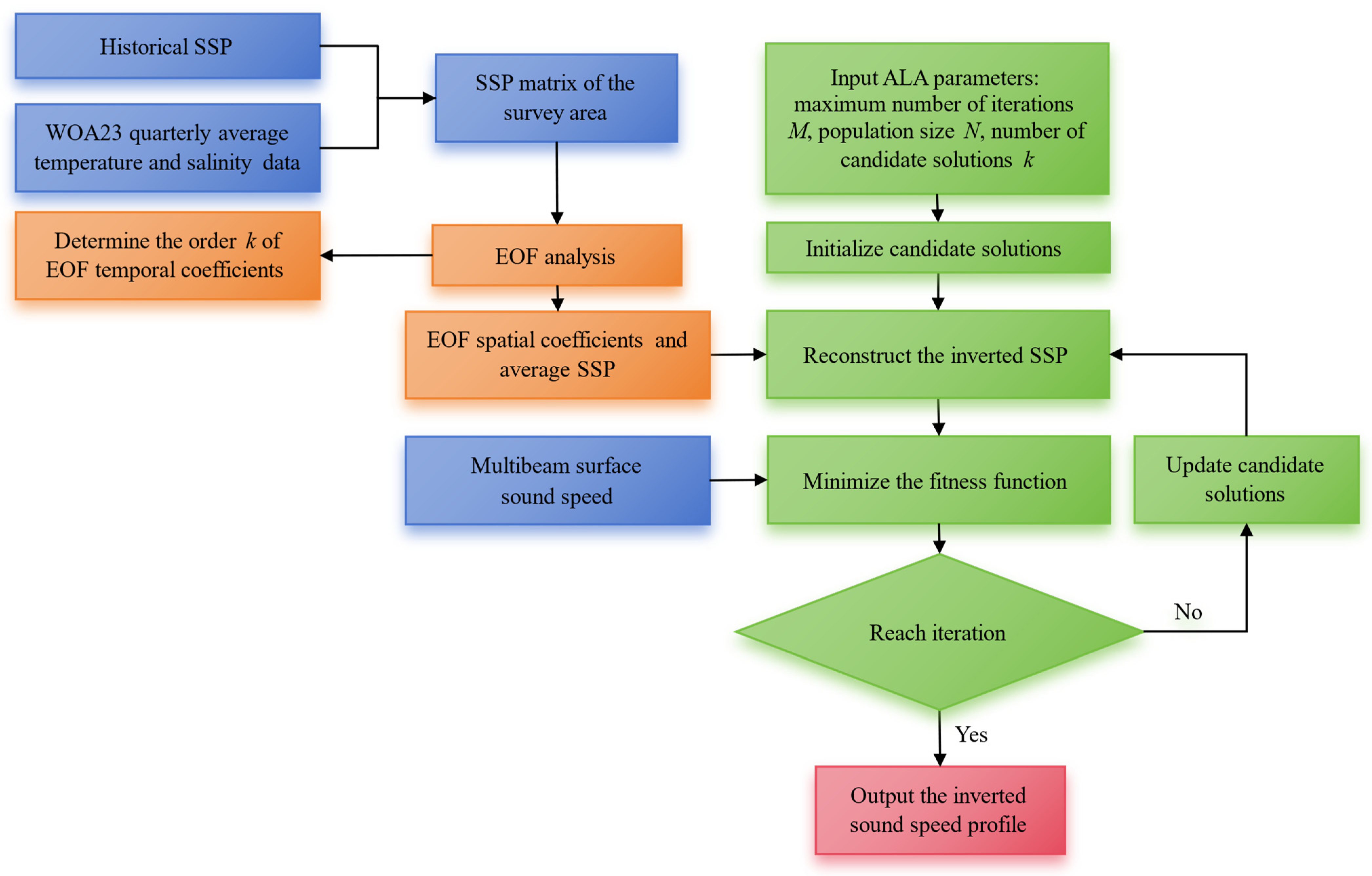
This study proposes a novel approach for sound-speed profile inversion in uncharted deep-sea regions by integrating the high-resolution WOA23 dataset with limited historical in situ measurements. A fitness function is formulated to quantify the discrepancy between real-time surface sound-speed data acquired by multibeam systems and the inverted SSPs, thereby enhancing temporal coherence with field observations and improving the inversion accuracy. The artificial lemming algorithm (ALA), renowned for its global optimization efficiency, is employed to establish a rapid and robust SSP inversion framework. The accuracy and practical utility of the inverted profiles are rigorously evaluated using a constant-gradient acoustic ray-tracing model. Validation with measured multibeam bathymetric data further confirms the method’s validity and feasibility, demonstrating its critical reference value for real-world applications in autonomous underwater vehicle navigation and high-precision seabed mapping.

The remaining content of the paper is organized as follows: Section 2 details the EOF representation principles, ALA, and joint inversion workflow. Section 3 describes the experimental data and evaluation metrics. Section 4 presents the SSP reconstruction accuracy and bathymetric correction results, while Section 5 concludes with future research directions.

2. Methods

2.1. EOF Representation Principle of SSPs

2.1.1. EOF Representation of SSPs

The EOF analysis method, also known as the principal component analysis method, decomposes the SSP matrix composed of SSPs in a certain area into orthogonal time vectors and spatial vectors [16,17,18,19], obtaining basis functions. The first few EOFs can represent any SSP in the area. The SSP matrix $C_{M\times N}$, given by Equation (1), collected in a certain sea area consists of N SSPs that are interpolated into M vertical standard layers to obtain the sound-speed matrix:

$$C_{M\times N}=\left[\begin{array}{cccc}{c}_1(1)& c_2(1)& \dots & c_N(1)\\ c_1(2)& c_2(2)& \dots & c_N(2)\\ ⋮& ⋮& \ddots & ⋮\\ c_1(M)& c_2(M)& \dots & c_N(M)\end{array}\right]$$

(1)

where each column is a standard layer interpolation of an SSP, each row is the sound-speed value of all SSPs at the same standard layer, and $c(i)$ is the i-th row of the sound-speed matrix. The average value of each row in the sound-speed matrix is taken to obtain the average sound-speed matrix given by

$${\overline{C}}_{M\times N}={\displaystyle \frac{1}{M}}{\displaystyle \sum _{i=1}^{M}c(i)}$$

(2)

The sound-speed matrix is subtracted from the average sound-speed matrix column by column to obtain the perturbation matrix of each SSP relative to the average SSP, which is expressed as

$$\Delta C_{M\times N}=C_{M\times N}-{\overline{C}}_{M\times N}$$

(3)

Its covariance matrix is

$$R_{M\times M}={\displaystyle \frac{\Delta C_{M\times N}\Delta C_{M\times N}^T}{N}}$$

(4)

The eigenvalue decomposition of $R_{M\times M}$ is calculated by

$$R_{M\times M}{F}_{M\times M}=D_{M\times M}{F}_{M\times M}$$

(5)

where $D_{M\times M}$ is the eigenvalue matrix. $F_{M\times M}$ is the matrix of eigenvectors corresponding to the eigenvalues, which is the EOF spatial function.

Projecting EOF into $\Delta C_{M\times N}$, the time coefficients $A_{M\times N}$ corresponding to all spatial characteristic vectors can be obtained by

$$A_{M\times N}=F_{M\times M}^T\Delta C_{M\times N}$$

(6)

where each row of $A_{M\times N}$ is the time coefficient corresponding to each characteristic vector. Finally, the EOF representation form of the SSP is

$$C_{M\times N}={\overline{C}}_{M\times N}+F_{M\times M}{A}_{M\times N}$$

(7)

Arranging the eigenvalues in descending order, taking the first few EOFs can more accurately represent the sample SSP. A certain SSP can be represented by the first k EOFs as

$$c(z)=c_0(z)+{\displaystyle \sum _{i=1}^k{t}_i{f}_i(z)}$$

(8)

where z is the depth value, $c_0\left(z\right)$ is the average SSP, $c\left(z\right)$ is the SSP represented by EOF, k is the EOF order, $t_i$ is the EOF coefficient, and $f_i\left(z\right)$ is the empirical orthogonal function.

From Equation (8), it is known that $c\left(z\right)$ and $t_i$ correspond one-to-one. When correcting the SSP, only the first few EOF coefficients need to be fine-tuned, which greatly reduces the number of parameters to be searched. Therefore, the process of solving the optimal SSP is transformed into the process of searching for a group of optimal EOF coefficients.

2.1.2. Selection of EOF Order for SSP Reconstruction

According to the above method, EOF decomposition is performed to extract spatial functions and time functions, and the variance contribution rate and cumulative variance contribution rate of each EOF order are calculated. The variance contribution rate represents the percentage of sound field information contained in each EOF order, and its calculation formula is

$${\sigma }_i={\displaystyle \frac{{\lambda }_i}{{\displaystyle \sum _{i=1}^M{\lambda }_i}}}\times 100\%$$

(9)

where ${\sigma }_i$ represents the variance contribution rate of the i-th order and ${\lambda }_i$ represents the i-th eigenvalue in the eigenvalue matrix, arranged in descending order.

The cumulative contribution rate of the first k EOF order is expressed as

$$w(k)={\displaystyle \sum _{i=1}^k{\lambda }_i}/{\displaystyle \sum _{j=1}^M{\lambda }_j}$$

(10)

It is generally believed that, if the value of $w(k)$ is greater than or equal to 95%, then using the first k EOFs can better represent the main SSP information in the area [20].

2.2. Artificial Lemming Algorithm

The ALA is a novel metaheuristic optimization framework introduced in January 2025 [21]. To address the problems of premature convergence and the difficulty of maintaining a robust balance between exploration and development that other metaheuristic algorithms often face, ALA introduces a new energy-reduction mechanism that dynamically adjusts this balance throughout the optimization process, significantly improving its robustness and effectiveness across different optimization landscapes. In addition, ALA uniquely integrates Brownian motion and Lévy flight into its search strategy, enabling it to move away from local optimality and improve global search capabilities.

The algorithm is based on the characteristics of lemmings, whose main habits include long-distance migration, digging holes, foraging for food, and evading natural predators. ALA mainly simulates the above four behaviors of lemmings. In the first behavior, when the lemming population is too large and food is scarce, the lemming will randomly migrate long distances. Here, lemmings will explore the search space according to the current location and the location of random individuals in the population, looking for habitats rich in food resources, so as to obtain better living conditions and resources. At the same time, it is worth noting that the direction and distance of lemming migration are not static, and are affected by many factors, such as ecological environment. The second behavior of lemmings is to burrow into their habitat, forming complex tunnels that provide them with safe shelter and a place to store food. The lemmings will randomly dig new burrows based on the current location of the burrow and the location of random individuals in the population. This design helps them escape predators quickly and find food more efficiently. In the third behavior, lemmings move widely and randomly within burrows in their habitat, relying on their keen sense of smell and hearing to locate food sources. Lemmings usually establish a relatively small feeding area within their habitat, depending on the abundance and availability of food. In order to obtain as much food as possible, lemmings will wander around the feeding area at will. In the final stage, modeling focuses on lemmings’ avoidance and protective behaviors when confronted with danger. Lemmings use a network of burrows as a refuge. Once an enemy is spotted, the lemmings use their special running ability to escape back into their burrows. At the same time, lemmings also make deceptive moves to evade predators. In order to maintain a balance between exploration and extraction, an energy factor is designed that is reduced during the iterative process. When lemmings have enough energy, they selectively migrate or burrow. Otherwise, they forage and avoid predators. The mathematical simulation of each behavior is detailed in [21] and will not be reiterated in this paper.

2.3. SSP Inversion Method Combining WOA23 Data and Historical Measured Data

The core concept of the ALA-optimized EOF time coefficient inversion involves treating the EOF temporal coefficients as candidate solutions within ALA, where the coefficient order k defines the solution’s dimensionality. A fitness function is formulated based on the sound-speed discrepancy at identical depths between the surface sound speed (acquired via multibeam sounding) and the EOF-reconstructed SSP. Minimizing this fitness function through ALA optimization yields the optimal temporal coefficients, which are subsequently combined with the EOF spatial coefficients and the regional mean sound-speed matrix to generate the inverted SSP. Figure 1 illustrates the workflow, with detailed steps presented as follows:

(1)

Data selection and temporal alignment: WOA23 quarterly averaged temperature–salinity data and historical SSPs from the survey area are selected, ensuring temporal alignment (or seasonal similarity) with the measurement period to mitigate climatic and seasonal biases.

(2)

SSP preprocessing and matrix construction: The SSP dataset is standardized using the Akima interpolation method [22,23], which preserves continuity and accuracy in non-uniformly sampled profiles, thereby constructing a spatially consistent SSP matrix.

(3)

EOF decomposition and parameterization: An EOF analysis is performed on the obtained sound-speed matrix to obtain the EOF spatial coefficients, temporal coefficients, and average sound speed of the survey area. Coefficient k is determined and used for reconstructing the SSP based on the cumulative variance contribution rate, which is one of the input parameters for ALA optimization and is called the problem dimension. At the same time, the maximum and minimum values of the temporal coefficients corresponding to the K-order spatial coefficients are determined and used as the upper and lower bounds of the search space for ALA optimization, respectively.

(4)

Parameter setting of ALA optimization: As with other metaheuristic algorithms, ALA optimization also needs to input the maximum number of iterations M and the population size N.

(5)

The parameters of ALA optimization are initialized. The inverted SSP is computed via Equation (8), where the fitness function quantifies the surface sound-speed residual between the multibeam measurement and EOF reconstruction. ALA is executed to minimize this residual, obtaining optimized temporal coefficients.

(6)

SSP reconstruction: Using the optimal EOF temporal coefficients and EOF spatial coefficients, the final inverted SSP is obtained according to Equation (8).

3. Materials and Experiments

3.1. Experimental Data

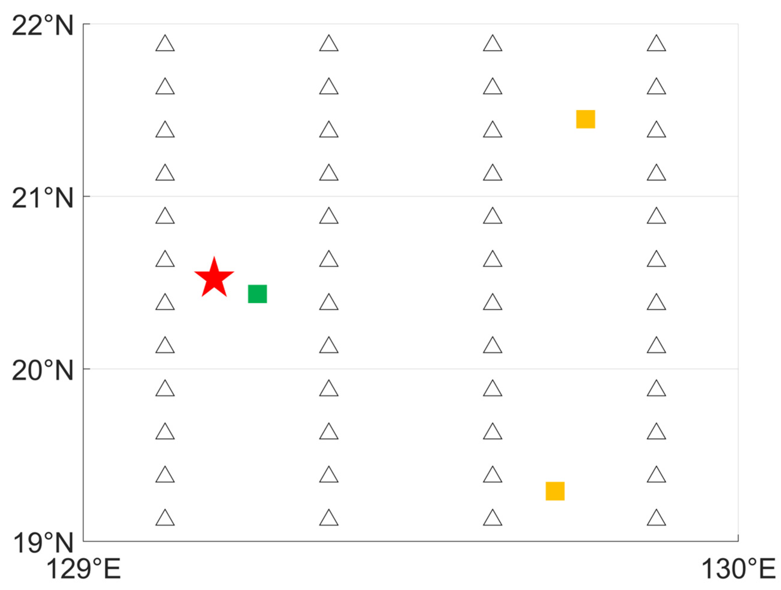
To verify the effectiveness of the method proposed in this paper, the northwest Pacific Ocean (19°–22° N, 129°–130° E) was selected as the experimental survey area, which is a typical deep-sea survey area. The four historical measured SSP stations used in the experimental survey area originated from the real-time temperature–salinity data measured in December 2022 and 2023, provided by the China Argo Real-time Data Center (http://www.argo.org.cn, accessed on 10 March 2025). Therefore, to better reduce the inversion errors of SSPs caused by different times and seasons, the quarterly average data of the WOA23 temperature–salinity model for the fourth quarter were chosen for analysis, with a spatial resolution of 0.25° × 0.25°, covering a total of 48 SSP stations. The sound-speed value at the shallowest depth of the historical measured SSPs was used as the surface sound speed for the multibeam, and one of the stations was randomly selected as the station for the inverted SSP. The SSP stations in the experimental survey area are shown in Figure 2.

Since the 1950s, ocean scientists have successively proposed empirical formulas to calculate sound speed that are applicable to different depth ranges for calculating SSPs [24]. At present, internationally recognized and more accurate empirical sound-speed formulas include the Wilson, Chen–Millero, and Del Grosso formulas. Lu et al. [25] have shown that the Chen–Millero formula has stronger applicability, and the National Oceanic and Atmospheric Administration (NOAA) of the United States also recommend using the Chen–Millero formula to calculate sound speed. Therefore, this paper uses this formula to calculate sound speed, as follows:

$$v=C_W(t,p)+A(t,p)S+B(t,p)S^{3/2}+D(t,p)S^2$$

(11)

where v is the sound speed in meters per second (m/s), t is the temperature in degrees Celsius (°C), S is the salinity, p is the pressure, and the specific calculation of the coefficients $C_W(t,p)$, $A(t,p)$, $B(t,p)$, and $D(t,p)$ can be found in the literature [25]. The applicable ranges of Equation (11) are a temperature scale of [0, 40] °C, a salinity scale of [5, 40]‰, and a seawater pressure scale of [0, 1000] bar.

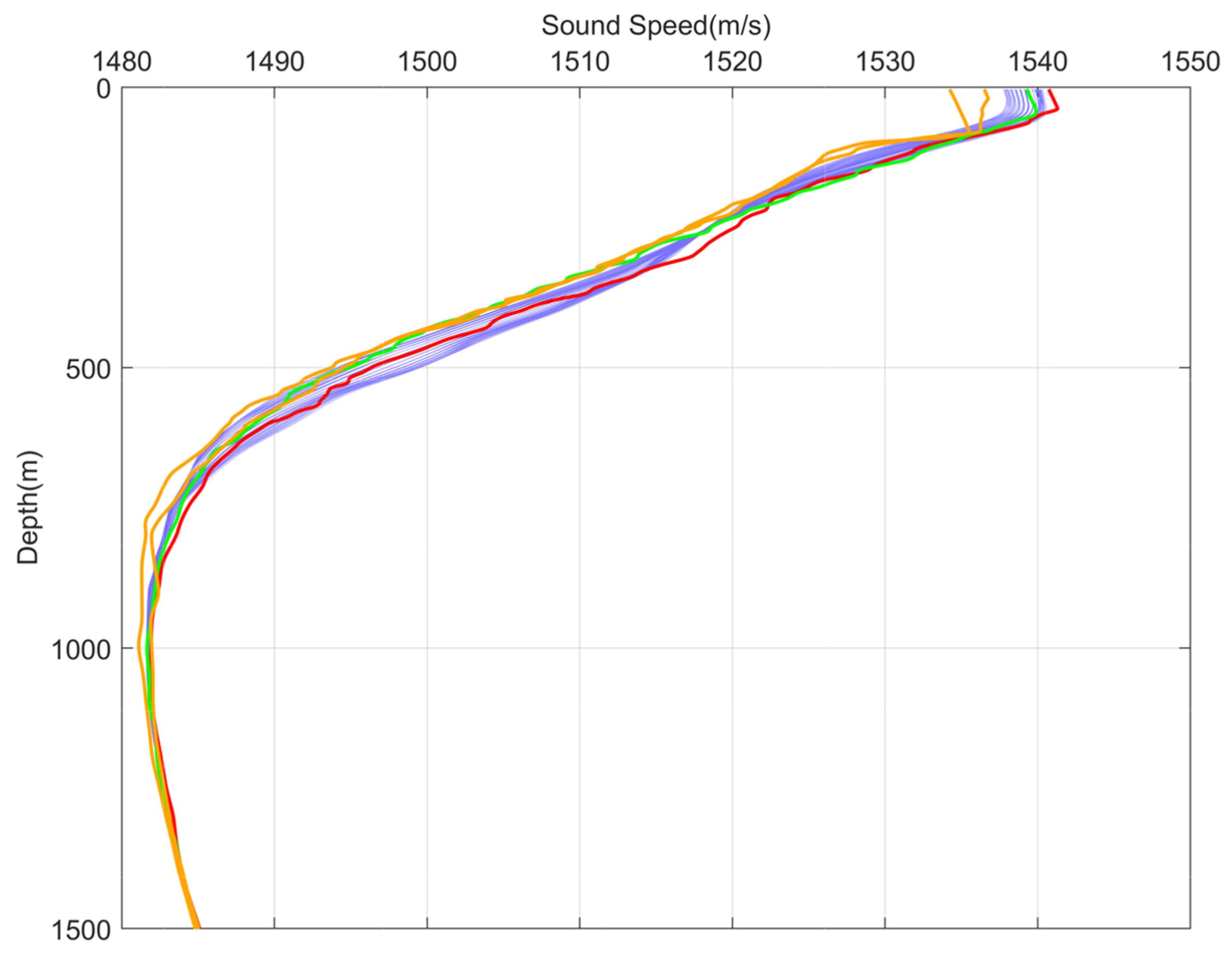
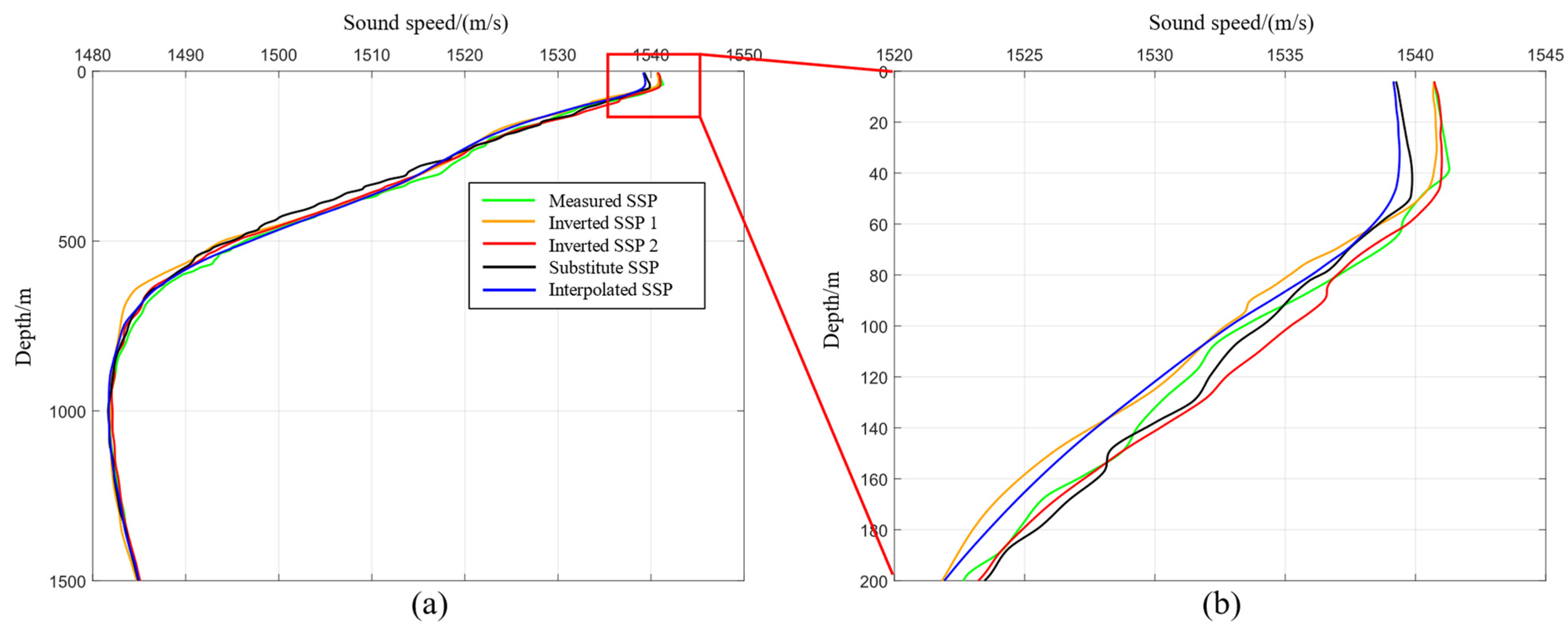
The analysis of the data from each measured SSP station indicates that the sampling depth is around 1500 m. Given that the sampling intervals of the measured SSPs are not fixed and differ significantly from those of the WOA23 SSPs, to facilitate the research, all SSPs in the survey area were standardized. Therefore, in this study, the Akima interpolation method was used to interpolate all SSPs in the survey area at 1 m intervals within the range of [0, 1500] m. The SSPs of each station in the survey area after interpolation are shown in Figure 3. It can be seen from the figure that the SSPs calculated by the WOA23 model are similar in structure to the measured profiles, with sound velocities ranging from 1480 to 1545 m/s. In the surface thermocline region, sound-speed changes are complex due to the influence of the marine environment, while the sound-speed structure below the sound channel axis is relatively stable, consistent with the typical variation characteristics of deep-sea SSPs.

As can be seen from Figure 3, the SSPs at the WOA23 model stations exhibit relatively gentle overall variations, with minimal differences among profiles at distinct locations within the survey area. In contrast, the measured SSPs show more pronounced changes in the shallow water zone due to the influence of seasonal climate, with the maximum variation in surface sound speed exceeding 5 m/s. The overall sound-speed structure differs significantly in the upper 1000 m of water depth, and the profiles display a sawtooth pattern rather than a smooth trend. Therefore, the SSPs measured in real-time are more complex than those predicted by the WOA23 model, necessitating further correction of the predicted profiles for high-precision multibeam depth measurement.

3.2. Experimental Process

In order to verify the rationality of this method, a deep-sea area with a water depth of about 1500 m was selected for the experiment. The measurement of high-precision SSPs was carried out with the aim of obtaining high-precision multibeam depth measurement data. Through the analysis of the errors of SSPs inverted through different methods, it was found that the SSP obtained by Inversion Method 2 was not much different from that obtained by the interpolation method. Therefore, to further verify the impact of the inverted SSPs on multibeam depth data, a deep-sea multibeam simulation with a beam angle of 1° and a beam opening angle of 120° was used to analyze the effect of the inverted SSPs on multibeam data sound-speed correction in a deep-sea area with a water depth of about 1500 m. The experimental process was as follows:

(1) EOF analysis: The SSP matrix of the measuring area was composed of the 51 standardized sound-speed profiles discussed in Section 3.1. After obtaining the SSP matrix in the survey area, an EOF analysis was conducted on the profiles following the steps outlined in Section 2.3.

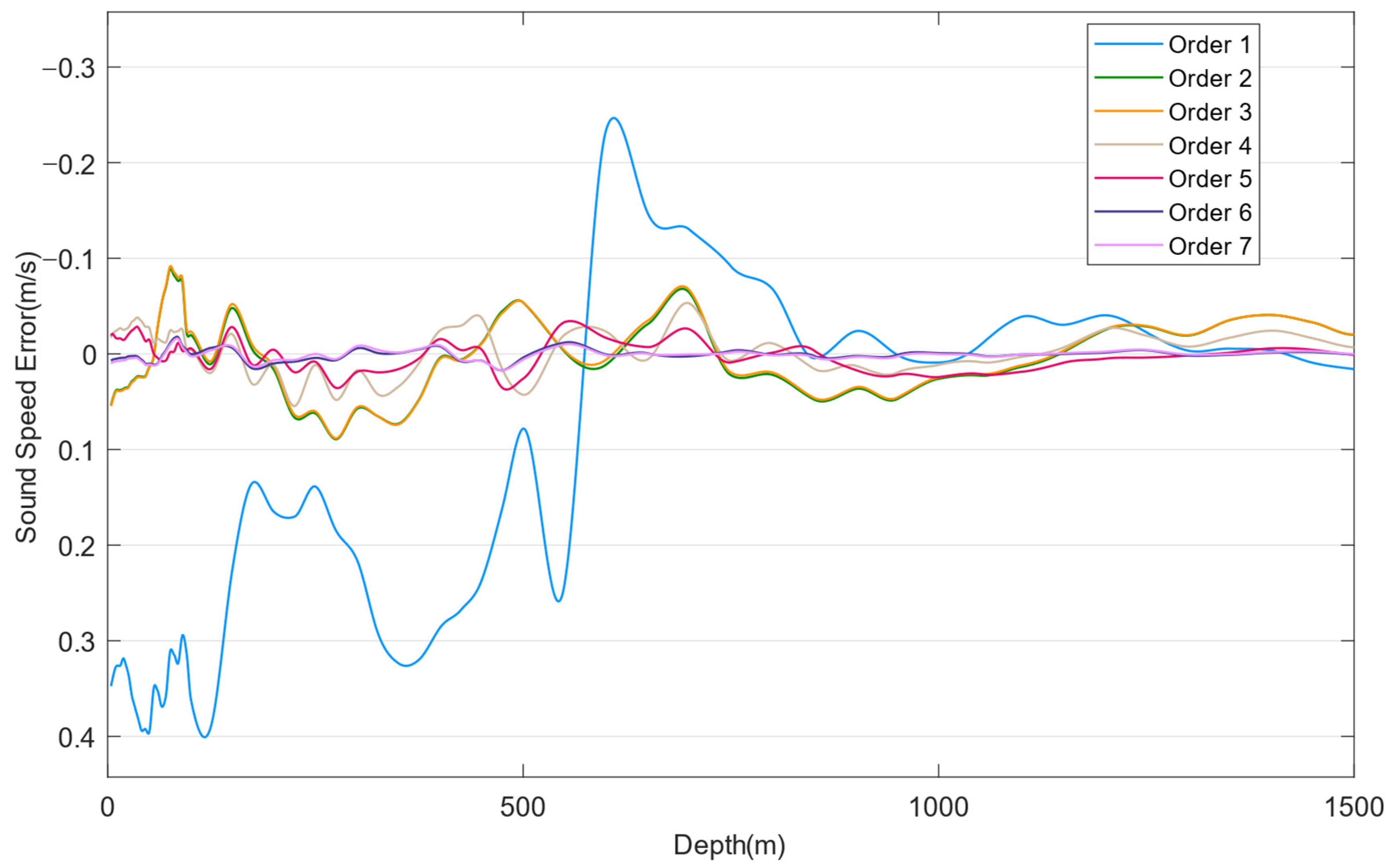
(2) Determination of EOF coefficient k: In order to reduce the order of time coefficients involved in the inversion of sound-speed profile and improve the efficiency of sound-speed profile inversion, the appropriate order k was determined by analyzing the variance contribution rate of the first seven orders of the EOF and the error of the reconstruction of sound-speed profile. The cumulative variance contribution rates of the first seven EOF modes are listed in

Table 1. Variance contribution rate of different EOF orders.

EOF Order	Variance Contribution Rate/%	Cumulative Variance Contribution Rate/%
1	98.372	98.372
2	99.259	0.888
3	99.867	0.608
4	99.938	0.069
5	99.984	0.047
6	99.992	0.008
7	99.997	0.005

, while the errors of the reconstructed SSPs are plotted in Figure 4.

As shown in Figure 4, the difference between the sound-speed profile represented by only the first EOF mode and the real sound-speed profile is relatively large in the upper 1000 m of water depth, with a maximum sound-speed difference of 0.4 m/s. In contrast, the maximum difference between the sound-speed profiles represented by the first three EOF modes and the real sound-speed profile is only 0.1 m/s. The differences between the sound-speed profiles represented by the first six and seven EOF modes and the real sound-speed profile are both within 0.02 m/s, and the error curves of the two reconstructed sound velocities are smoother, with smaller errors than those represented by the first five EOF modes. This indicates that as the number of EOF modes increases, the reconstructed sound-speed profiles more closely represent the real sound-speed profiles. Moreover, with increasing depth, the reconstructed sound-speed profiles using the EOF analysis are a very close match to the actual sound-speed profiles, with errors of less than 0.01 m/s. Therefore, to reduce the number of parameters and improve computational efficiency, the first six EOF modes were chosen to reconstruct the sound-speed profiles for inversion.

(3) Determination of the ALA optimization parameters: The search range of the upper and lower bounds of ALA is determined by the maximum and minimum values of the first six EOF time coefficients to determine the results, as shown in

Table 2. First six EOF coefficients and search range.

Coefficient	Maximum Value	Minimum Value
A1	89.96	−76.27
A2	29.82	−60.58
A3	39.34	−19.46
A4	34.49	−23.61
A5	15.35	−18.75
A6	16.10	−12.75

, in order to reduce the search space and improve the computational efficiency of the algorithm. It should be noted that when the optimal time coefficient is the search boundary, the optimal time coefficient should be searched again by expanding the search scope.

According to the content in process (2) of Section 3.2, the problem dimension was set to 6, representing the order of time coefficients involved in the inversion of the sound-speed profile, the population size was set to 20, the maximum number of iterations was set to 200, and the fitness function was the difference between the surface sound-speed measured by the multibeam sounding system and the inversion sound-speed profile. After the parameters were set, the process in Section 2.3 was followed for iterative optimization.

(4) Reconstruction and inversion of SSP: According to Equation (8), the sound-speed profile of the measurement area to be inverted is obtained.

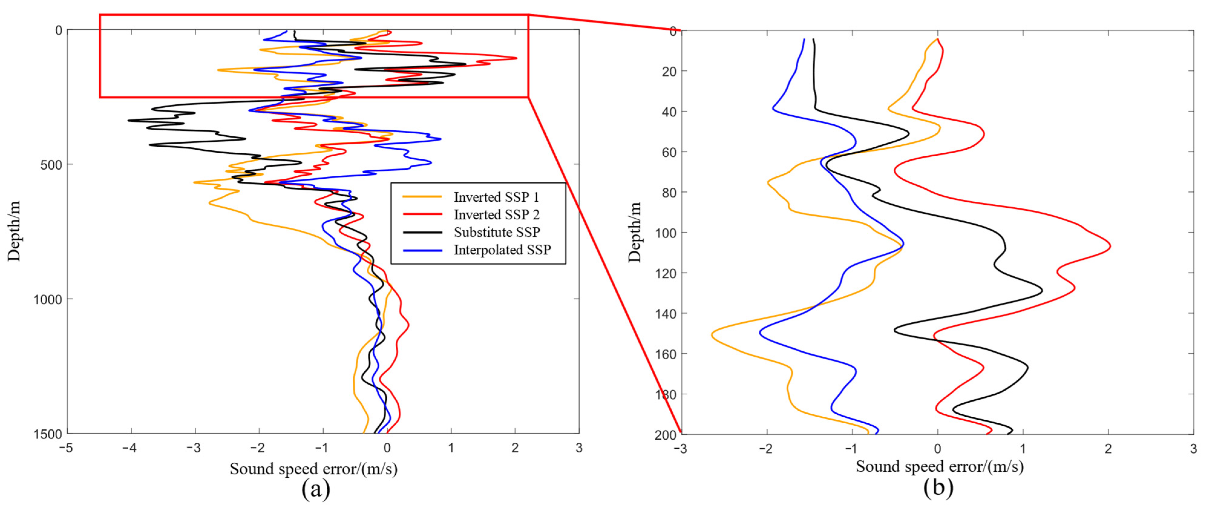
(5) Effectiveness verification: To verify the effectiveness of the method proposed in this paper, four methods were designed for comparative analysis; namely, the substitution method, the interpolation method, an inversion method combining WOA23 temperature–salinity model data with measured surface sound speed (named Inversion Method 1), and an inversion method combining WOA23 temperature–salinity model data and historical measured SSPs with measured surface sound speed (named Inversion Method 2). The substitution method is a commonly used method in current sound-speed correction by surveyors, which uses a nearby measured SSP as a substitute when the survey area lacks SSPs, causing terrain distortion, and then performs multibeam depth measurement data sound-speed correction. The interpolation method obtains the SSP at the missing location via spatial interpolation based on the spatial distribution of historical SSPs in the survey area, using the WOA23 model data as the historical SSP in the unfamiliar survey area and obtaining the SSP at the location to be inverted using the inverse distance-weighted interpolation method. Inversion Method 1 uses the WOA23 temperature–salinity model data in the survey area and inverts the SSP using ALA optimization based on the available surface sound-speed information. Inversion Method 2 uses the WOA23 temperature–salinity model data and a small amount of historical measured SSPs in the survey area, and inverts the SSP using the improved ALA optimization based on the available surface sound-speed information. Inversion Method 1 only used the WOA23 model data to verify the inversion of SSPs in the case where there were no historical SSP data in the unfamiliar deep-sea area for unmanned boats. The inversion process of Inversion Method 2 is essentially consistent with that of Inversion Method 1, and the only difference between the two methods is the different SSPs used.

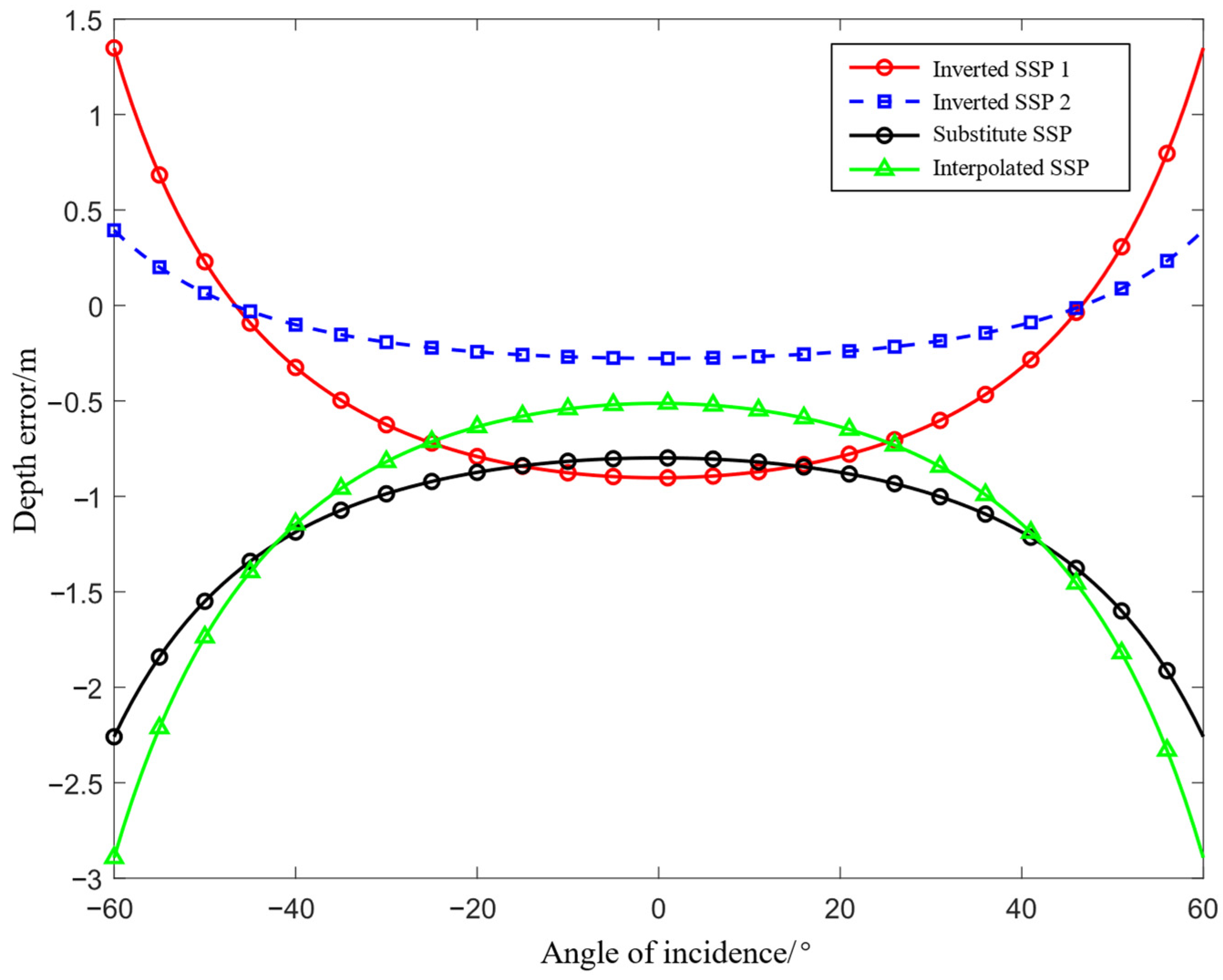
(6) Analysis of water depth error in the inversion of the sound-speed profile: According to the principle of constant gradient acoustic line-tracking, the multibeam echo time of the experimental water depth is obtained using the real sound-speed profile. The sound-speed profiles obtained by the four methods are followed by the constant gradient acoustic line-tracking according to the time, and the multibeam water depth-correction results of the different methods are obtained.

3.3. Evaluation Indicators

In order to comprehensively evaluate the reconstruction performance of each method, the RMSE (root mean square error), MAE (mean absolute error), and ME (maximum error) were selected as evaluation indexes. The RMSE measures the size of the reconstruction error; that is, the difference between the reconstructed value and the true value. The smaller the RMSE, the better the consistency between the reconstructed value and the true value. This index is sensitive to large errors and can effectively reflect the ability of the model to handle outliers or extreme values. The MAE quantifies the average difference between the reconstructed value and the true value. While it is less sensitive than the RMSE, it provides more intuitive results, with smaller values indicating better model performance. The ME identifies the worst-case prediction by measuring the largest absolute deviation between the reconstructed and true values, which is critical for applications requiring strict error control. The calculation formula is as follows:

$$\mathrm{RMSE}=\sqrt{{\displaystyle \frac{1}{m}}{\displaystyle \sum _{i=1}^m{\left({\widehat{x}}_i-x_i\right)}^2}}$$

(12)

$$\mathrm{MAE}={\displaystyle \frac{1}{m}}{\displaystyle \sum _{i=1}^m\left|{\widehat{x}}_i-x_i\right|}$$

(13)

$$\mathrm{ME}=\underset{1\le i\le m}{\max }\left|{\widehat{x}}_i-x_i\right|$$

(14)

where $x_i$ represents the sound-speed value at depth i in the measured SSP, ${\widehat{x}}_i$ represents the sound-speed value at depth i in the reconstructed SSP, and m represents the number of sound-speed points.

4. Results and Discussion

4.1. Sound-Speed Error Analysis of Inverted Sound-Speed Profile and Measured Sound Speed Profile

According to the experimental process in Section 3.2, the sound-speed error results of four different inversion methods are shown in Figure 5.

Figure 5a shows that the SSP structures inverted by the four methods are generally similar to the real SSPs. With the increase in water depth, the sound speed first increases and then decreases, reaching the minimum value at around 1000 m of water depth; thereafter, it continuously increases with the increase in water depth. Figure 5b provides a local enlargement of the SSPs in the range of [0, 200] m of water depth. The analysis shows that the SSPs obtained by the substitution method and the interpolation method significantly differ from the real SSPs in the shallow water area of [0, 50] m. In contrast, the SSPs obtained by Inversion Method 1 and Inversion Method 2, which incorporate surface sound speed as an inversion control index, have smaller differences from the real SSPs in the shallow water area.

The sound-speed errors of the SSPs inverted by the four methods are shown in Figure 6. To better compare the differences in the SSPs inverted by the four methods, in this study, we systematically evaluated the performance differences in the four sound-speed correction methods on the inverted SSPs based on three core indicators, namely, the MAE, ME, and RMSE, as presented in

Table 3. SSP errors of different methods.

Sound-Speed Correction Method	MAE (m/s)	ME (m/s)	RMSE (m/s)
Inversion Method 1	0.916	3.023	1.244
Inversion Method 2	0.531	2.051	0.745
Substitution Method	0.908	4.050	1.380
Interpolation Method	0.605	2.162	0.804

.

As can be seen from Figure 6 and Table 3, the surface sound-speed errors of the substitution method and the interpolation method were around 1.5 m/s, while the surface sound-speed errors of Inversion Method 1 and Inversion Method 2 were close to 0. The statistical results of ME, MAE, and RMSE show that Inversion Method 2 showed the best overall performance, with its MAE (0.531 m/s), RMSE (0.745 m/s), and ME (2.051 m/s) all being significantly lower than those of the other methods. Compared with the second-best method (interpolation method), its MAE was reduced by 12.3%, namely, from 0.605 to 0.531 m/s, and its RMSE was reduced by 7.4%, namely, from 0.804 to 0.745 m/s, which verifies its ability to resist interference in complex sound-speed fields. The stability defect of the substitution method is prominent: its ME is as high as 4.050 m/s, 1.97 times that of Inversion Method 2, indicating its high sensitivity to sudden changes in sound speed or noise interference. The significant difference between RMSE (1.380 m/s) and MAE (0.908 m/s) is about 0.472 m/s, which further reflects the strong dispersion of its error distribution. At the same time, there is a clear difference in the application scenarios of Inversion Method 1 and the interpolation method: compared with the interpolation method, Inversion Method 1 had a higher MAE (0.916 m/s) and RMSE (1.244 m/s), but its ME (3.023 m/s) was lower than that of the substitution method, and therefore it is suitable for scenarios with a higher tolerance for ME and those requiring quick calculations. Moreover, the interpolation method performed better than Inversion Method 1 in terms of MAE (0.605 m/s) and RMSE (0.804 m/s), but its ME (2.162 m/s) revealed its limitations in areas with complex sound-speed changes. The results of Inversion Method 2 show a significant improvement compared to the other three methods. Compared with the substitution method commonly used by surveyors, it improved by about 41.5%, 49.4%, and 46.0% in terms of MAE, ME, and RMSE, respectively. This indicates that the method significantly improved in the accuracy, stability, and reliability of SSP measurements, verifying the rationality of its theoretical model and proving that it can be a good alternative method for obtaining SSPs to ensure the quality of multibeam measurements when it is difficult to obtain real measurements of SSPs in deep-sea surveys. In conclusion, the SSP inversion method proposed in this paper provides a real and reliable SSP. When it is difficult to obtain real-time SSPs, it can provide reliable SSPs for the survey vessels in this area.

4.2. Depth Error Analysis of Inverted Sound-Speed Profile and Measured Sound-Speed Profile

The results and evaluation of the seafloor topography correction are shown in Figure 7 and

Table 4. Depth error of different methods.

Sound-Speed Correction Method	MAE/m	ME/m	RMSE/m
Inversion Method 1	0.634	1.349	0.701
Inversion Method 2	0.193	0.394	0.213
Substitution Method	1.146	2.259	1.216
Interpolation Method	1.086	2.893	1.264

.

Figure 7 and Table 4 demonstrate that the performance of the four methods in correcting the multibeam sound speed shows significant differences. Generally, the sound-speed errors are smaller for the central beams and larger for the edge beams. As the beam incidence angle increases, the water-depth error continuously grows. Inversion Method 2 demonstrates a significantly better error control capability than the other methods, indicating higher stability and interference resistance in SSP modeling. Its MAE (0.193 m), RMSE (0.213 m), and ME (0.394 m) are the lowest, reduced by 83.2%, 82.6%, and 82.5%, respectively, compared with the substitution method. The substitution and interpolation methods have clear limitations: although the interpolation method has a slightly better MAE (1.086 m) than the substitution method, its ME is as high as 2.893 m, the highest among all methods, indicating that it may cause serious distortion in areas with extreme gradient changes in the SSP. The performance of Inversion Method 1 is in the middle. Its MAE (0.634 m) and RMSE (0.701 m) are about 3.3 times that of Inversion Method 2, but its ME (1.349 m) is still within an acceptable range, suitable for situations where real-time SSPs cannot be obtained in the survey area and there are no historical SSPs. The substitution and interpolation methods need to avoid areas with strong thermoclines or significant noise interference, or improve their applicability by integrating other temperature–salinity data. Therefore, the SSP obtained by Inversion Method 2 can effectively correct the multibeam depth measurement data of deep-sea unmanned boat multibeam measurements, improving the efficiency and accuracy of the measurements.

4.3. Sound-Speed Correction Results of Multibeam Measured Bathymetric Data

To verify the actual application effect of the method proposed in this paper on deep-sea measurements, historical multibeam data from a certain area in the northwest Pacific Ocean were selected for validation and analysis. Raw survey line files were imported and processed in CARIS HIPS and SIPS software (version 6.1). The results are shown in Figure 8. Figure 8a shows the multibeam bathymetric point data in 2D view and Figure 8b shows the multibeam bathymetric point data in 3D view.

From Figure 8a,b, it is evident that the original multibeam data are severely distorted in the area shown due to sound-speed errors, especially at the edges. This is the typical “smiley face” phenomenon caused by sound-speed errors. It shows that the current sound-speed profile cannot effectively correct the original multibeam data, resulting in significant topographic deviations. The sound speed in the multibeam data needs to be corrected to eliminate these errors. As can be seen from Figure 8, the water depth of the central beam of the multibeam before and after the sound-speed correction is about 4850 m. The difference is not large, and this does not affect the surveyors’ assessment of the seabed topography. The depth of the edge beam increased from 4638 m (uncorrected) to 4914 m after correcting the measured sound speed, and the depth error reached 276 m, accounting for 5.6% of the actual depth. This value exceeds the 2022 edition of the Chinese National Standard for Hydrographic Surveys’ specification of a maximum depth error of no more than 2% of the measured depth. It can also be seen from the figure that the seabed topography is clearly distorted, which greatly affects the surveyors’ assessment of the seabed topography and reduces the credibility of the measured water depth data. After correcting the multibeam data of the sound-speed profile retrieved in this study, the water-depth value is 4881 m. Compared with the real water depth of 4914 m, the water-depth error is 33 m, accounting for about 0.7% of the actual water-depth value, which is less than 2%, thus meeting the requirements. The corrected seabed topography is essentially consistent with the real seabed topography, which does not affect the surveyors’ assessment of the seabed topography and improves the quality of the bathymetric data.

Figure 8 shows that the central beam’s depth error is only about 5 m, while the edge beam’s maximum error is around 276 m. This confirms the simulation results in Section 4.2 (see Figure 7). The central beam has a smaller error than the edge beam, and depth errors increase with beam angle. This further proves the effectiveness and practicality of our method.

5. Conclusions

In this study, we addressed the challenge of obtaining real-time SSPs in deep-sea multibeam bathymetry by proposing a novel joint inversion method that integrates WOA23 temperature–salinity model data, historical measured SSPs, and surface sound speed. Experimental validation in the northwest Pacific Ocean demonstrated the proposed method’s effectiveness and superiority. By combining WOA23 quarterly averaged data with historical measured SSPs, a high-resolution regional sound-speed field matrix was constructed, effectively suppressing interference due to seasonal and spatial heterogeneity. The experimental results showed that Inversion Method 2 reduced the MAE, RMSE, and ME of SSP reconstruction by 41.5%, 46.0%, and 49.4%, respectively, compared to traditional substitution methods, validating its robustness in complex sound-speed fields. When applied to multibeam bathymetric correction in deep-sea areas (approximately 1500 m water depth), Inversion Method 2 reduced the depth errors to 0.193 m (MAE), 0.213 m (RMSE), and 0.394 m (ME), achieving an over 82% error reduction compared to traditional substitution methods. This approach significantly mitigates the “smiley face” distortion caused by abrupt sound-speed gradients in edge beams, maintaining depth errors within the specification limit and improving the credibility of seabed topography data. By dynamically selecting the first six principal components of EOF (cumulative variance contribution rate >99.99%), computational complexity was reduced while ensuring reconstruction accuracy. ALA achieved an efficient global optimization of EOF coefficients through adaptive step size adjustment and composite differential operations, addressing the limitations of traditional genetic algorithms prone to local optima. This method provides a reliable solution for sound-speed correction in deep-sea regions lacking real-time SSP measurements and is particularly suitable for constrained platforms such as unmanned surface vehicles. However, the current approach relies on the spatiotemporal consistency of WOA23 and historical data. Future work should further validate its applicability in extreme marine environments (e.g., strong thermoclines and high-noise regions) and explore the deeper integration of machine learning and data assimilation techniques to enhance model generalization.

The proposed joint inversion method demonstrates significant technical advantages in deep-sea SSP reconstruction and multibeam bathymetric correction, offering theoretical support and practical tools for high-precision marine surveying. Future efforts will focus on algorithm parallelization and multi-source data fusion to expand its applications in global marine environmental monitoring.