Vortex-Induced Vibration Performance Prediction of Double-Deck Steel Truss Bridge Based on Improved Machine Learning Algorithm

Abstract

The span of a double-deck cross-sea bridge that can be used for both highway and railway purposes is usually 1 to 16 km. Compared with small-span bridges and single-layer main girder forms, its lightweight design and low damping characteristics make it more prone to vortex-induced vibration (VIV). To predict the VIV performance of a double-deck steel truss (DDST) girder with additional aerodynamic measures, the VIV response of a DDST bridge was investigated using wind tunnel tests and numerical simulation, a learning sample database was established with numerical simulation results, and a prediction model for the amplitude of the DDST girder and VIV parameters was established based on three machine learning algorithms. The optimization algorithm was selected using root mean square error (RMSE) and the coefficient of determination (R²) as evaluation indices and further improved with a genetic algorithm and particle swarm optimization. The results show that for the amplitude prediction of the main girder, the backpropagation neural network model is the most effective. The most improved algorithm yields an RMSE of 0.150 and an R² of 0.9898. For the prediction of VIV parameters, the Random Forest model is the most effective. The RMSE values of the improved optimal algorithm are 0.017, 0.026, and 0.295, and the R² values are 0.9421, 0.8875, and 0.9462. The prediction model is more efficient in terms of computational efficiency compared to the numerical simulation method.

1. Introduction

In the construction of cross-sea bridges, DDST bridges have become the preferred form of large-span bridges because of their ability to save line resources, their short construction period, and their excellent capacity—examples include the Pingtan Straits Rail-cum-Road Bridge [1] and the Xihoumen Rail-cum-Road Sea-Crossing Bridge [2]. In a wind field, after the incoming flow passes through the bridge’s main girder and other components, a part of the airflow separates to produce periodic shedding vortices. When the vortex shedding frequency is close to a certain order of the structure’s intrinsic frequency, it will trigger structural resonance, namely VIV [3,4]. Compared with small-span bridges and single-layer main girder forms, the DDST girder has more complicated aerodynamic properties and is prone to generating VIV at low wind speeds [5], which affects the durability of the bridge. Currently, the main tools for solving the VIV problem in bridges include wind tunnel testing and numerical simulations [6,7,8,9]. Wind tunnel testing is the most common method in VIV studies of bridge structures to study the aerodynamic performance, structural response, and flow field characteristics of objects by simulating wind speed and wind direction conditions found in the natural environment [10]. However, wind tunnel test studies are often economically expensive. Numerical simulation, based on fluid dynamics, simulates the interaction between fluids and structures through computer simulation. Although it is more convenient than wind tunnel testing, its computational cost is often quite expensive. Fang et al. [11] analyzed the frequency characteristics of the winding flow field near the cross-section of a DDST girder using numerical simulation and verified it via wind tunnel testing. Tang et al. [12] analyzed the vortex shedding performance of an optimized girder and discussed the corresponding aerodynamic mechanism using numerical simulation and wind tunnel tests.

Additional aerodynamic measures to control VIV in bridges are based on the principle of adding additional structures to change the aerodynamic profile of the main girder to improve its aerodynamic performance [13,14,15]. These additional structures include wind nozzles, deflector plates, and stabilizer plates. Zhan et al. [16] analyzed the VIV mechanism and control method for long-span bridges and found that modifying straight railings to wavy railings can effectively suppress vertical and torsional VIV. Yang et al. [17] analyzed the influence of a fully enclosed enclosure structure on the VIV performance of a DDST bridge using a combination of wind tunnel testing and a numerical calculation method.

Machine learning has powerful data analytics and is superior at handling high-dimensional, nonlinear problems [18,19]. Wei et al. [20] developed a deep reinforcement learning-driven autonomous learning framework, which has higher computational speed and accuracy in solving N–S equations. Yan et al. [21] developed a machine learning approach for rapidly estimating the VIV amplitude of a streamlined steel box girder during preliminary structural design. Li et al. [22] established a deep learning model to identify VIV forces on a main girder and verified its effectiveness through long-term monitoring of VIV on a large-span bridge.

There is still a gap in the current research on the prediction of the VIV response in large-span DDST girders. In view of the high cost, time consumption, and limited applicability of traditional analysis methods, this study aims to effectively and efficiently manage bridge VIV risks. Using the Huangjuetuo Bridge as the engineering background, wind tunnel testing, numerical simulation, and improved machine learning techniques are integrated in this research. First, the VIV response of the bridge is determined through a segmental model wind tunnel test. Second, numerical simulation is used to investigate the influence of changing the parameters of additional aerodynamic measures on the VIV of the DDST girder section. Finally, a prediction model based on an improved machine learning algorithm is developed to accurately predict the VIV response of the DDST girder section. This study provides a reference for research on the VIV response of large-span DDST bridges and serves as a useful supplement to traditional wind tunnel testing and numerical simulation research methods.

2. Vertical Bending VIV Response Analysis Method for Large-Span Bridge

2.1. Scanlan Nonlinear VIV Model

The Scanlan nonlinear VIV model describes the VIV force as a combination of the self-excited force induced by the motion of the structure and the self-excited force caused by vortex shedding [23]. The formula is expressed as follows:

$$f_{\mathrm{v}}={\displaystyle \frac{1}{2}}\rho U^2\left(2D\right)[Y_1\left(K\right)(1-∍{\displaystyle \frac{y^2}{D^2}}){\displaystyle \frac{y^{\prime }}{U}}+Y_2\left(K\right){\displaystyle \frac{y}{D}}+{\displaystyle \frac{1}{2}}{C}_{\mathrm{L}}\left(K\right)\sin (\omega t\left)\right]$$

(1)

where $f_{\mathrm{v}}$ is the vertical bend VIV force; $\rho$ is the air density; $U$ is the incoming wind speed; D is the girder height; $K$ is the vortex shedding reduction frequency; $Y_1\left(K\right)$ and $Y_2\left(K\right)$ are the aerodynamic stiffness terms as a function of $K$, determined experimentally; $∍$ is the degree of the nonlinear motion-induced effect as a function of $K$, determined experimentally; $y$ is the displacement over the transverse wind degree of freedom; $y^{\prime }$ is the velocity over the transverse wind degree of freedom; $C_{\mathrm{L}}\left(K\right)$ is the lift coefficient as a function of $K$, determined experimentally; $\omega$ means the vortex shedding frequency; and t means the time.

The vortex shedding frequency and its reduction frequency affect the magnitude of VIV force, which is the key link to analyzing the VIV of a large-span bridge. The aerodynamic profile of the section directly determines the flow and separation of the airflow after encountering the section, the frequency of vortex formation, and the drift speed. Therefore, adding additional aerodynamic measures to the bridge will directly change the aerodynamic profile of the main girder, which will affect the vortex shedding frequency and the VIV onset wind speed, locking interval length and the maximum VIV amplitude.

2.2. Realization of Vertical Bending VIV Response Analysis Method for Large-Span Bridge

The flow of analyzing the vertical bending VIV response of a large-span DDST bridge under additional aerodynamic measures by combining the wind tunnel testing and numerical simulation is shown in Figure 1, and the specific steps are as follows:

Step 1: Determine the onset wind speed, locking interval length, and maximum amplitude of the segment model through wind tunnel testing, and determine the wind attack angles of +3° and +5° for generating VIV. These two wind attack angles are used as the basis for further research.

Step 2: Determine a reasonable size of the computational domain according to the geometric dimensions of the main girder and perform meshing.

Step 3: Obtain the VIV force at each time step using the Ansys Fluent 2022R1 [24] solver combined with a user-defined function (UDF).

Step 4: Solve the vibration differential equations using the fourth-order Runge–Kutta method to obtain the velocity and displacement response at each time step.

Step 5: Based on the velocity and displacement response calculated in Step 5, update the grid node positions with the dynamic grid model and determine whether the computation stopping condition is met. If it is satisfied, stop the calculation condition; if not, carry out the calculation in the next time step. Cycle according to Steps 3–5 to realize the VIV response analysis of the main girder section.

3. Prediction of Vertical Bending VIV Performance of Large-Span Bridge Based on Improved Machine Learning Algorithm

3.1. Determination of Input Parameters

Parameters of additional aerodynamic measures can be identified as important variables affecting VIV performance. The main additional aerodynamic measures are the wind nozzle, deflector plate, and central stabilizer plate. Among them, the simulation working condition of the wind nozzle is set using the variable of wind nozzle angle–wind nozzle tip position–wind attack angle; the simulation working condition of the deflector plate is set using the variable of deflector plate position–deflector plate height ratio–wind attack angle; and the simulation working condition of the combined measures is set using the variable of wind nozzle or not–deflector plate or not–central stabilizer plate or not–wind attack angle. To predict the amplitude of the DDST girder section under different wind speeds, the wind attack angle, reduced wind speed, and additional aerodynamic measures are taken as feature inputs. The reduced amplitude of vertical bending is taken as the feature output. For the prediction of VIV of the DDST girder section under different additional aerodynamic measures, the wind attack angle and additional aerodynamic measure parameters are taken as the feature inputs, and the onset wind speed, the locking interval length, and the maximum reduction amplitude of VIV are taken as the feature outputs.

3.2. Three Machine Learning Algorithms and the Optimization Algorithm

The prediction ability of different machine learning algorithm models may differ for different problems [25]. Therefore, the VIV response of the DDST bridge is predicted using three common machine learning algorithms: SVR, BPNN, and RF. Performance evaluation indices select the optimal model, which is improved by combining GA and PSO.

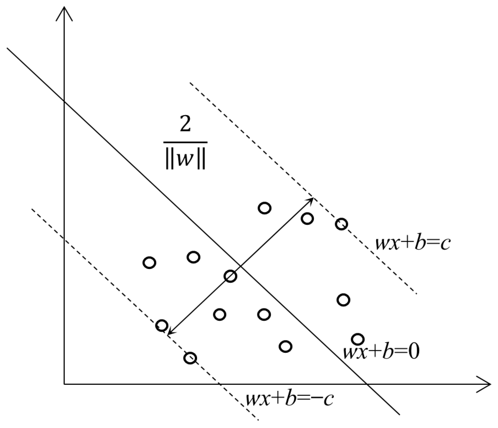
• Support Vector Regression Algorithm:

SVR [26] is a supervised learning algorithm. The regression model is obtained by using the kernel function to map the data into a high-dimensional space and finding the optimal hyperplane in that space to maximize the interval between the training data, as shown in Figure 2. Predicting the VIV response of the DDST bridge belongs to the typical regression problem, and the dataset is small, which meets the applicable conditions of SVR.

2.

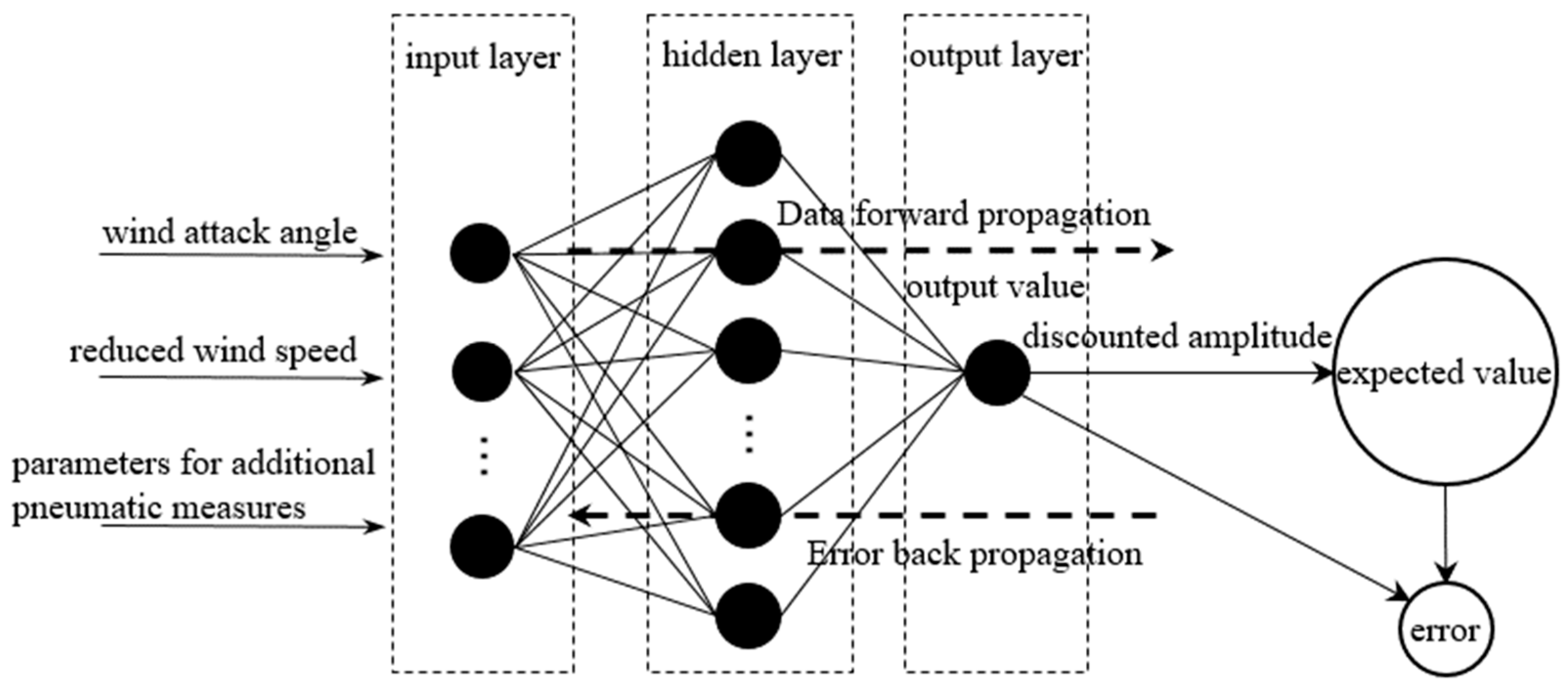
Backpropagation Neural Network Algorithm:

BPNN is a kind of artificial neural network, which has the advantage of being able to approximate any complex nonlinear function and is robust to noise and incomplete data [27,28]. As shown in Figure 3, BPNN is divided into two parts: forward propagation of data and backward propagation of error. Sigmoid and ReLU are used as activation functions in forward propagation. Its working principle is as follows: the input value is propagated forward from the input layer to the output layer through the hidden layer, and the output value is obtained; then, the error between the output value and the expected value is propagated backward through the hidden layer, and the weights in the model are adjusted continuously to reduce the error between the output value and the expected value. Therefore, using BPNN to analyze the VIV response data of the DDST girder is feasible. The parameters of the BPNN network are mainly the number of hidden layers and nodes in hidden layers. We use the Adam Optimizer to optimize BPNN. The learning rate is set to 0.01, the epoch is set to 100, and the model converges when we reach the 19th training epoch.

3.

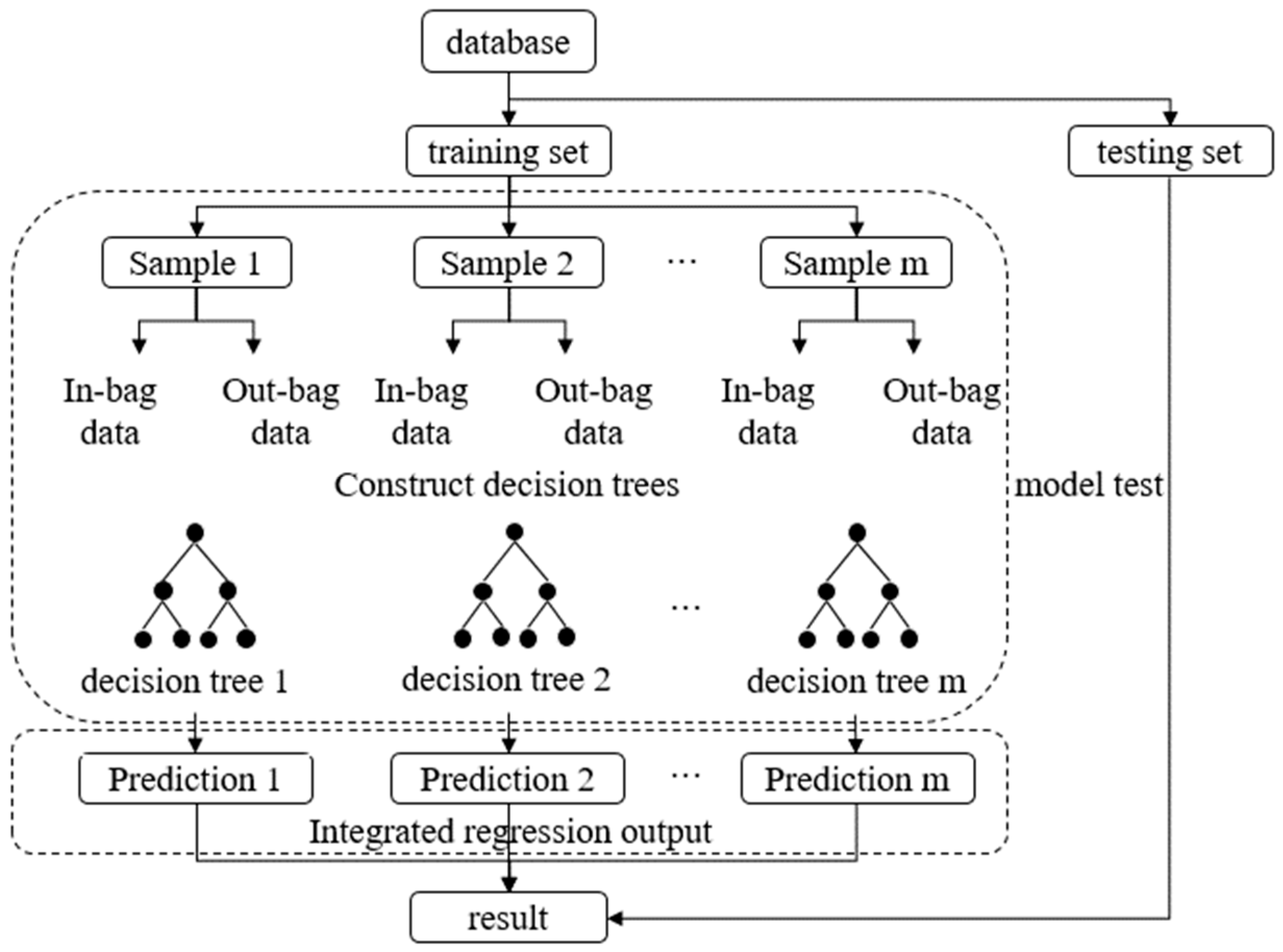
Random Forest Algorithm:

RF is an integrated learning method suitable for classification and regression. RF combines the advantages of decision trees and randomness, has strong data mining ability and high prediction accuracy, and, thus, is widely used to solve prediction class problems [29]. As shown in Figure 4, the use of Random Forest to deal with the regression problem is divided into two parts: One is to construct a decision tree from the training set and put back to randomly extract 2/3 of the samples (bag of data) as a sample set to train the decision tree, segmentation based on random features until the stopping conditions are met, and the remaining 1/3 of the samples (out-of-bag data) are used to evaluate the error, which can be used to obtain a single decision tree model, and a total of extracted and trained m times; then, m decision tree models can be obtained. Second is the integrated regression output, the prediction result of each decision tree, which is averaged as the final result output. The RF network parameters are the number of decision trees (n) and the minimum number of leaves (leaf).

4.

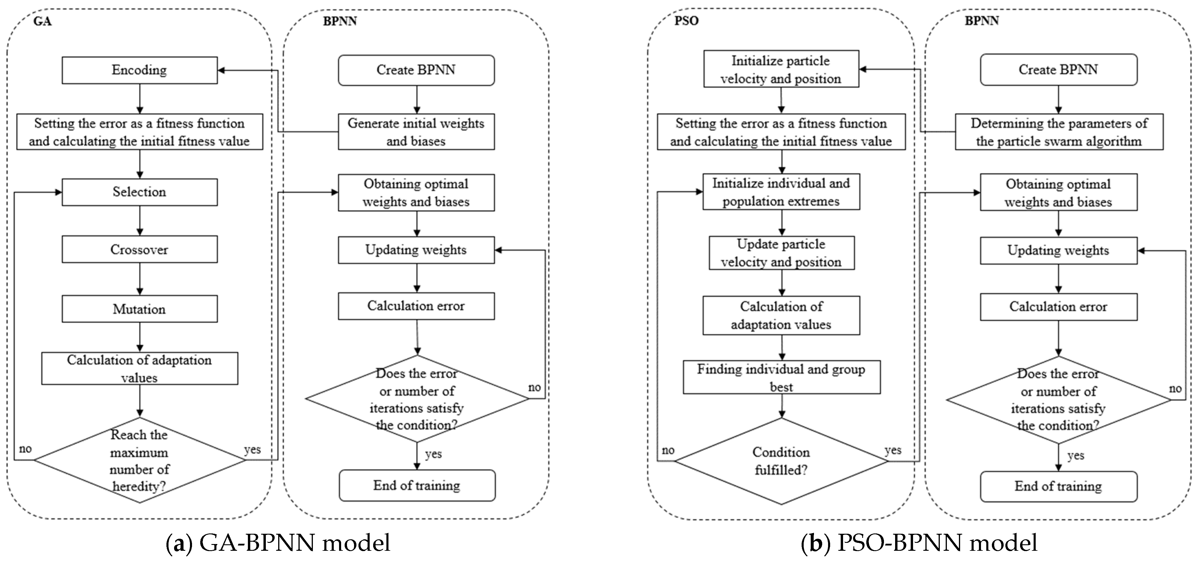
Genetic Algorithm:

As shown in Figure 5, GA is an optimization algorithm based on the principle of biological evolution. It simulates the genetic and evolutionary processes in nature and gradually searches and optimizes the solution of the problem by performing operations such as selection, crossover, and mutation on the individuals in the solution space [30,31].

5.

Particle Swarm Optimization:

PSO [32,33] is an optimization algorithm based on group intelligence. Its basic idea is to regard the problem’s solution space to be optimized as a swarm of particles in a multidimensional space. Each particle represents a candidate solution, and each particle has its own position and velocity. Each particle updates its own position and velocity according to its own experience and the experience of the group, the principle of which is shown in Figure 6.

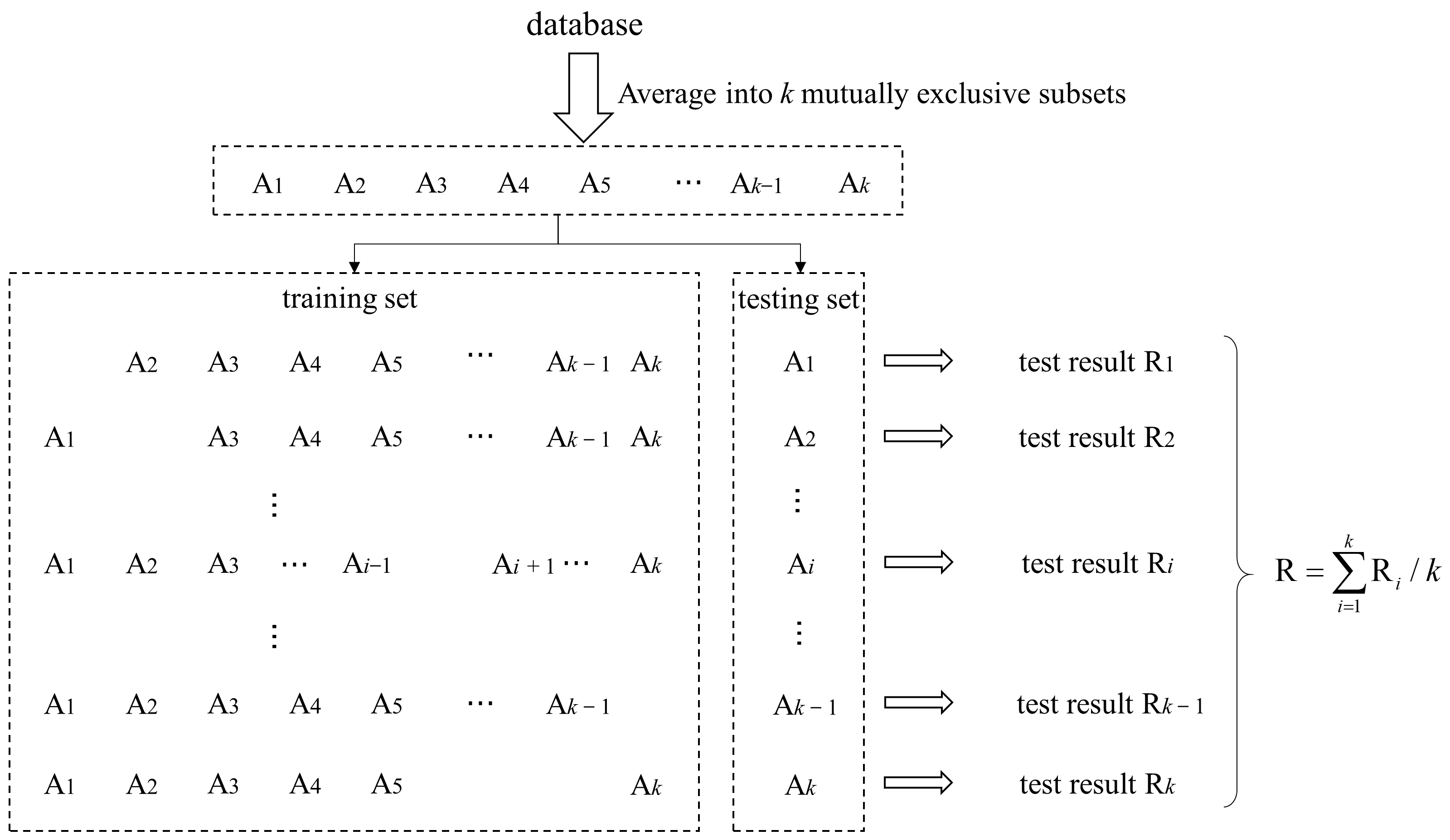
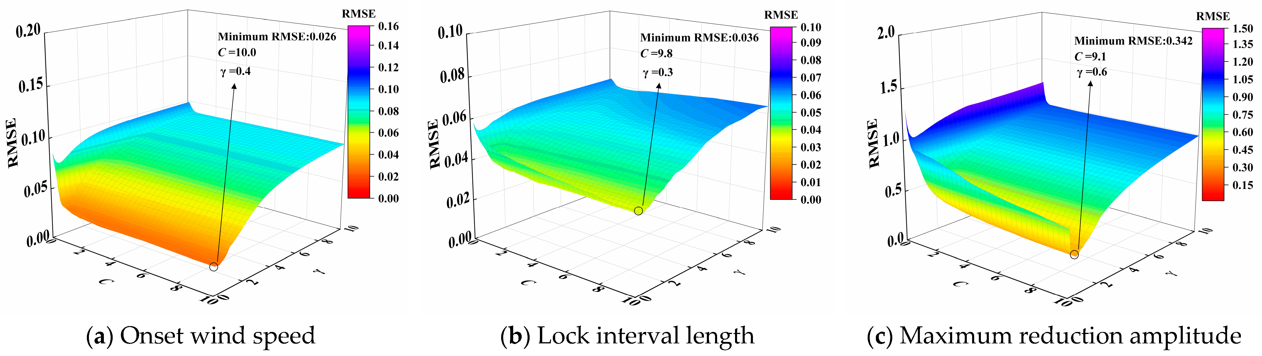
3.3. Performance Evaluation Methods and Parameter Optimization

The k-fold cross-validation enables data partitioning of machine learning models using a limited sample set. In the k-fold cross-validation method, the division of the sample set is to divide the original sample set into k subsets of approximately equal size evenly and without repetition according to the established rules. Each subset is independent, and in the subsequent verification process, one of the subsets will be used as the verification set, while the rest of the k-1 subsets will be combined to form the training set. This cycle is k times to ensure that each subset has the opportunity to act as the verification set and then comprehensively and objectively evaluate the performance of the model. The analysis path is given in Figure 7.

Optimization of the parameters in each model is performed through the training set, and the prediction ability of the three algorithms is evaluated using the test set. The prediction results are evaluated using the root mean square error (RMSE) and the coefficient of determination (R²). A monotonic inverse correlation exists between RMSE magnitude and model precision, where asymptotic convergence toward zero indicates error minimization. Its calculation formula is as follows:

$$\mathrm{RMSE}={\displaystyle \frac{1}{k}}{\displaystyle \sum _{j=1}^k\sqrt{\frac{1}{n}{\displaystyle \sum _{i=1}^n{\left(Y_i-y_i\right)}^2}}}$$

(2)

where k is the number of cross-validation folds, n is the number of samples, y_i and Y_i are the desired and predicted outputs, respectively.

The closer the R² is to 1, the higher the prediction accuracy of the model, which is calculated as follows:

$${\mathrm{R}}^2=1-{\displaystyle \sum _{i=1}^n{\left(y_i-\overline{Y_i}\right)}^2}/{\displaystyle \sum _{i=1}^n{\left(y_i-\overline{y}\right)}^2}$$

(3)

where $y_i$ is the model expected output, $\overline{Y_i}$ is the model predicted output, $\overline{y}$ is the test set mean, n means the number of samples.

3.4. VIV Response Prediction Model Based on Improved Machine Learning Algorithm

The VIV response analysis method is combined with three common algorithms to establish a prediction model, and the GA and PSO algorithms are further improved to achieve better prediction results. The modeling is shown in Figure 8, and the specific analysis steps are as follows:

Step 1: Numerical simulation can be used to obtain the onset wind speed, locking interval length, maximum reduction amplitude, and other data on the VIV of the large-span DDST bridge under additional aerodynamic measures to establish a sample set. The dataset for predicting the VIV characteristic parameters of the DDST girder section is defined as the VIV-R dataset, which includes the calculation results of 58 simulation conditions, including the original section. In a range of 1.7 m/s~3.0 m/s, 20 results of different wind speeds are taken for each working condition, and the VIV-A dataset containing 1160 samples can be obtained to predict the amplitude of the DDST girder section.

Step 2: Import the datasets VIV-R and VIV-A into Matlab R2022b [34] for normalization.

Step 3: Randomly divide the training set and test set according to the k-fold cross-validation method and train the three machine algorithm models through the training set to optimize their respective parameters.

Step 4: Based on the optimal parameter settings of each algorithm, the test set is used to evaluate the three models by combining the minimum RMSE and R². The optimal algorithm model is selected and further improved and optimized by combining the GA and PSO algorithms.

Step 5: The improved optimal algorithm model can be used to predict the VIV response parameters.

4. Engineering Example Analysis

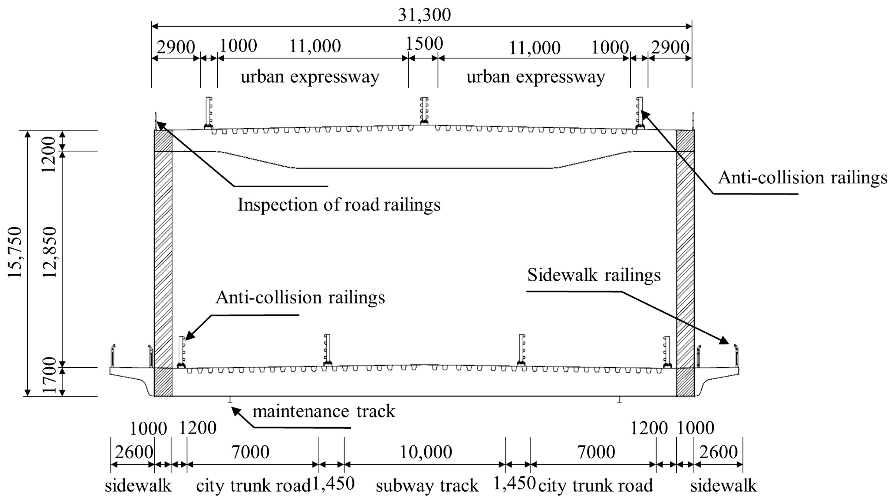
4.1. Engineering Background

Huangjuetuo Bridge is a large-span dual-purpose suspension bridge for expressways and railroads under construction in China. Except for the web members, the bridge cross-section is almost unchanged along the bridge axis’s direction, and the DDST girder’s standard cross-section is shown in Figure 9. The results of the calculation of structural dynamic characteristics for the bridge’s main modes are shown in

Table 1. Structural dynamic characteristics of the Huangjuetuo Bridge.

Model	Frequency	Mass	Moment of Inertia	Vibration Pattern
3	0.211 Hz	6.845 × 104 kg/m	/	first-order symmetric vertical bending
4	0.237 Hz	7.008 × 104 kg/m	/	first-order antisymmetric vertical bending
11	0.478 Hz	/	1.309 × 107 kg·m2/m	first-order symmetric torsion
25	0.706 Hz	/	1.228 × 107 kg·m2/m	first-order antisymmetric torsion

. These parameters will be used as an important basis for the design of a segmental model in the wind tunnel test.

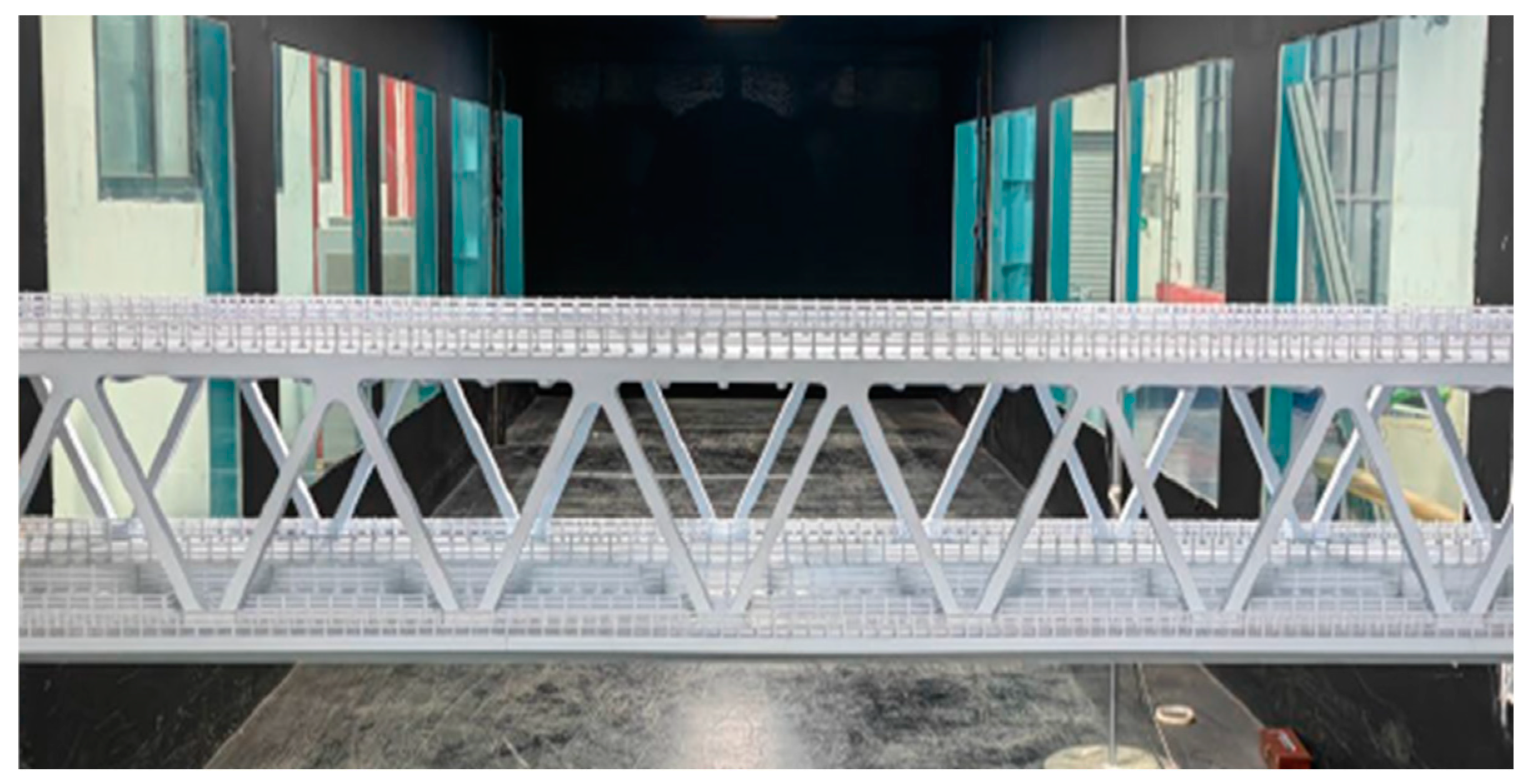
4.2. Segment Model VIV Test

The segmental model VIV test of the target bridge was carried out in the wind tunnel laboratory of Chongqing University. As shown in Figure 10, the model was scaled down to a ratio of 1:55, with the following model dimensions: longitudinal axis (2.20 m), transverse axis (0.569 m), and vertical axis (0.286 m). The segmental model was mounted with a spring-suspension system in the wind tunnel test, and the test wind speed ratio was 1:4.48. The main design parameters of the bridge model are shown in

Table 2. Main design parameters of the test model.

Parameter	Unit	Real Bridge Value	Similarity Ratio	Test Model Value
height	m	15.75	1:55	0.286
width	m	31.30	1:55	0.569
mass	kg/m	6.845 × 104	1:552	22.628
moment of inertia	kg·m2/m	1.309 × 107	1:554	1.431
radius of gyration	m	13.83	1:55	0.251
vertical bending frequency	Hz	0.211	-	2.218
torsion frequency	Hz	0.478	-	5.033
vertical bending damping ratio	%	0.50%	1:1	0.38%
torsion damping ratio	%	0.50%	1:1	0.31%

.

In the uniform flow field, the VIV measurement test is carried out on the DDST girder section under 0°, ±3°, ±5° wind attack angles, and the test wind speed is 0~10 m/s. The vertical amplitude is defined as A, the test wind speed is defined as U, and the test results are dimensionless. The reduced amplitude of the vertical bending VIV is taken as the ratio of the amplitude to the height of the model girder, i.e., y = A/D. The reduced wind speed is taken as the ratio of the test wind speed to the product of the base frequency of the vertical bending of the structure and the height of the model girder, i.e., $V_{\mathrm{r}}=U/f_{\mathrm{b}}D$, where $f_{\mathrm{b}}$ = 2.22 Hz. The test results are shown in Figure 11.

According to the test results, it can be seen that the segmental model undergoes significant vertical bending VIV at the +3° and +5° wind angles of attack. When vertical bending VIV occurs in the segment model at a +3° wind attack angle, the reduced wind speed in the locked interval ranges from 1.85 to 2.35, and the maximum reduced amplitude reaches 0.264 when the reduced wind speed is 2.12. When vertical bending VIV occurs at a +5° wind attack angle, the reduced wind speed in the locked interval ranges from 1.76 to 2.33, and the maximum reduced amplitude reaches 0.343 when the reduced wind speed is 2.14. When the wind attack angle increases from +3° to +5°, the locking interval length and the maximum reduction amplitude of the vertical bending VIV will increase, and the onset wind speed will advance.

4.3. Numerical Simulation Results of Additional Aerodynamic Measures for Two Wind Attack Angles

The numerical simulation parameters are set as follows: the flow is steady and incompressible, and the static force is treated as steady, without considering the influence of temperature. The corresponding mathematical model is the Reynolds time-averaged N-S equation, and the turbulence model is the SST k-ω model, which can adapt well to the bluff body section. The near wall is processed by the standard wall function. The coupled algorithm with better robustness is selected for the pressure velocity coupling solution method. The second-order upwind format is selected for the spatial discretization format. The turbulence intensity is 0.50%, and the calculation residual is controlled to 1 × 10⁻⁵. The calculation time is set to 10 s to ensure the complete convergence of the calculation. The time step is 1 × 10⁻⁴ s.

The calculation domain of CFD numerical simulation is divided into two parts: internal region and external region. The external region uses a structured grid, and the internal region uses an unstructured grid. Based on the actual width of the model, B = 0.569 m, the internal area size is 4B × 4B (width × height), and the external area size is 32B × 16B (width × height), as shown in Figure 12. The two-dimensional model of the double-deck steel truss girder section is arranged in the middle of the calculation domain, with an entrance distance of 8B, exit distance of 24B, and upper- and lower-boundary distances of 8B, respectively. The blocking rate of the model in the calculation domain is 0.5%, which is less than the allowable value of 5%, which can avoid the influence of the wake reflux.

Diagrams of external grid division and internal grid division are shown in Figure 13 and Figure 14.

The SST K-ω turbulence model selected requires the wall y+value to be less than 1, so the grid thickness near the wall of the first layer should be less than 9 × 10⁻⁵ B according to the set wind speed, dynamic viscosity, and air density. When dividing the internal grid, the double-layer steel truss girder section is divided into three parts: bridge deck, belly bar and railing. We set the maximum mesh size to 7 × 10⁻⁵ B. The maximum size of the near wall grid of the bridge deck and belly bar is set to 5 × 10⁻⁵ B, the linear growth rate is set to 1.1, and the boundary layer is set to 10 layers. Due to the small size of the railing part, the maximum size of the near wall grid is set as 2 × 10⁻⁵ B, and a 10-layer boundary layer with a linear growth rate of 1.1 is also set. The external structured grid size is set to 3 × 10⁻⁴ B. According to the above settings, the total number of 2D section model grids generated by ANSYS ICEM 2022R1 is about 784,000.

In the numerical simulation, we mainly consider the wind nozzle, deflector plate, and central stabilizer plate, as shown in Figure 15. Numerical simulation can obtain the relevant VIV data of the bridge under additional aerodynamic measure conditions, and we take 20 wind speed conditions each under the reduced wind speed of 1.7 m/s~3.0 m/s to be used to build the VIV-R and VIV-A datasets. The k-fold cross-validation method is also used to obtain the training and validation sets.

Before performing numerical simulation, its accuracy needs to be verified [35]. The UDF program is activated during the numerical simulation to simultaneously solve for the reduction amplitude of the vertical bending VIV in the DDST girder section, and the calculated results are compared with the wind tunnel test results, as shown in Figure 16.

As can be seen from Figure 16, the maximum reduction amplitude of the numerical simulation at the +3° wind attack angle is 0.298, and the error between the numerical simulation and the test is 12.9%. The maximum reduction amplitude of the numerical simulation at the +5° wind attack angle is 0.374, and the error between the numerical simulation and the test is 9.0%. The locking interval range, amplitude size, and change trend of vertical bending VIV obtained from numerical simulation are similar to the wind tunnel test results, which can be used for the calculation of the VIV response of the DDST girder section.

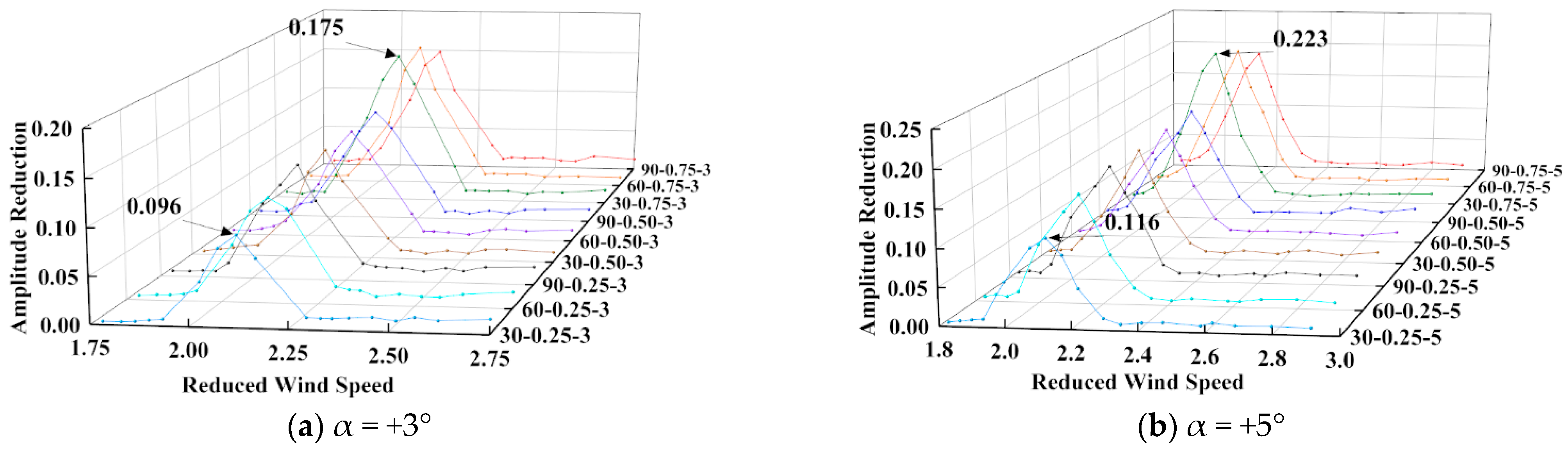
4.3.1. Vibration Suppression Rule for Wind Nozzle

Fix the wind nozzle position at the top chord when setting up the wind nozzle simulation condition. The wind nozzle tip position is defined as the ratio between the distance from the wind nozzle tip to the upper edge of the wind nozzle (h) and the wind nozzle height (D). A schematic diagram of the wind nozzle is shown in Figure 17.

With the angle of the wind nozzle, the position of the wind nozzle tip, and the angle of attack as variables, 18 kinds of simulated conditions of the wind nozzle were set. The simulated working conditions are shown in

Table 3. Simulation working conditions for wind nozzle.

Condition Number *	Wind Nozzle Angle	Wind Nozzle Tip Position	Wind Attack Angle	Condition Number	Wind Nozzle Angle	Wind Nozzle Tip Position	Wind Attack Angle
SW30-0.25-3	30°	0.25	+3°	SW30-0.25-5	30°	0.25	+5°
SW30-0.50-3	30°	0.50	+3°	SW30-0.50-5	30°	0.50	+5°
SW30-0.75-3	30°	0.75	+3°	SW30-0.75-5	30°	0.75	+5°
SW60-0.25-3	60°	0.25	+3°	SW60-0.25-5	60°	0.25	+5°
SW60-0.50-3	60°	0.50	+3°	SW60-0.50-5	60°	0.50	+5°
SW60-0.75-3	60°	0.75	+3°	SW60-0.75-5	60°	0.75	+5°
SW90-0.25-3	90°	0.25	+3°	SW90-0.25-5	90°	0.25	+5°
SW90-0.50-3	90°	0.50	+3°	SW90-0.50-5	90°	0.50	+5°
SW90-0.75-3	90°	0.75	+3°	SW90-0.75-5	90°	0.75	+5°

* The first digit in the working condition number represents the wind nozzle angle; the second digit represents wind nozzle tip position; and the third digit represents the wind attack angle. For example, SW30-0.25-3 indicates that a wind nozzle with an angle of 30° and wind nozzle tip position of 0.25 is added, and the wind attack angle is +3°.

. The VIV response of the 18 nozzle simulated conditions is shown in Figure 18.

As can be seen from Figure 18, when h/D = 0.25 at the tip of the wind nozzle, the maximum reduction amplitude under the condition of 30° wind nozzle angle is the smallest, which is 0.096 at the +3° wind attack angle, decreasing 67.9% compared with the bridge section, and 0.116 at the +5° wind attack angle, decreasing 68.8% compared with the bridge section. When the tip of the wind nozzle h/D = 0.50, the maximum reduction amplitude of the nozzle angle is 30°, 60° and 90°. When the tip of the wind nozzle h/D = 0.75, the maximum reduction amplitude of the 90° wind nozzle angle is the smallest, which is 0.148 at the +3° wind attack angle, 50.4% less than the bridge section, and 0.182 at the +5° wind attack angle, which is 51.2% less than the bridge section. When the angle of the wind nozzle is constant, the maximum reduction amplitude of the DDST girder section increases with the increase in the wind nozzle tip position, and the change amplitude is the lowest. When the tip of the wind nozzle is 0.25 and the nozzle angle is 30°, the nozzle parameters are optimal, and the upper chord nozzle has the best effect on suppressing the VIV of the DDST girder section.

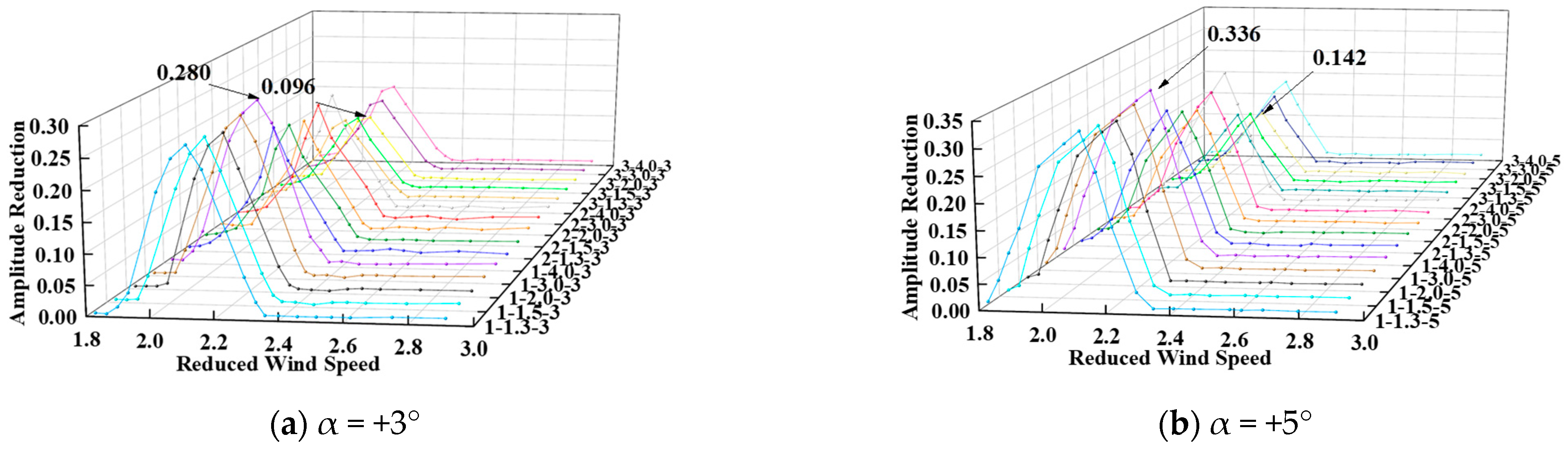
4.3.2. Vibration Suppression Rule for Deflector Plate

Fix the width of the deflector when setting up the deflector to simulate the working conditions. Define the deflector height ratio as the ratio of the height of the belly bar or the height of the lower chord bar to the deflector height. Taking the height ratio and position of the deflector as variables, 30 simulated working conditions of the deflector were set. The experimental parameters are illustrated in

Table 4. Simulation working conditions for deflector plate.

Condition Number *	Deflector Height Ratio	Wind Attack Angle	Condition Number	Deflector Height Ratio	Wind Attack Angle
SD1-1.3-3	1.3	+3°	SD1-1.3-5	1.3	+5°
SD1-1.5-3	1.5	+3°	SD1-1.5-5	1.5	+5°
SD1-2.0-3	2.0	+3°	SD1-2.0-5	2.0	+5°
SD1-3.0-3	3.0	+3°	SD1-3.0-5	3.0	+5°
SD1-4.0-3	4.0	+3°	SD1-4.0-5	4.0	+5°
SD2-1.3-3	1.3	+3°	SD2-1.3-5	1.3	+5°
SD2-1.5-3	1.5	+3°	SD2-1.5-5	1.5	+5°
SD2-2.0-3	2.0	+3°	SD2-2.0-5	2.0	+5°
SD2-3.0-3	3.0	+3°	SD2-3.0-5	3.0	+5°
SD2-4.0-3	4.0	+3°	SD2-4.0-5	4.0	+5°
SD3-1.3-3	1.3	+3°	SD3-1.3-5	1.3	+5°
SD3-1.5-3	1.5	+3°	SD3-1.5-5	1.5	+5°
SD3-2.0-3	2.0	+3°	SD3-2.0-5	2.0	+5°
SD3-3.0-3	3.0	+3°	SD3-3.0-5	3.0	+5°
SD3-4.0-3	4.0	+3°	SD3-4.0-5	4.0	+5°

* The first digit in the working condition number represents the additional position of the deflector, “1” represents the “belly bar”, “2” represents the “lower chord bar” and “3” represents the “belly bar + upper chord bar”; the second digit represents the height ratio of the deflector; and the third digit represents the wind attack angle. For example, “SD1-1.3-3” indicates that a deflector with a height ratio of 0.13 is added to the belly bar, and the wind attack angle is +3°.

. The size of the deflector in the table is the model size. The specific VIV response for the 30 deflector simulated conditions is shown in Figure 16.

As can be seen from Figure 19, when the height ratio of the deflector is less than 2, the maximum reduction amplitude gradually decreases with the increase in the height ratio; when the height ratio of the deflector is greater than 2, the maximum reduction amplitude gradually increases with the increase in the height ratio.

When the deflector height ratio of the deflector is 2, the maximum reduction amplitude of the VIV is the smallest, and the increase or decrease in the height ratio will lead to an increase in the maximum reduction amplitude. As can be seen from Figure 19a, when the height ratio of the deflector of the belly bar and the lower chord bar is 2 at the same time, the maximum reduction amplitude at the +3° wind attack angle is 0.096, which is 59.0% smaller than that of the bridge DDST girder. As can be seen from Figure 19b, when the height ratio of the deflector of the belly bar and the lower chord bar is 2 at the same time, the maximum reduction amplitude at the +5° wind attack angle is 0.142, which is 62.1% smaller than that of the bridge DDST girder. It can be seen that the suppression effect of VIV by adding both the belly bar and the lower chord deflector is better than the superimposed effect of adding the belly bar and the lower chord deflector, respectively.

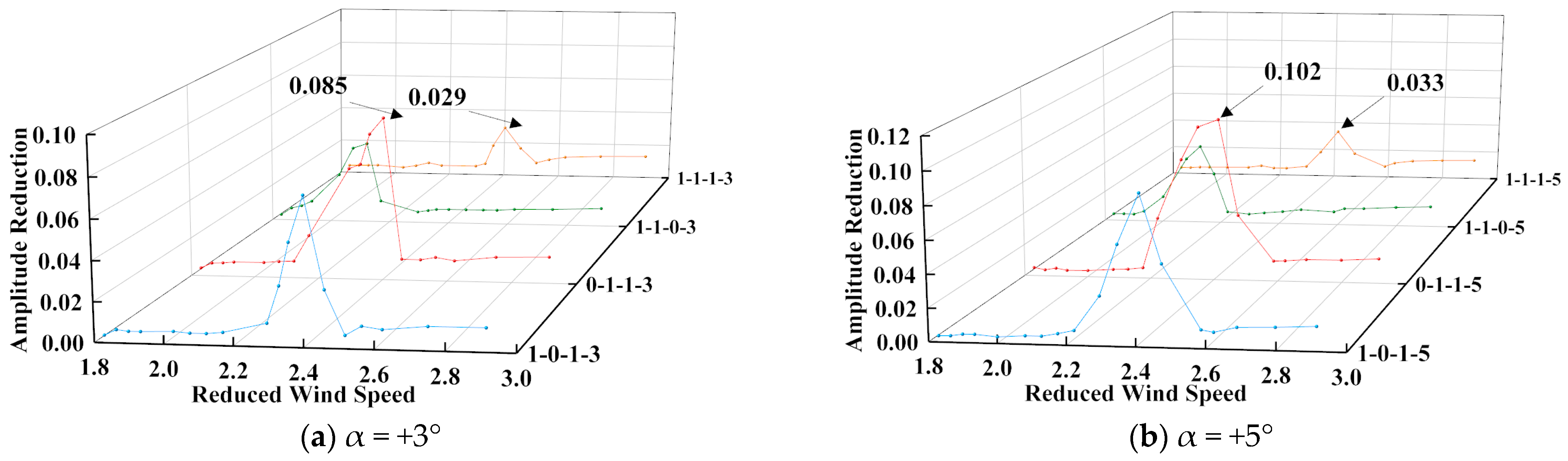
4.3.3. Vibration Suppression Rule for Combined Measures

To investigate the suppression rule of the VIV of the DDST girder through the combination of three different additional aerodynamic measures, namely, wind nozzle, deflector plate, and central stabilizer plate, four additional aerodynamic measure combinations of “upper chord nozzle + central stabilizer plate,” “belly and lower chord deflector + central stabilizer plate,” “upper chord nozzle + belly bar and lower chord deflector “ and “upper chord nozzle + belly bar and lower chord deflector + central stabilizer plate” are set up.

The optimal nozzle parameters in Section 4.3.1 are adopted for the size of the wind nozzle, and the optimal deflector parameters in Section 4.3.2 are adopted for the size of the deflector. The specific simulated working conditions of the combination of additional aerodynamic measures are shown in

Table 5. Additional aerodynamic measure combination of simulation working conditions.

Condition Number *	Wind Nozzle Angle	Wind Nozzle tip Position	Deflector Height Ratio	Stabilizer Plate Height	Wind Attack Angle
SC1-0-1-3	60°	0.50	/	45.5	+3°
SC0-1-1-3	/	/	2	45.5	+3°
SC1-1-0-3	60°	0.50	2	/	+3°
SC1-1-1-3	60°	0.50	2	45.5	+3°
SC1-0-1-5	60°	0.50	/	45.5	+5°
SC0-1-1-5	/	/	2	45.5	+5°
SC1-1-0-5	60°	0.50	2	/	+5°
SC1-1-1-5	60°	0.50	2	45.5	+5°

* The first three numbers in the working condition number, respectively, represent the presence or absence of the wind nozzle, deflector, and central stabilizer plate, where “1” indicates existence, “0” indicates none, and the fourth number represents the wind attack angle. For example, “SC1-0-1-3” represents the simulated working condition of the combination of the wind nozzle and the central stabilization plate.

. The specific VIV response of the simulated conditions for setting up the eight combination measures is shown in Figure 20.

As can be seen from Figure 20, when the combination of “belly bar and lower chord deflector + central stabilizer plate” is adopted, at +3° and +5° wind attack angles, the maximum reduction amplitudes are 0.085 and 0.102, respectively, which are reduced by 71.6% and 72.8% compared with the original section. When the combination of “upper chord nozzle + belly rod and lower chord deflector + central stabilizer plate” is used, the maximum reduction amplitude is 0.029 and 0.033, respectively, at +3° and +5° wind attack angles, which are 90.2% and 91.1% less than the original section, respectively. When the section of the DDST girder is equipped with a deflector plate and a central stabilizer plate, the upper chord wind nozzle is added, and the maximum reduction amplitude is reduced by 65.6% and 67.0%, respectively, at the +3° and +5° wind attack angles. When the upper chord nozzle and the deflector of the belly and lower chord are installed at the same time on the section of the DDST girder, the central stabilizer plate is added, and the maximum reduction amplitude is reduced by 34.6% and 35.8% at the +3° and +5° wind attack angles, respectively. It can be seen that the upper chord nozzle has the best effect on the VIV suppression of the DDST girder section, and the central stable plate has the worst effect on the VIV suppression of the DDST girder section.

We use three forms of additional aerodynamic measures: wind nozzle, deflector plate, and central stabilizer plate. The following VIV suppression mechanism is derived:

(1)

After setting up the upper chord deflector plate, the separation point of the airflow at the front edge of the upper bridge deck was advanced, resulting in stronger vortex shedding. At the same time, the “unloading effect” of the leeward side guide plate weakens the energy of the vortex in the wake area of the upper bridge deck. Under the combined action of the two, the vertical bending VIV response of the DDST girder increases slightly.

(2)

After setting up the upper chord wind nozzle, the separated flow at the front edge of the upper bridge deck adheres to the surface of the wind nozzle. More airflow escapes from the gap of the railing, resulting in a significant reduction in the vortex intensity above the upper bridge deck and significant suppression of the vertical bending VIV of the DDST girder.

(3)

The “unloading effect” of the lower chord deflector plate significantly weakens the vortex strength in the wake area of the lower bridge deck, resulting in significant suppression of the torsional vortex response of the DDST girder, especially under high wind speeds.

(4)

After setting up the central stabilizer plate, a larger flow field appeared in front of it, further consuming the energy of the airflow and causing a slight reduction in the vertical bending VIV response. In addition, the central stabilizer plate effectively reduces the frequency of vortex shedding, resulting in the vertical bending VIV locking interval length towards higher wind speeds.

5. Prediction of VIV Response of the DDST Girder Section

5.1. Amplitude Prediction of DDST Girder Section

Based on SVR, BPNN and RF, three machine learning algorithms are used to establish the prediction model and optimize the model parameters through the cross-validation method. The values of cross-validation folds are 4, 6, 8 and 10, and the minimum RMSE is used as the evaluation index for the optimization of various models; the results of the optimal values of various parameters after optimization are shown in

Table 6. Optimization results of model parameters of different machine algorithms.

Model	Parameter	Search Space	Optimal Parameter	Optimal Cross-Fold
SVR	C	{0.1~10.0}	10.0	10
	γ	{0.1~10.0}	10.0
BPNN	hidden layer	{1, 2, 3}	2	10
	hidden layer node	{5~50}	[13,6]
RF	n	{50~200}	120	10
	leaf	{1~20}	1

.

For the amplitude prediction of the DDST girder section under different wind speeds, the wind angle, reduced wind speed, upper chord wind nozzle angle, upper chord wind nozzle tip position, belly bar deflector plate height ratio, lower chord deflector plate height ratio, and central stabilizer plate height are used as feature inputs. The vertical bending reduced amplitude is used as the output. The dataset used for the amplitude prediction of the DDST girder section is defined as VIV-A. To compare the prediction effects of the three models, the VIV-A dataset was divided into training and test sets according to 9:1. The model parameters were set according to the parameters when the minimum RMSE was obtained under 10-fold cross-validation. The amplitude prediction results are shown in Figure 21, and a comparison between the predicted and actual values of amplitude is shown in Figure 22.

The data points of the SVR model are uniformly distributed on both sides of the reference line when the amplitude is small and mainly distributed on the lower side of the reference line when the amplitude is significant; the data points of the BPNN model are uniformly distributed on both sides of the reference line; and the data points of the RF model are concentrated on the reference line when the amplitude is low and deviated to the lower-right side when the amplitude is large. The amplitude prediction should be conservative; the RMSE of the BPNN prediction is 0.197, and the R² is 0.9723. Therefore, the BPNN model is the best for the amplitude prediction of the DDST girder under different wind speeds.

Since the initial weights of BPNN are random, the prediction results of each time are affected by the initial weights. Therefore, the genetic algorithm and particle swarm optimization are introduced to optimize the BPNN model to obtain higher prediction accuracy. The GA and PSO algorithms are combined with BPNN to establish the GA-BPNN and PSO-BPNN models, and the specific operation flow of the optimized model is shown in Figure 23.

Table 7. Optimization results of model parameters of different BPNN machine algorithms.

Model	RMSE	Variation Range	R2	Variation Range
BPNN	0.197	/	0.9723	/
GA-BPNN	0.150	−23.9%	0.9898	1.8%
PSO-BPNN	0.164	−16.8%	0.9878	1.6%

gives the magnitude of change in the RMSE and R² of the BPNN model before and after optimization to quantify the model’s optimization effect.

The GA-BPNN and PSO-BPNN models have improved prediction accuracy compared to the BPNN model, and the RMSEs of the GA-BPNN and PSO-BPNN models are 0.150 and 0.164, respectively, which are reduced by 23.9% and 16.8% compared to the BPNN model; the R² of the GA-BPNN and PSO-BPNN models is 0.9898 and 0.9878, indicating that the prediction performance of the optimized models has been improved, 0.9898 and 0.9878, respectively, which are 1.8% and 1.6% higher than the BPNN model, indicating that the prediction performance of the optimized models is improved. Among them, the GA-BPNN model is more suitable for predicting the amplitude of the DDST girder section under different wind speeds.

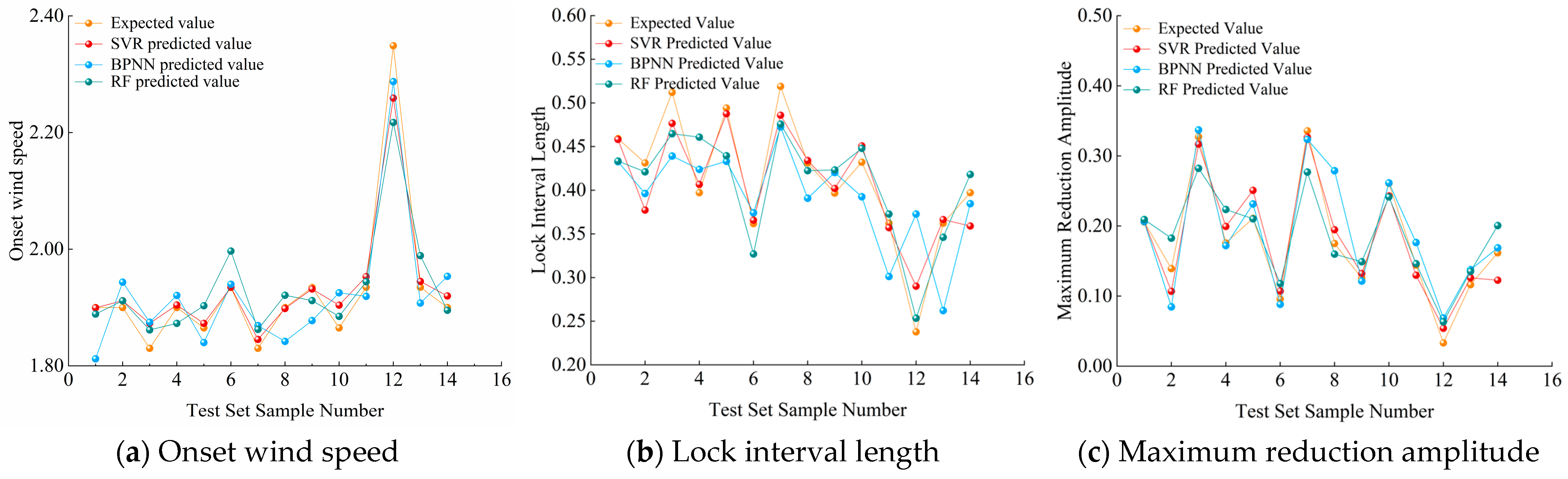
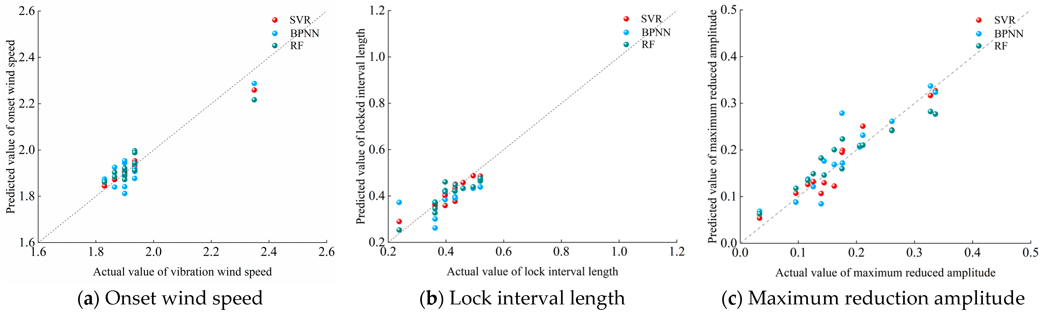
5.2. Characteristic Parameter Prediction of VIV of DDST Girder Section

For the prediction of VIV characteristic parameters of the DDST girder section under different additional aerodynamic measures, the wind attack angle, upper chord wind nozzle angle, upper chord wind nozzle tip position, belly bar deflector plate height ratio, lower chord deflector plate height ratio, and central stabilizer plate height are used as feature inputs, and the VIV onset wind speed, locking interval length, and maximum reduction amplitude are used as feature inputs. The dataset used for predicting the VIV characteristic parameters of DDST girder sections is defined as VIV-R.

To ensure the validity of the prediction results, the model built each time predicts only one feature parameter. The VIV-R dataset has 58 sets of sample data, to ensure that there are enough samples for training in each fold, so 4-fold cross-validation pairs are used for the optimization search. The specific optimization search results are shown in Figure 24, Figure 25 and Figure 26.

The VIV-R dataset was divided into training and test sets according to 3:1, and the optimal parameter settings were used to build the prediction model. The prediction results of the VIV characteristic parameters are shown in Figure 27, and a comparison between the predicted and actual values of the VIV characteristic parameters is shown in Figure 28.

The RMSE predicted by the SVR model for the VIV onset wind speed, locking interval length, and maximum reduction amplitude of the DDST girder section was the smallest, at 0.026, 0.024, and 0.393, respectively.

The predictions of the VIV characteristic parameters of the SVR model are all concentrated on the reference line, and most of the predictions of the VIV characteristic parameters of the BPNN and RF models are close to the reference line. The SVR model has higher credibility for the prediction of VIV characteristic parameters, and the BPNN and RF models have some credibility. The R² of the prediction of VIV characteristic parameters of the SVR model is the largest, at 0.9398, 0.8520, and 0.9299, respectively. Therefore, in the case of a small sample size of the additional aerodynamic measures condition, the SVR model has the best prediction of the onset wind speed of the VIV of the DDST girder section, locking interval length, and maximum reduction amplitude.

The SVR model is optimized by combining GA and PSO, and the RMSE and R² values of the model before and after optimization are shown in

Table 8. Optimization results of model parameters of different SVR machine algorithms.

Model	Parameter	RMSE	Variation Range	R2	Variation Range
SVR	Onset wind speed	0.026	/	0.9398	/
	Lock interval length	0.024	/	0.8520	/
	Maximum reduction Amplitude	0.393	/	0.9299	/
GA-SVR	Onset wind speed	0.019	−26.9%	0.9290	−1.1%
	Lock interval length	0.022	−8.3%	0.8748	2.7%
	Maximum reduction Amplitude	0.315	−19.8%	0.9475	1.9%
PSO-SVR	Onset wind speed	0.017	−34.6%	0.9421	0.2%
	Lock interval length	0.026	−19.8%	0.8875	4.2%
	Maximum reduction Amplitude	0.295	−24.9%	0.9462	1.8%

.

Overall, the optimized model has higher accuracy and stability than the original model. Among them, the PSO-SVR model is more suitable for predicting the characteristic parameters of the VIV of the DDST girder section. The RMSEs for the prediction of onset wind speed, locking interval length, and maximum reduction amplitude are 0.017, 0.026 and 0.295, respectively, which are 34.6%, -19.8% and 24.9% less than that of the SVR model; the R² is 0.9421, 0.8875 and 0.9462, at 0.2%, 4.2% and 1.8% more than that of the original model due to the small sample size and the bias of the data. A smaller sample size leads to data bias appearing; RMSE increases, and R² decreases.

Calculating a single working condition using numerical simulation methods takes about 6 h, while the improved algorithm models GA-BPNN and PSO-SVR take into account both accuracy and efficiency. For a sample, the prediction time is only about 3 s.

6. Conclusions

(1)

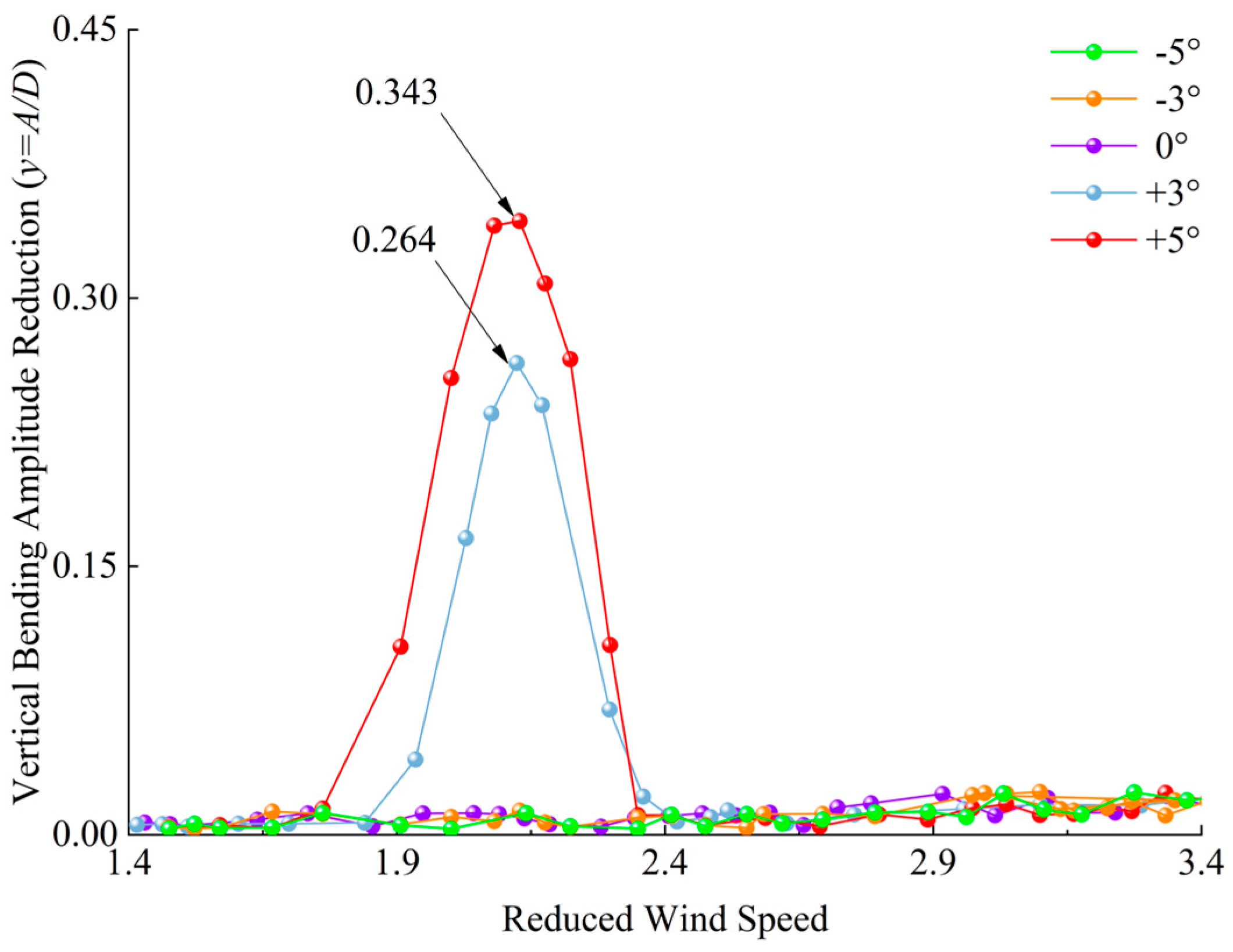
In the VIV test, the segmental model will have vertical bending VIV at +3° and +5° wind angles of attack. The increase in the wind angle of attack leads to an increase in the locking interval length and maximum reduction amplitude, and the reduction wind speed of vibration onset is advanced.

(2)

Numerical simulation of the DDST girder was carried out to investigate the vertical bending VIV response of the section after changing the parameters of different additional aerodynamic measures and to summarize the effects of these variables on the VIV performance, which can provide reliable samples for the machine algorithm model.

(3)

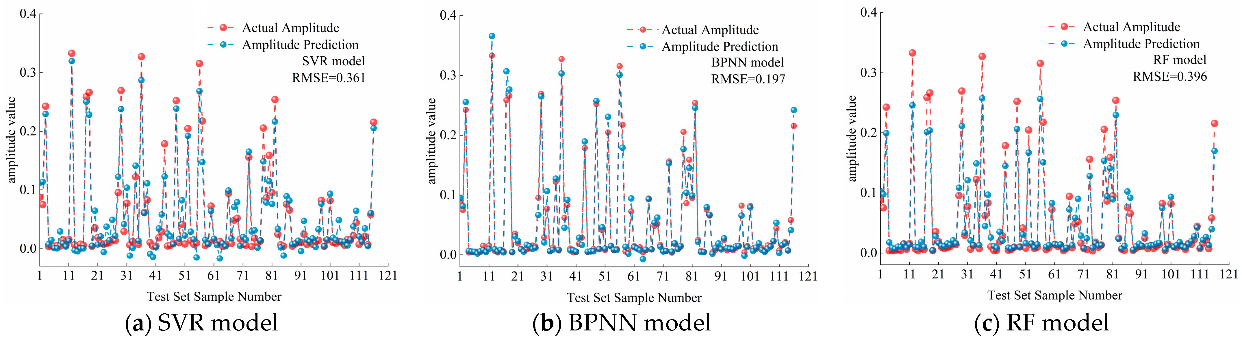
The VIV data obtained from the numerical simulation are organized to establish the VIV-A and VIV-R datasets, and the prediction models are established by combining the three algorithms. Among them, the BPNN model predicts the amplitude best, and the SVR model predicts the VIV characteristic parameters with the best agreement.

(4)

The BPNN and SVR algorithms are improved and optimized by combining the GA and PSO algorithms, respectively, and the results show that the GA-BPNN model predicts the amplitude better than the BPNN model, and the PSO-SVR model predicts the VIV characteristic parameters better than the SVR model, which proves the validity of the improved algorithms. Compared with the wind tunnel test and numerical simulation, the proposed prediction model can significantly improve the computational efficiency while considering the computational accuracy.

References

- Wang, B.; Li, W.; Zhao, C.; Zhang, Q.; Li, G.; Liu, X.; Yan, B.; Cai, X.; Zhang, J.; Zheng, S. L2-Norm Quasi 3-D Phase Unwrapping Assisted Multitemporal InSAR Deformation Dynamic Monitoring for the Cross-Sea Bridge. IEEE J. Sel. Top. Appl. Earth Obs. Remote Sens. 2024, 17, 18926–18938. [Google Scholar] [CrossRef]
- Hong, C.; Lyu, Z.; Wang, F.; Zhao, Z.; Wang, L. Wave-Current Loads on a Super-Large-Diameter Pile in Deep Water: An Experimental Study. Appl. Sci. 2023, 13, 8859. [Google Scholar] [CrossRef]
- Gao, D.; Deng, Z.; Yang, W.; Chen, W. Review of the Excitation Mechanism and Aerodynamic Flow Control of Vortex-Induced Vibration of the Main Girder for Long-Span Bridges: A Vortex-Dynamics Approach. J. Fluids Struct. 2021, 105, 103348. [Google Scholar] [CrossRef]
- Hu, C.; Zhao, L.; Wang, X.; Ge, Y. Spatio-Temporal Distribution of Aerodynamic Forces and Their Associated Vortex Drift Patterns around a Closed-Box Girder during Torsional Vortex-Induced Vibration. Eng. Struct. 2024, 302, 117459. [Google Scholar] [CrossRef]
- Zhong, Y.; Li, M.; Ma, C. Aerodynamic Admittance of Truss Girder in Homogenous Turbulence. J. Wind Eng. Ind. Aerodyn. 2018, 172, 152–163. [Google Scholar] [CrossRef]
- Xin, D.; Zhan, J.; Zhang, H.; Ou, J. Control of Vortex-Induced Vibration of a Long-Span Bridge by Inclined Railings. J. Bridge Eng. 2021, 26, 04021093. [Google Scholar] [CrossRef]
- Zhang, T.; Sun, Y.; Li, M.; Yang, X. Experimental and Numerical Studies on the Vortex-Induced Vibration of Two-Box Edge Girder for Cable-Stayed Bridges. J. Wind Eng. Ind. Aerodyn. 2020, 206, 104336. [Google Scholar] [CrossRef]
- Wu, Y.; Wu, X.; Li, J.; Xin, H.; Sun, Q.; Wang, J. Investigation of Vortex-Induced Vibration of a Cable-Stayed Bridge without Backstays Based on Wind Tunnel Tests. Eng. Struct. 2022, 250, 113436. [Google Scholar] [CrossRef]
- Wang, W.; Cao, S. Numerical Study of Aerodynamic Roles of Bridge Railings by Immersed Boundary Method. J. Wind Eng. Ind. Aerodyn. 2022, 228, 105111. [Google Scholar] [CrossRef]
- Duan, Q.; Ma, C.; Li, Q. Vortex-Induced Vibration Performance and Mechanism of Long-Span Railway Bridge Streamlined Box Girder. Adv. Struct. Eng. 2023, 26, 2506–2519. [Google Scholar] [CrossRef]
- Fang, C.; Hu, R.; Tang, H.; Li, Y.; Wang, Z. Experimental and Numerical Study on Vortex-Induced Vibration of a Truss Girder with Two Decks. Adv. Struct. Eng. 2020, 24, 136943322096902. [Google Scholar] [CrossRef]
- Tang, H.; Shum, K.M.; Tao, Q.; Jiang, J. Vortex-Induced Vibration of a Truss Girder with High Vertical Stabilizers. Adv. Struct. Eng. 2019, 22, 948–959. [Google Scholar] [CrossRef]
- Li, M.; Lin, Z.; Dai, R.; Wang, Y.; Li, M. Effects of Wind Barriers on the Aerodynamic Forces and Driving Safety of Vehicles on a Wide Bridge Girder at Various Angles of Attack. Phys. Fluids 2024, 36, 105109. [Google Scholar] [CrossRef]
- Bai, H.; Ji, N.; Xu, G.; Li, J. An Alternative Aerodynamic Mitigation Measure for Improving Bridge Flutter and Vortex Induced Vibration (VIV) Stability: Sealed Traffic Barrier. J. Wind Eng. Ind. Aerodyn. 2020, 206, 104302. [Google Scholar] [CrossRef]
- Xu, F.; Ying, X.; Li, Y.; Zhang, M. Experimental Explorations of the Torsional Vortex-Induced Vibrations of a Bridge Deck. J. Bridge Eng. 2016, 21, 04016093. [Google Scholar] [CrossRef]
- Zhan, J.; Xin, D.; Ou, J.; Liu, Z. Experimental Study on Suppressing Vortex-Induced Vibration of a Long-Span Bridge by Installing the Wavy Railings. J. Wind Eng. Ind. Aerodyn. 2020, 202, 104205. [Google Scholar] [CrossRef]
- Yang, Y.; Li, L.; Yao, G.; Wang, M.; Zhou, C.; Lei, T.; Tan, H. Study on the Influence of the Fully Enclosed Barrier on the Vortex-Induced Vibration Performance of a Long-Span Highway-Railway Double-Deck Truss Bridge. Phys. Fluids 2024, 36, 087132. [Google Scholar] [CrossRef]
- Pawar, S.; Rahman, S.M.; Vaddireddy, H.; San, O.; Rasheed, A.; Vedula, P. A Deep Learning Enabler for Nonintrusive Reduced Order Modeling of Fluid Flows. Phys. Fluids 2019, 31, 085101. [Google Scholar] [CrossRef]
- Lusch, B.; Kutz, J.N.; Brunton, S.L. Deep Learning for Universal Linear Embeddings of Nonlinear Dynamics. Nat. Commun. 2018, 9, 4950. [Google Scholar] [CrossRef]
- Wei, S.; Jin, X.; Li, H. General Solutions for Nonlinear Differential Equations: A Rule-Based Self-Learning Approach Using Deep Reinforcement Learning. Comput. Mech. 2019, 64, 1361–1374. [Google Scholar] [CrossRef]
- Yan, Z.; Zheng, S.; Tai, X.; Yang, F.; Ding, Z. Machine Learning Models for Predicting VIV Amplitude of Streamlined Steel Box Girders. Structures 2024, 63, 106444. [Google Scholar] [CrossRef]
- Li, S.; Laima, S.; Li, H. Physics-Guided Deep Learning Framework for Predictive Modeling of Bridge Vortex-Induced Vibrations from Field Monitoring. Phys. Fluids 2021, 33, 037113. [Google Scholar] [CrossRef]
- Yan, W.-J.; Feng, Z.-Q.; Yang, W.; Yuen, K.-V. Bayesian Inference for the Dynamic Properties of Long-Span Bridges under Vortex-Induced Vibration with Scanlan’s Model and Dense Optical Flow Scheme. Mech. Syst. Signal Process. 2022, 174, 109078. [Google Scholar] [CrossRef]
- Fluent User’s Guide. Available online: https://ansyshelp.ansys.com/Views/Secured/corp/v221/en/flu_ug/flu_ug.html (accessed on 27 March 2025).
- Siedziako, B.; Øiseth, O. On the Importance of Cross-Sectional Details in the Wind Tunnel Testing of Bridge Deck Section Models. Procedia Eng. 2017, 199, 3145–3151. [Google Scholar] [CrossRef]
- Li, S.; Laima, S.; Li, H. Data-Driven Modeling of Vortex-Induced Vibration of a Long-Span Suspension Bridge Using Decision Tree Learning and Support Vector Regression. J. Wind Eng. Ind. Aerodyn. 2018, 172, 196–211. [Google Scholar] [CrossRef]
- Lu, Y.; Luo, Q.; Liao, Y.; Xu, W. Vortex-Induced Vibration Fatigue Damage Prediction Method for Flexible Cylinders Based on RBF Neural Network. Ocean Eng. 2022, 254, 111344. [Google Scholar] [CrossRef]
- Xu, W.; He, Z.; Zhai, L.; Wang, E. Vortex-Induced Vibration Prediction of an Inclined Flexible Cylinder Based on Machine Learning Methods. Ocean Eng. 2023, 282, 114956. [Google Scholar] [CrossRef]
- Hu, G.; Kwok, K.C.S. Predicting Wind Pressures around Circular Cylinders Using Machine Learning Techniques. J. Wind Eng. Ind. Aerodyn. 2020, 198, 104099. [Google Scholar] [CrossRef]
- Sun, H.; Zhu, L.-D.; Tan, Z.-X.; Zhu, Q.; Meng, X.-L. Spanwise Layout Optimization of Aerodynamic Countermeasures for Multi-Mode Vortex-Induced Vibration Control on Long-Span Bridges. J. Wind Eng. Ind. Aerodyn. 2024, 244, 105616. [Google Scholar] [CrossRef]
- Chen, Z.; Zhang, L.; Li, K.; Xue, X.; Zhang, X.; Kim, B.; Li, C.Y. Machine-Learning Prediction of Aerodynamic Damping for Buildings and Structures Undergoing Flow-Induced Vibrations. J. Build. Eng. 2023, 63, 105374. [Google Scholar] [CrossRef]
- Wang, Z.; Zhu, J.; Zhang, Z. Machine Learning-Based Deep Data Mining and Prediction of Vortex-Induced Vibration of Circular Cylinders. Ocean Eng. 2023, 285, 115313. [Google Scholar] [CrossRef]
- Zhao, D.; Shao, Y.; Hu, H.; Hu, G.; Wang, Y. RBF-PSO-IS: An Innovative Metamodeling for Reliability Analysis of Bridge’s Vortex-Induced Vibration. Structures 2023, 55, 59–70. [Google Scholar] [CrossRef]
- Matlab. Available online: https://ww2.mathworks.cn/help/matlab/index.html?s_tid=hc_panel (accessed on 27 March 2025).
- Zhang, Y.-M.; Wang, H.; Bai, Y.; Mao, J.-X.; Chang, X.-Y.; Wang, L.-B. Switching Bayesian Dynamic Linear Model for Condition Assessment of Bridge Expansion Joints Using Structural Health Monitoring Data. Mech. Syst. Signal Process. 2021, 160, 107879. [Google Scholar] [CrossRef]