Article

Gross Tonnage-Based Statistical Modeling and Calculation of Shipping Emissions for the Bosphorus Strait

by
Kaan Ünlügençoğlu
Department of Marine Engineering Operations, Naval Architecture and Maritime Faculty, Yıldız Technical University, Istanbul 34349, Türkiye
J. Mar. Sci. Eng. 2025, 13(4), 744; https://doi.org/10.3390/jmse13040744
Submission received: 11 March 2025 / Revised: 26 March 2025 / Accepted: 3 April 2025 / Published: 8 April 2025
(This article belongs to the Section Marine Environmental Science)

Abstract

:
Maritime transportation is responsible for most global trade and is generally considered more environmentally efficient compared to other modes of transport, particularly for long-distance trade. With increasingly stringent emission regulations, however, accurately quantifying emissions and identifying their key determinants has become essential for effective environmental management. This study introduced a structured and comparative statistical modeling framework for ship-based emission modeling using gross tonnage (GT) as the primary predictor variable, due to its strong correlation with emission levels. Emissions for hydrocarbon (HC), carbon monoxide (CO), particulate matter with an aerodynamic diameter of less than 10 μm (PM10), carbon dioxide (CO2), sulfur dioxide (SO2), nitrogen oxides (NOx), and volatile organic compounds (VOC) were estimated using a bottom-up approach based on emission factors and formulas defined by the U.S. Environmental Protection Agency (EPA), using data from 38,304 vessel movements through the Bosphorus in 2021. These EPA-estimated values served as dependent variables in the modeling process. The modeling framework followed a three-step strategy: (1) outlier detection using Rosner’s test to reduce the influence of outliers on model accuracy, (2) curve fitting with 12 regression models representing four curve types—polynomial (e.g., linear, quadratic), concave/convex (e.g., exponential, logarithmic), sigmoidal (e.g., logistic, Gompertz, Weibull), and spline-based (e.g., cubic spline, natural spline)—to capture diverse functional relationships between GT and emissions, and (3) model comparison using difference performance metrics to ensure a comprehensive assessment of predictive accuracy, consistency, and bias. The findings revealed that nonlinear models outperformed polynomial models, with spline-based models—particularly natural spline and cubic spline—providing superior accuracy for HC, PM10, SO2, and VOC, and the Weibull model showing strong predictive performance for CO and NOx. These results underscore the necessity of using pollutant-specific and flexible modeling strategies to capture the intricacies of maritime emission dynamics. By demonstrating the advantages of flexible functional forms over standard regression techniques, this study highlights the need for tailored modeling strategies to better capture the complex relationships in maritime emission data and offers a scalable and transferable framework that can be extended to other vessel types, emission datasets, or maritime regions.

1. Introduction

With the expansion of global trade, maritime transportation has become the dominant mode of transport due to its reliability, efficiency, and cost-effectiveness, accounting for approximately 90% of global trade volume [1,2]. However, the environmental impacts of frequent shipping activities, particularly on air and water quality, have raised significant concerns among various stakeholders. Shipping activities contribute to approximately 15% of global NOx emissions, 13% of SOx emissions, and 3% of CO2 emissions annually [3]. In light of these concerns, the International Maritime Organization (IMO) has prioritized strategies to mitigate air pollution by emphasizing the reduction in ship-based emissions. Regulating ship emissions under international standards requires the measurement, reporting, and verification of emission values. Strict monitoring by regulatory bodies has prompted substantial changes in the maritime industry. Ship emissions, particularly in coastal areas, are known to adversely affect public health, with approximately 70% of global ship emissions occurring within 400 km of coastal zones [4]. In addition to their environmental and public health impacts, ship emissions also incur significant economic costs, with studies highlighting their contribution to health expenditures and environmental damage [5]. To support international climate goals such as those outlined in the Paris Agreement, the IMO has introduced both short- and long-term regulatory strategies, including the Energy Efficiency Existing Ship Index (EEXI) and the Carbon Intensity Indicator (CII) [6,7]. Effective implementation of these strategies is expected to reduce environmental pollution, improve public health through enhanced air quality, and promote sustainable maritime operations, contributing to long-term global economic and environmental stability.
The Bosphorus, located in the Marmara Region of Türkiye, is one of the country’s busiest and most strategically important maritime routes. Beyond its geographical significance, the strait holds substantial ecological value due to its unique marine and terrestrial ecosystems [8]. Residents of Istanbul’s densely populated coastal districts are particularly vulnerable to ship-based emissions, highlighting the urgent need for effective mitigation strategies in the area. In 2021 alone, 38,304 ships transited the Bosphorus, making it one of the most heavily trafficked maritime corridors in the region. This intense shipping activity has led to significant environmental challenges, particularly in terms of air pollution. Given the high costs and time demands associated with direct emission measurements, empirical formulas—such as those developed by the U.S. EPA and used to calculate emission values prior to statistical modeling in this study—offer an efficient and scalable alternative for estimating emissions.
The detrimental effects of shipping emissions concern not only air quality [9,10,11] but also public health [12,13]. This growing concern has driven scientific efforts to develop strategies to mitigate these impacts [14,15]. In response to the growing interest in accurately estimating emissions, numerous studies have employed bottom-up, top-down, and hybrid methodologies to evaluate ship emissions. Bottom-up approaches are commonly used to develop detailed activity-based emissions inventories, while top-down methods estimate emissions based on aggregated fuel consumption data. Each method offers unique strengths and weaknesses, with the bottom-up approach delivering highly detailed and precise results by incorporating specific ship activities; however, it demands substantial and accurate data, which makes it both time-intensive and resource-heavy. In contrast, the top-down approach requires less detailed data and is more appropriate for large-scale as well as global studies; however, its dependence on aggregated fuel consumption data can result in reduced accuracy, especially when applied at local or operational scales. To enhance accuracy and address methodological challenges, several studies have also combined these approaches as hybrid modeling.
Numerous studies have been conducted using bottom-up, top-down, and hybrid methodologies and provided valuable insights into emission estimation accuracy and applicability across different contexts. For example, Ekmekçioğlu et al. [16] constructed a detailed activity-based emissions inventory for the Ambarlı and Kocaeli ports using the Euro North Atlantic Treaty Organization (NATO) Training Engineer Centre (ENTEC) calculation method across multiple operational modes. Similarly, Yang et al. [17] and Toscano et al. [18] employed bottom-up methods using the Automatic Identification System (AIS) data for ports in China and Italy, respectively, with both focusing on pollutant characteristics and local air quality impacts. Meanwhile, Kuzu et al. [19] combined emissions estimation with dispersion modeling and environmental cost analysis at Bandırma Port in Türkiye using fuel consumption data. These studies highlighted the importance of both bottom-up and top-down methodologies but also revealed challenges related to data availability and accuracy, particularly for local-scale emissions inventories. Kanberoğlu and Kökkülünk [20] proposed a novel energy efficiency indicator for assessing fleet energy performance. Their study utilized real-world data collected from five bulk carrier ships between 2017 and 2018, with CO2 emissions calculated using a top-down approach. Similarly, Kılıç et al. [21] focused on various ship types, including bulk carriers, general cargo vessels, container ships, roll-on/roll-off (ro-ro) cargo ships, and chemical/oil tankers anchored at Iskenderun Port. Using a top-down approach, they estimated NOx, particulate matter (PM), CO, volatile organic compound (VOC), CO2, and SO2 emissions and highlighted the significant environmental and economic advantages of utilizing shore-side electricity over auxiliary engines. Several notable studies have also contributed to the literature by employing both bottom-up and top-down methods simultaneously to calculate emissions. For example, Endresen et al. [22] developed emissions inventories for CO2 and SO2 pollutants spanning from 1925 to 2002 using an activity-based approach, while inventories for the same pollutants were constructed from 1970 to 2000 using a fuel-based approach. Bilgili and Celebi [23] utilized real-time noon reports from nine bulk carriers and various methodologies based on fuel consumption, engine power, and energy use to calculate NOx, CO, SOx, particles less than 2.5 µm in diameter (PM2.5), CO2, CH4, and N2O emissions. Similarly, Ekmekçioğlu et al. [11] used a fuel-based approach across four operational modes (i.e., port, maneuvering, cruising, anchorage) to estimate NOx, non-methane VOC (NMVOC), PM, SOx, CO, and CO2 emissions. Their study also compared the estimations of the utilized approaches, providing valuable insights into the accuracy levels of the two models.
In addition to studies focusing on the quantification of emissions and the effects of pollutants from maritime activities, statistical modeling research has also significantly contributed to identifying the key predictors of calculated emissions. These studies have employed various methodologies, including traditional statistical techniques such as linear regression [23,24,25] and nonlinear regression [26,27] models. More recently, machine learning methods [28] have been introduced as alternatives to traditional regression techniques, as they offer such advantages as reduced assumptions and improved flexibility in specific contexts. However, nonlinear regression models are still widely used in environmental modeling due to their ability to capture diverse data patterns (e.g., saturation effects, growth curves, multiple inflection points) while providing parameters that are often directly interpretable in the context of the process being studied. By considering these patterns, various nonlinear curve types have been developed to better represent complex relationships in environmental datasets, including those with non-monotonic and threshold behaviors. Despite the predominant use of polynomial regression in the literature, polynomial models can oversimplify relationships by assuming continuous and smooth patterns, which may not align with real-world emissions behaviors. Therefore, exploring diverse nonlinear models (e.g., polynomial curves, concave/convex, sigmoidal, flexible spline shapes) remains essential for uncovering intricate patterns and improving the accuracy of predictive models, particularly with regard to complex environmental datasets.
Identifying the appropriate curve type for modeling emission patterns first requires accurately determining the key predictors of emissions, as the choice of regression models depends on the nature and strength of these relationships. Trozzi [29] highlighted a positive correlation between a ship’s gross tonnage (GT) and machinery power, emphasizing that emissions tend to increase with higher tonnage due to greater engine power and load-carrying capacity. Given that ships exceeding 500 GT produce over half of the air pollution emissions (particularly NOx, SOx, and CO2) [30], GT-based approaches offer a valuable framework for estimating emissions during the ship design process. Building upon these studies, this research aims to provide a broader perspective on GT-based modeling approaches and contributes to the existing literature by evaluating how well different statistical models represent the EPA-estimated emissions based on ship characteristics. In doing so, the present study addresses a notable gap in the literature by implementing and systematically comparing an extensive range of nonlinear regression forms, several of which—such as spline-based models [31] have not previously been applied in maritime emission modeling.
This study uses a bottom-up approach to calculate the HC, CO, PM10, CO2, SO2, NOx, and VOC emissions from various types of ships transiting the Bosphorus in 2021. These emissions are calculated for each of the 38,304 vessel transits based on ship-specific parameters obtained from real-time AIS-based monitoring and the U.S. EPA methodology. To investigate the relationship between GT and emissions in greater detail, the study implements a structured and comparative three-step statistical modeling framework specifically for general cargo vessels, which represent the most frequently observed ship type in the dataset. This framework uses EPA-estimated emission values as inputs to identify the most appropriate functional forms for maritime emission modeling. The first step is to identify and remove outliers to mitigate potential biases when estimating the parameters of the regression models. The second step employs 12 regression models, representing a variety of curve types, to investigate both the linear and nonlinear relationships each emission factor has with GT. These include polynomial models (linear regression, quadratic regression, cubic regression), concave/convex models (exponential regression, logarithmic regression), sigmoidal models (three-parameter logistic regression, four-parameter logistic regression, Gompertz regression, Weibull regression), and flexible spline models (cubic spline, natural spline). The rationale for using such a wide range of curve types stems from the need to capture the complex, nonlinear dynamics that characterize the relationship between ship size and emissions. The third and final step involves evaluating and comparing the performances of the estimated regression models to identify the most accurate and robust representations of the observed emission patterns, with the aim being to contribute to more precise and reliable emissions estimation frameworks for maritime applications. To the authors’ knowledge, this is one of the first studies to systematically assess and compare such a broad array of nonlinear curve types using actual emissions data derived from a high-traffic waterway. Notably, spline-based regression models remain largely underexplored in maritime emission modeling, further underscoring the methodological novelty of this research. Furthermore, the framework establishes a transparent and replicable structure that supports comparative modeling efforts across different vessel categories, regions, or explanatory variables, thus contributing a scalable methodological template to the maritime emissions literature.
Section 2 goes on to provide a comprehensive description of the dataset used in the study and includes a detailed breakdown of vessel transits categorized by ship type and traffic direction. This section elaborates on the bottom-up approach employed for emissions estimation and presents the three-step statistical modeling framework in detail. In order to ensure a comprehensive assessment of the models’ effectiveness, this section also covers the procedures for outlier analysis, the nonlinear regression models applied in the study, and the performance metrics used for model comparisons, including the criteria for evaluating goodness-of-fit and predictive accuracy. Section 3 presents the results obtained from the methodologies described in Section 2 and includes the findings from the emissions estimations and model comparisons. Lastly, Section 4 summarizes the key findings, discusses the study’s contributions to the emissions modeling literature, and offers recommendations for future research and practical applications in the maritime industry.

2. Materials and Methods

This study uses the EPA method within a bottom-up modeling framework to calculate the HC, CO, PM10, CO2, SO2, NOx, and VOC emissions from the main and auxiliary engines of ships transiting the Bosphorus. This approach incorporates a range of parameters derived from real-world data on 38,304 ship movements as provided by the Directorate General of Coastal Safety in Türkiye. A structured and comparative three-step statistical modeling framework is applied following the emissions calculations. The first step identifies the outliers in each emission dataset and removes them using Rosner’s Test, a robust method capable of detecting multiple outliers simultaneously. This ensures a refined dataset, thus reducing potential biases when estimating the regression model parameters. The second step splits the cleaned datasets into training (80%) and testing (20%) subsets and applies 12 regression models—encompassing both linear and nonlinear approaches—to the EPA-estimated emission values for each pollutant. To ensure the robustness and reliability of the models, the study implements a 10-fold cross-validation. This procedure alternates between using nine subsets for training and one for validation, iteratively covering all subsets, thereby mitigating overfitting and ensuring the generalization ability of the models to unseen data. The final step systematically evaluates and compares the performances of these models using multiple metrics involving normalized root mean square error (NRMSE), percentage bias (PBIAS), and difference in the mean absolute percentage error (MAPEdiff) to identify the most suitable model for each emission type. All statistical analyses and graphical visualizations are performed using the statistical software R (ver. 4.1.2) [32]. The following subsections provide detailed explanations of each step and their methodologies for clarity and transparency.

2.1. Dataset and Characteristics of the Bosphorus

Serving as a natural divide between the continents of Asia and Europe, the Bosphorus is a key international waterway in the Marmara Sea and one of the busiest and narrowest in the world. Beyond its strategic importance for global maritime trade, this strait significantly affects the air quality of Istanbul, a metropolitan area with approximately 16 million inhabitants who are exposed to the air pollution caused by ship-generated emissions.
To ensure safe and efficient navigation in this critical passage, a traffic separation scheme has been established in accordance with the International Regulations for Preventing Collisions at Sea (COLREG). This system organizes maritime traffic into two designated routes facilitating south-to-north (S-N) and north-to-south (N-S) movements [33]. In 2021, the strait witnessed a total of 38,304 vessel transits encompassing various types and sizes of ships, such as bulk carriers, container ships, general cargo vessels, passenger ships, roll-on/roll-off (ro-ro) ships, and tankers. Table 1 provides a detailed breakdown of these transits categorized by ship type and traffic direction.
Figure 1 highlights general cargo ships as constituting the most frequent type of passage through the Bosphorus, accounting for 43% of all transit. This is followed by bulk carriers at 24.11%, tankers at 21.58%, container ships at 7.23%, other types at 2.62%, ro-ro vessels at 1.36%, and passenger ships at 0.11%. Among these, general cargo ships dominate both the S-N and N-S directions with a nearly equal distribution of transits, making them the most significant contributor to maritime traffic in the region. The non-bold percentages displayed at the sides of the bars represent the individual share of each ship type in the S-N (blue) and N-S (red) directions separately, further confirming the balanced bidirectional movement of the most prominent ship categories.
HC, CO, PM10, CO2, SO2, NOx, and VOC emissions from the main and auxiliary engines of ships transiting the Bosphorus are calculated using the U.S. EPA method [34], which requires key parameters such as ships’ main and auxiliary engine power, GT, and transit time through the strait. These parameters have been derived from data collected during 38,304 ship transits as provided by Türkiye’s Directorate General of Coastal Safety.
This study employs a bottom-up approach—using the U.S. EPA method—to calculate ship emissions based on multiple influencing factors such as main and auxiliary engine power, engine revolution speed, fuel type, load factor, and transit time. These parameters are combined with the EPA method to calculate emission values, as represented in Equation (1) [34]:
E g = T h × M E k W × L F M E % × E F g k W h + A E k W × L F A E % × E F g k W h
where E represents the per-vessel emissions (g), T denotes the engine operating time (h), and ME and AE, respectively, refer to the main and auxiliary engine power (kW). LFME and LFAE, respectively, indicate the load factors of the main and auxiliary engines (%). EF represents the emission factor (g/kWh) for each ship type based on fuel and engine type.
While information on the main engine power, auxiliary engine power, and strait passage time for each ship have been collected as part of a comprehensive real dataset, the main engine loads are determined by dividing the strait passage speed of each vessel by its service speed. A load factor of 50% is assumed for auxiliary engines, with the operation of two generators considered during the strait passage. Calculating EF values for HC, CO, PM10, CO2, SO2, NOx, and VOC emissions are based on the EPA methodology, with Table 2 presenting the HC and CO emissions as derived from the EPA. Additionally, VOC emissions are calculated as 1.053 times a ship’s HC emissions.
EF(PM10) represents PM10 emissions adjusted for fuel sulfur (g/kWh) and is calculated using Equation (2), where PMbase denotes the base EF, which is fixed at 0.1545 g/kWh for marine diesel oil (MDO) and 0.5761 g/kWh for heavy fuel oil (HFO). Actual fuel sulfur levels are indicated by Sact, which is set at 0.005 for all vessel activity outside the emission control area (ECA) as of 2020. Brake specific fuel consumption (BSFC) rates are selected based on Table 3. The fraction of sulfur in fuel converted directly to sulfate (SO2) PM is represented as FSC and equals 0.02247. The molecular weight ratio of SO2 PM to sulfur is denoted as MWR and equals 7.
E F P M 10 = P M b a s e + S a c t × B S F C × F S C × M W R
EF(CO2) represents the emission factor for CO2 (g/kWh) and is calculated using Equation (3). The BSFC rates provided in Table 3 are used in the calculation. The carbon content factor (CCF) is fixed at 3.206 g CO2 per gram for MDO and 3.114 g CO2 per gram for HFO.
E F C O 2 = B S F C × C C F
EF(SO2) represents SO2 emissions (g/kWh) and is calculated using Equation (4). The BSFC rates provided in Table 3 are applied to the calculations. The fraction of sulfur in fuel converted directly to SO2 is represented as FSC and fixed at 0.97753, while the MWR of SO2 to sulfur is set at 2.
EF S O 2 = S act × B S F C × F S C × M W R
EF(NOx) varies based on ships’ year of construction, type of fuel used, and engine type, as detailed in Table 4.

2.2. Emission Estimation Methodology for Ships Transiting the Bosphorus

This study employs a structured and comparative three-step statistical framework to analyze and model ship emissions. This framework involves outlier detection to ensure data quality, regression modeling to evaluate the relationship between GT and emissions through a variety of linear and nonlinear models, and model comparisons to assess the performance and suitability of these models for each emission type. The detailed methodology for each step is described in the following subsections.

2.2.1. Outlier Detection

Just as in linear regression models, nonlinear regression models assume the distribution of least-square residuals (the vertical distance between observed and model-predicted values) to follow a Gaussian distribution. An outlier is an anomalous observation that deviates significantly from the pattern of other data points in the dataset and can introduce bias into the estimation of model parameters. Notably, most traditional statistical methods are highly sensitive to outliers, making their identification prior to the modeling process crucial.
A variety of statistical techniques are available to detect outliers in univariate data, including Dixon’s Q test, Grubb’s test, and Rosner’s test (a generalized extreme Studentized deviate [ESD] many-outlier procedure). Unlike Dixon’s Q and Grubb’s tests, Rosner’s test [35] identifies multiple outliers simultaneously and is robust against the masking effect. This study uses Rosner’s test to identify outliers in each emission data series and excludes the observations classified as outliers from further analysis.

2.2.2. Fitting Linear and Nonlinear Regression Models

Regression analysis is a fundamental statistical method used to model and explain the relationship between a dependent variable (y) and one or more predictor variables (x). Fundamentally, a regression model can be generalized as follows:
y = f x , γ + ε
where ε represents an independent and identically distributed error term, and γ denotes the unknown parameter vector of the response function f(.), characterizing the relationship between x and y. Establishing a functional relationship between x and y often involves addressing nonlinear dependencies within the model parameters. Consequently, the response function f(.) cannot be assumed to be linear in its parameters as occurs with linear regression models. Given the vast array of potential functional forms available to characterize f(.), nonlinear regression models have become essential for capturing diverse curve shapes and fitting them to real-world data. Nonlinear regression models are particularly valuable due to their ability to accommodate complex relationships between variables and provide parameters directly interpretable in the context of the studied process [36]. This interpretability in combination with their flexibility has led to their increased application across different scientific areas involving real-world data. However, identifying a suitable functional form that optimally fits the observed data remains a key challenge. To address this challenge, functions from specific curve families have been considered, such as polynomial curves, concave/convex curves, and s-shaped (sigmoidal) curves [37,38]. Additionally, flexible curves such as splines offer a data-driven approach capable of capturing complex nonlinear patterns without relying on pre-defined functional forms. These curve shapes offer a broad spectrum of functional forms, enabling the effective modeling of complex data patterns. This study models emissions for HC, CO, PM10, CO2, SO2, NOx, and VOC as a function of GT using 12 different regression models, categorized based on their curve shapes. These curve shapes can be (1) polynomial curves for linear regression, quadratic regression, and cubic regression; (2) concave/convex curves for exponential regression and logarithmic regression; (3) sigmoidal curves for logistic regression (3-parameter and 4-parameter), Gompertz regression, and Weibull regression; and (4) spline curves for cubic spline and natural spline regression models. The selection of these models is guided by their flexibility in capturing complex data patterns. For clarity, Table 5 presents the mathematical forms of these models and a description of their parameters.
Polynomial regression models (e.g., linear, quadratic, cubic regressions) are widely used to capture relationships between variables with increasing complexity. Linear regression is ideal for modeling straightforward trends, quadratic regression effectively captures parabolic relationships, and cubic regression accommodates data with multiple turning points or inflection points. Concave/convex regression models are used to fit functions that exhibit concave or convex shapes within a dataset. These models (e.g., exponential, logarithmic, and rectangular hyperbola regressions) are particularly effective for capturing diminishing returns, growth saturation, or scaling effects. S-shaped regression models are designed to fit data using functions that exhibit a characteristic S-shaped (sigmoidal) curve. Models such as logistic regression (3-parameter and 4-parameter), Gompertz regression, and Weibull regression effectively capture this behavior with regard to representing growth patterns characterized by an initial gradual phase, followed by a rapid acceleration before eventually reaching a saturation point. Spline regression models are frequently used for modeling nonlinear and complex data structures and are flexible regression techniques that divide the data range into multiple segments, fitting polynomial functions to each segment. The transition points between segments are referred to as knots and ensure the continuity and smoothness of the curve. Due to their piecewise polynomial structure, these models are highly effective at capturing multiple turning points and complex nonlinear relationships within datasets. They also offer greater flexibility compared to traditional polynomial regression models. In this context, cubic spline and natural spline regression models are two approaches commonly used for modeling nonlinear complex patterns and multiple turning points in datasets. The models described above (i.e., polynomial, concave/convex, and sigmoidal regressions) are important to note as parametric methods, whereas spline regression, particularly cubic and natural splines, falls under the category of semi-parametric models due to its flexible, data-driven approach and localized basis functions.

2.2.3. Model Comparison

Model parameter estimation in nonlinear regression often relies on the Levenberg–Marquardt algorithm [42], a form of nonlinear least-squares optimization aimed at minimizing the sum of squared errors between the observed and predicted values. A key challenge in nonlinear least-squares estimation arises when explicit solutions are not feasible for certain functional models due to the nonlinear relationships among parameters [43]. In such cases, iterative numerical algorithms are employed to estimate the parameters. Assigning initial parameter values that are relatively close to the true values is crucial for avoiding convergence issues. Because the true parameter values are often unknown, assigning appropriate initial values can be challenging, potentially leading to non-convergence and estimation failure. This study employs the Levenberg–Marquardt algorithm for nonlinear regressions that require the specification of initial parameter values to ensure stable parameter estimation.
To evaluate the effectiveness of the regression models, outliers are first removed and the dataset is randomly split into a training set (80%) and a testing set (20%). The training set is then used to develop the models, where parameter estimation is performed using k-fold cross-validation, a widely used resampling technique that partitions the training data into k subsets to improve generalization. Once the models are trained and optimized, their performance is evaluated on the testing set. This study employs a combination of forecast error-based metrics to assess model fitting performance. This multi-metric approach has been adopted to ensure a comprehensive evaluation of the models’ predictive accuracy, consistency, and systematic bias, as relying on a single metric could overlook key aspects of model performance across varying data patterns.
While R2 is commonly used for evaluating linear regression models, its applicability to nonlinear regression models is often debated due to its limited interpretability and dependence on the specific functional form of the model [44]. Moreover, R2 tends to increase with the inclusion of additional predictors, even when they contribute little or no explanatory power; this makes it an unreliable measure for comparing models with different functional forms or numbers of predictors. Additionally, R2 does not reflect the magnitude or distribution of errors within the model. As a result, models with high R2 can still produce substantial prediction errors, thus underscoring the importance of using alternative evaluation metrics. To address these limitations, the study employs NRMSE and PBIAS as the primary metrics for evaluating model performance. NRMSE normalizes the root mean square error relative to the range of observed data, facilitating meaningful comparisons across datasets with varying scales. PBIAS measures systematic bias in model predictions, identifying whether the model consistently overestimates or underestimates the observed values and providing insights into model tendencies not captured by R2. Furthermore, the difference between training and testing errors (MAPE_train-MAPE_test) is calculated to evaluate the generalization ability of the regression models. A small difference indicates robust performance on unseen data and mitigates concerns regarding overfitting. The NRMSE, PBIAS, and MAPEdiff metrics used in this study are defined in Equations (6), (7), and (8), respectively.
N R M S E = 1 n i = 1 n Y i , a c t u a l Y i , p r e d i c t e d 2 R a n g e ( Y i , a c t u a l )
P B I A S = 100 i = 1 n Y i , p r e d i c t e d Y i , a c t u a l i = 1 n Y i , a c t u a l
M A P E d i f f = M A P E t r a i n M A P E t e s t
where MAPE is defined as follows:
M A P E = 1 n i = 1 n Y i , a c t u a l Y i , p r e d i c t e d Y i , a c t u a l

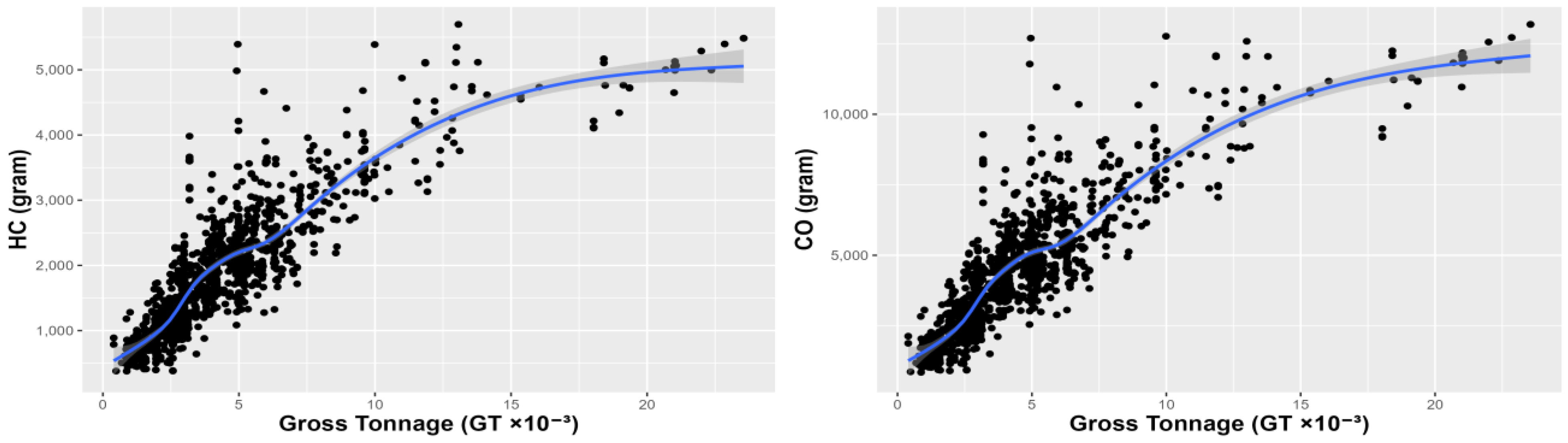
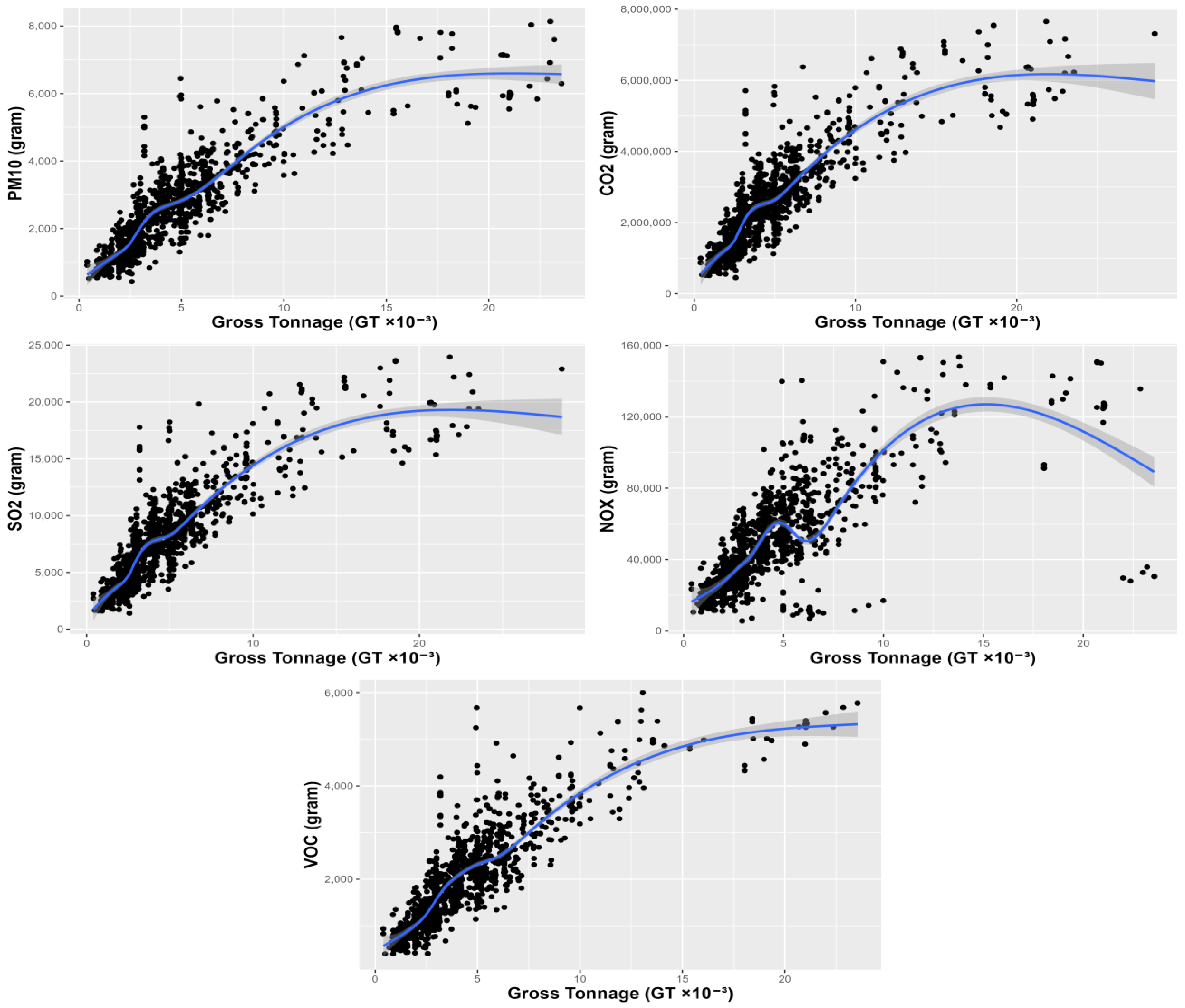
3. Results and Discussion

This section presents the findings from the study, focusing on EPA-based bottom-up emission estimates derived from ship transit data and the outcomes of the structured three-step statistical modeling framework. The results are analyzed to provide insights into the relationship between GT and emissions, as well as to evaluate the performance of the applied regression models.

3.1. Emissions Estimates

Table 6 presents the emission values from the main and auxiliary engines of different types of ships transiting the Bosphorus in 2021, which are calculated as outlined in the previous section. As Table 6 shows, bulk carrier ships contribute the highest emissions across all emission factors. Specifically, bulk carriers account for 33.71% of HC emissions, 33.89% of CO emissions, 33.14% of PM10 emissions, 32.20% of CO2 emissions, 32.22% of SO2 emissions, 32.63% of NOx emissions, and 33.71% of VOC emissions. In terms of total emissions, bulk carriers are responsible for 32.22%, followed by tankers (29.07%), general cargo ships (19.64%), container ships (15.69%), ro-ro ships (1.74%), other ship types (1.54%), and passenger ships (0.10%).
Table 7 presents the number of transits, including repeated passes, for each ship type, alongside the average total main engine power, auxiliary engine power, and GT. These parameters provide valuable insights into the technical characteristics and capacities of various ship types transiting the Bosphorus that are critical for understanding their contributions to emissions and overall environmental impact. Analyzing the data from Table 6 and Table 7 reveals that, although general cargo ships exhibit a higher frequency of repeated transits compared to bulk carriers, the latter contribute a significantly larger share of total emissions. This disparity is primarily due to the substantially higher average main and auxiliary engine power of bulk carriers.
The raw dataset includes repeated passes, meaning that some ships transited the Bosphorus multiple times on different dates in 2021. To develop a reliable GT-based emissions estimation model, these repeated observations must be removed from the dataset to ensure that the data used for modeling consists of unique ships. This step is essential to prevent over-representation of ships with frequent transits and to maintain the independence of observations, a critical assumption in regression modeling. Table 8 presents the number of unique transits for each ship type after the removal of repeated passes. Additionally, it provides the average age of these unique ships, offering insights into the characteristics of the dataset used for statistical modeling. After establishing the unique dataset, the next step involves implementing the three-step statistical modeling framework.
Although emissions are calculated for all ship types, the methodology uses a single ship type to provide a detailed demonstration and provide a clear and focused explanation. General cargo ships have been selected for this purpose due to their dominance in transit frequency, as they represent the most frequent ship type in the Bosphorus in 2021 with a total of 16,472 recorded passes. The analyses focus on this ship type. After removing repeated transits, Table 8 shows 1697 unique general cargo ships with distinct IMO numbers remaining in the dataset, with an average age of 24.72 years.

3.2. Statistical Modeling Results

3.2.1. Outlier Analysis

Rosner’s test is applied to each emission series, calculated using the bottom-up method for general cargo ships, to ensure model reliability and accuracy. Table 9 presents the descriptive statistics regarding emissions before and after outlier detection, highlighting the impact of this step on refining the dataset for subsequent analysis.
The results in Table 9 demonstrate outlier removal to have notably reduced the mean and standard deviation values for most emissions (e.g., HC, CO), thus indicating a more homogenous dataset. Additionally, the range of emissions as reflected in the minimum and maximum values narrows after outlier detection, with the median remaining relatively stable. This suggests that extreme values have been effectively eliminated without significantly altering the central tendency of the data, thus indicating the outliers to have a disproportionate impact on the variability (e.g., standard deviation) but not on the typical values (e.g., median). This refinement ensures that the dataset better represents the typical emission patterns and is more suitable for robust statistical analysis. For instance, 37 outliers are identified and removed in the case of HC, reducing the mean from 1940 to 1830 and the standard deviation from 1210 to 946. This refinement enhances the dataset’s representativeness of typical emissions patterns, thereby improving the robustness and reliability of subsequent regression modeling and analysis.
Following the outlier analysis, scatter plots with smooth curves fitted by locally estimated scatterplot smoothing (LOESS) are provided to identify potential nonlinear relationships between GT and each emission variable (Figure 2). Upon examining these plots, GT is observed to have a distinct nonlinear relationship with HC, CO, PM10, and VOC emissions. Emission levels initially exhibit a rapid increase, followed by a deceleration in growth as GT increases, eventually reaching a saturation point. In such datasets, the dependent variable increases rapidly when the independent variable is at lower values but slows down as the independent variable reaches a certain threshold. The curve gradually flattens or forms a plateau, indicating the saturation phase where the growth effect diminishes. When such trends are present in the relationship between the dependent and independent variables, nonlinear regression models capable of capturing saturation and decelerating growth (e.g., Weibull, Gompertz, and logistic [3p and 4p] models) effectively represent the relationship. Additionally, flexible regression models such as cubic spline and natural spline capture the nonlinear nature of the curve, providing high model fit while preserving interpretability. HC, CO, PM10, and VOC emissions demonstrate a saturation effect in their relationship with GT that is characterized by an earlier onset and a more pronounced plateau. In contrast, CO2 and SO2 emissions exhibit a more gradual saturation pattern, with the curve flattening through a smoother transition. Such saturation behaviors can be effectively represented using nonlinear regression models (e.g., Weibull, Gompertz, and logistic [3p and 4p] models). Furthermore, the cubic spline and natural spline models are well suited for capturing the nonlinear curvature observed in the data as they particularly excel at modeling plateau regions following saturation. In contrast, NOx emissions exhibit a more complex nonlinear pattern compared to other emissions that are characterized by an initial rise followed by a plateau and subsequent decline at higher GT values. Such data behavior necessitates the use of more flexible regression models capable of capturing both the growth and reduction phases. Therefore, the logistic (4p), Gompertz, and Weibull models, as well as spline-based methods, are the most suitable approaches for accurately modeling NOx emission trends.
Detailed interpretation of the scatter plots demonstrates complex nonlinear associations between GT and the emission variables characterized by varying degrees of saturation and trend patterns. Rather than relying solely on polynomial models commonly applied in the literature (e.g., quadratic [second-order] and cubic [third-order] regression models), more comprehensive understanding of these emission patterns can be achieved by considering regression models capable of capturing these complex nonlinear behaviors. The intricate nonlinear trends observed (e.g., rapid initial increases, saturation phases, and eventual declines) indicate that the models specifically developed to capture such behaviors offer a superior representation of the underlying data structure. Thus, selection of the optimal regression model should be based on both the observed data patterns as well as the statistical performance metrics (e.g., RMSE, MAPE) to ensure both precision and interpretability in emission trend analysis.

3.2.2. Regression Modeling

Table 10, Table 11 and Table 12 summarize the performance of the regression models with various curve shapes for HC, CO, PM10, CO2, SO2, NOx, and VOC emissions. After removing the outliers using Rosner’s test, each emission dataset is randomly split into a training set (80%) and a testing set (20%). Regression models are then fitted to the training data separately for each emission type. To enhance the robustness and generalization ability of the models, 10-fold cross-validation is applied during the training process. This method reduces the risk of overfitting by dividing the training data into subsets, thus enabling the model to be trained and validated on different portions of the data. Performance metrics (i.e., NRMSE, PBIAS, and MAPEdiff) are computed to evaluate the accuracy and reliability of each regression model developed to estimate emissions as a function of GT. Table 10 presents the modeling results for HC, CO, and PM10 emissions; Table 11 summarizes the performance metrics for CO2, SO2, and NOx emissions; and Table 12 displays the metrics for VOC emissions.
The mean ± SD values for NRMSE, MAPEdiff, and PBIAS regarding HC emissions are reported as 0.0997 ± 0.0137, 8.8 × 10⁻⁴ ± 6.44 × 10⁻⁴, and −4.76 × 10⁻⁴ ± 5.18 × 10⁻⁴, respectively, reflecting the central tendency and dispersion of the model performance metrics. Among the evaluated regression models, the natural spline model emerges as the most appropriate choice for estimating HC emissions as a function of GT based on its superior performance across multiple evaluation metrics. It demonstrates the lowest NRMSE of 0.0895, indicating high predictive accuracy relative to the range of observed data. Furthermore, the model’s minimal MAPEdiff highlights consistent predictive performance between the training and testing sets. Additionally, the model exhibits minimal systematic bias, with a PBIAS of approximately 0.02%. These strengths underline its suitability for capturing the underlying relationship in the data. The natural spline model is presented as follows with its estimated parameters. Notably, this model describes the relationship with high statistical significance, as all parameter estimates are significant (p < 0.001).
l n H C = 6.301 + 1.237 × S 1 ( G T ) + 1.805 × S 2 ( G T ) + 2.711 × S 3 ( G T ) + 2.085 × S 4 ( G T )
The mean ± SD values for the NRMSE, MAPEdiff, and PBIAS metrics regarding CO emissions are reported as 0.1043 ± 0.0116, 6.68 × 10⁻⁴ ± 6.48 × 10⁻⁴, and 2.63 × 10⁻³ ± 9.14 × 10⁻⁴, respectively. Among the evaluated regression models for estimating the relationship between CO emissions and GT, the Weibull regression model demonstrates the most balanced performance across multiple performance metrics, making it the most suitable choice for CO. While the cubic spline and natural spline models, respectively, achieved lower NRMSE values of 0.0957 and 0.0959 compared to 0.0984 for the Weibull model, both spline models exhibited slightly higher PBIAS values. In contrast, the Weibull model achieves a lower value, thus reflecting reduced systematic error and better overall reliability in the context of this dataset. Additionally, the MAPEdiff values further support the selection of the Weibull model, indicating consistent performance between the training and test datasets. The balance among predictive accuracy (NRMSE), low bias (PBIAS), and consistency (MAPEdiff) highlights the Weibull model’s robustness for capturing the underlying relationship between CO emissions and GT. Considering these results, the Weibull regression model has been selected as the optimal choice due to its superior balance of predictive accuracy, reduced systematic error, and reliable generalization across datasets. The mathematical form of the Weibull regression model is given below along with the estimated parameters. The results also confirm that its statistical significance is worth mentioning, as all parameter estimates are statistically significant (p < 0.001).
l n C O = 9.417 2.859 × e x p ( e x p 6.798 × G T 0.811 )
The mean ± SD values of the performance metrics for PM10 emissions (i.e., NRMSE, MAPEdiff, and PBIAS) are presented as 0.1028 ± 0.0115, 7.86 × 10⁻⁴ ± 3.65 × 10⁻⁴, and 8.26 × 10⁻⁴ ± 9.6 × 10⁻⁴, respectively. Of the evaluated regression models, the cubic spline model demonstrates the best overall performance for predicting PM10 emissions as a function of GT. It achieved the lowest NRMSE (0.0954), thus indicating superior predictive accuracy compared to the other models. Additionally, it maintained a competitive MAPEdiff and exhibited a low PBIAS (0.0014%), thus reflecting minimal systematic bias. The natural spline model also performed well with similar accuracy metrics but presented a slightly higher PBIAS (0.0015%). Also, while the logarithmic model demonstrated the smallest MAPEdiff, indicating high consistency, its higher PBIAS value limits its overall suitability. Simpler models (e.g., linear and quadratic regression) showed higher NRMSE values, indicating less precise predictions for PM10 emissions. Based on these findings, the cubic spline model emerges as a highly suitable choice for modeling PM10 emissions by effectively balancing predictive accuracy, low systematic bias, and consistent performance. The intercept and five out of six spline terms were statistically significant (p < 0.001), thus demonstrating their strong contribution to explaining PM10 variations. Although the first spline term was statistically non-significant (p = 0.498), it was retained to ensure the smoothness and structural integrity of the spline curve, which remains standard practice in regression modeling. The estimated cubic spline model can be mathematically represented as follows, with S1(GT), S2(GT), …, S6(GT) being the basis spline terms corresponding to GT and calculated using degree = 3 with knots placed at the 25th, 50th, and 75th percentiles of GT.
l n P M 10 = 6.615 + 0.112 × S 1 G T + 0.583 × S 2 G T + 1.221 × S 3 G T + 1.981 × S 4 G T + 2.488 × S 5 G T + 2.038 × S 6 ( G T )
The mean ± SD values for the performance metrics of NRMSE, MAPEdiff, and PBIAS regarding CO2 are, respectively, reported as 0.1109 ± 0.0123, 6.74 × 10⁻⁴ ± 2.51 × 10⁻⁴, and −8.76 × 10⁻⁵ ± 3.36 × 10⁻⁴, thus representing the models’ accuracy, consistency, and systematic bias. Of the evaluated regression models for CO2 emissions, the cubic spline and natural spline models exhibit the most optimal performance in terms of predictive accuracy and bias minimization. Both models achieve the lowest NRMSE values (0.1036 for cubic spline and 0.1035 for natural spline), thus indicating high accuracy in capturing the relationship between CO2 and GT. The models also exhibit minimal PBIAS, with the natural spline model achieving the lowest bias, closely followed by the cubic spline model, thus reflecting reliable predictions with minimal systematic error. While the cubic spline model also demonstrates competitive accuracy with an NRMSE = 0.1035, its higher PBIAS compared to the spline models indicates slightly greater systematic bias. Therefore, the natural spline model emerges as the most balanced choice for CO2 as it effectively balances low prediction error and minimal bias, thus making it a robust and interpretable solution. All coefficients (i.e., intercept, natural spline terms) have p < 0.001, indicating strong statistical significance, with each term contributing meaningfully to explaining the variation in CO2 emissions. The estimated natural spline model can be mathematically expressed as follows:
l n C O 2 = 13.345 + 1.324 × S 1 ( G T ) + 2.082 × S 2 G T + 2.958 × S 3 G T + 1.946 × S 4 G T
The mean ± SD values of the performance metrics for NRMSE, MAPEdiff, and PBIAS regarding SO2 are reported as 0.1056 ± 0.0129, 1.45 × 10⁻⁴ ± 1.76 × 10⁻⁴, and 1.41 × 10⁻³ ± 9.5 × 10⁻⁴. Based on the results from modeling SO2 emissions, the natural spline regression model demonstrates superior performance in terms of predictive accuracy and minimal systematic bias. It achieves the lowest NRMSE (0.0962) and the smallest MAPEdiff (9.51 × 10⁻⁶), thus indicating exceptional consistency between the training and testing datasets. Furthermore, it has a minimal PBIAS (0.00194), reflecting negligible systematic error. The cubic spline model closely follows, with a slightly higher NRMSE and comparable error metrics (MAPEdiff = 1.16 × 10⁻⁵; PBIAS = 0.0019). While both models perform exceptionally well, the natural spline model offers marginally better consistency and lower error values. Despite these minor differences, both spline models outperformed other nonlinear regressions (e.g., Weibull, Gompertz, and logistic models), which exhibited notably higher NRMSE values and greater bias, making them less favorable choices. Consequently, the natural spline model provides the most balanced and reliable performance by combining high predictive accuracy with minimal bias and error variation, thus making it the most suitable choice for modeling SO2 emissions. All coefficients (i.e., intercept, natural spline terms) are significant (p < 0.001), thus indicating that each term significantly contributes to explaining the variation in SO2 emissions. The estimated natural spline model can be mathematically expressed as follows:
l n S O 2 = 7.603 + 1.289 × S 1 G T + 2.093 × S 2 G T + 2.953 × S 3 G T + 1.899 × S 4 G T
The mean ± SD values for the NRMSE, MAPEdiff, and PBIAS metrics regarding NOx emissions are reported as 0.1554 ± 0.0071, 1.55 × 10⁻³ ± 4.65 × 10⁻⁴, and −1.12 × 10⁻³ ± 4.23 × 10⁻⁴, respectively. Based on the results obtained from comparing the regression models constructed for NOx emissions, the cubic spline model demonstrates slightly superior overall performance in terms of predictive accuracy and minimal bias. It achieves the lowest NRMSE (0.1469) and smallest MAPEdiff (0.00132), thus indicating high consistency between the training and testing sets. Additionally, it exhibits the lowest PBIAS value, thus reflecting minimal systematic error. The natural spline model also shows competitive performance with a slightly higher NRMSE (0.1501) and a marginally greater PBIAS, suggesting similarly reliable predictive performance. Despite the minimal differences between these two spline models, the cubic spline model slightly outperforms the natural spline in terms of both error magnitude and consistency. Other nonlinear regression models (e.g., Weibull, Gompertz, logistic models) exhibited slightly higher NRMSE and PBIAS values, indicating lower predictive accuracy and marginally increased systematic error compared to the spline models. However, the differences among these models remain moderate, thus suggesting that multiple regression techniques can still provide reasonable approximations for the relationship between NOx emissions and GT. Considering its superior performance across all evaluation metrics (i.e., the lowest NRMSE, minimal PBIAS, and consistent MAPEdiff), the cubic spline model can be identified as the most balanced and reliable approach for modeling the relationship between GT and NOx emissions. All coefficients (i.e., intercept, spline basis terms), are statistically significant (p-values < 0.001), indicating their substantial contribution to explaining the variation in NOx emissions. The estimated cubic spline model can be mathematically expressed as follows, where S1(GT), S2(GT),…, S6(GT) are basis spline terms for GT, calculated using degree = 3 with knots placed at the 25th, 50th, and 75th percentiles of the GT distribution.
l n N O x = 9.652 + 0.378 × S 1 G T + 0.461 × S 2 G T + 1.255 × S 3 G T + 0.568 × S 4 G T + 4.667 × S 5 G T + 0.642 × S 6 G T
The mean ± SD values regarding the VOC emissions models (Table 12) are reported for NRMSE, MAPEdiff, and PBIAS, respectively, as 0.0994 ± 0.01, 4.22 × 10⁻⁴ ± 2.85 × 10⁻⁴, and −2.37 × 10⁻³ ± 8.58 × 10⁻⁴, reflecting the models’ predictive accuracy, consistency, and systematic bias. Based on its performance metrics, the cubic spline model demonstrates the most superior overall performance among the evaluated regression models for VOC emissions modeling. It achieves the lowest NRMSE (0.09196) and a minimal MAPEdiff, thus highlighting strong predictive accuracy and consistency between the training and testing datasets. Additionally, its low PBIAS further indicates minimal systematic error, supporting its reliability for capturing the relationship between VOC emissions and GT. The natural spline model also performs competitively, with a similarly low NRMSE and MAPEdiff. However, it exhibited a slightly higher PBIAS, indicating a marginally greater systematic error compared to the cubic spline model. The other models (e.g., Weibull, Gompertz) achieved competitive NRMSE values but showed higher PBIAS and MAPEdiff values, making them less favorable for this dataset. Simpler models such as linear and exponential growth regressions demonstrated higher error rates and greater systematic bias, further limiting their suitability. The cubic spline model emerges as the most balanced and reliable option by combining minimal error, high predictive accuracy, and low bias, thus making it the optimal choice among the considered models. The p values for all spline basis terms except the first term (S1) are less than 0.001, confirming their statistical significance. Although the first basis spline term (p = 0.574) exceeds the conventional significance threshold, it has been kept in the model to maintain the structural integrity and smoothness of the cubic spline framework. The overall model fit remains strong, with the remaining significant spline terms effectively capturing the nonlinear relationship between VOC emissions and GT. The estimated cubic spline model can be mathematically expressed as follows, where S1(GT), S2(GT), …, S6(GT) are basis spline terms corresponding to GT and calculated using degree = 3 with knots placed at the 25th, 50th, and 75th percentiles of GT:
l n V O C = 6.434 + 0.090 × S 1 G T + 0.496 × S 2 G T + 1.168 × S 3 G T + 1.864 × S 4 G T + 2.401 × S 5 G T + 2.029 × S 6 G T
The findings from this study emphasize the importance of evaluating multiple regression models to accurately capture the nonlinear relationships between gross tonnage (GT) and various emission types. By applying a comprehensive statistical modeling framework, seven emission types (HC, CO, PM10, CO2, SO2, NOx, and VOC) have been systematically analyzed using a diverse set of 12 regression models. Key performance metrics (i.e., NRMSE, MAPEdiff, and PBIAS) were employed to assess the models’ predictive accuracy, consistency, and systematic bias. The results indicate the natural spline model to provide the most reliable estimations for HC, SO2, and CO2 emissions, while the Weibull regression model demonstrated superior performance for CO emissions. For PM10, NOx, and VOC emissions, the cubic spline model outperformed the other models in terms of error reduction and generalization ability.
Overall, the comparative analysis of the regression models across all seven emission types reveals that spline-based models, particularly the natural spline and cubic spline regressions, consistently deliver superior performance in terms of predictive accuracy, minimal bias, and generalization ability. The natural spline model has demonstrated the most reliable results for HC, SO2, and CO2 emissions, effectively balancing low error metrics and reduced systematic bias. Similarly, the cubic spline model provides the best fit for PM10, NOx, and VOC emissions, with consistently low NRMSE and minimal bias across training and testing datasets. Meanwhile, the Weibull regression model has emerged as the most suitable for CO emissions due to its ability to maintain low bias while achieving competitive error metrics. These results suggest that flexible, nonlinear regression models, particularly those capable of adapting to complex data structures such as splines, are more effective at capturing the nonlinear relationships between GT and emissions compared to simpler polynomial models.

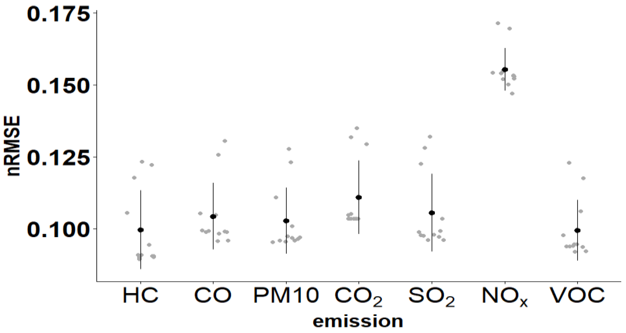
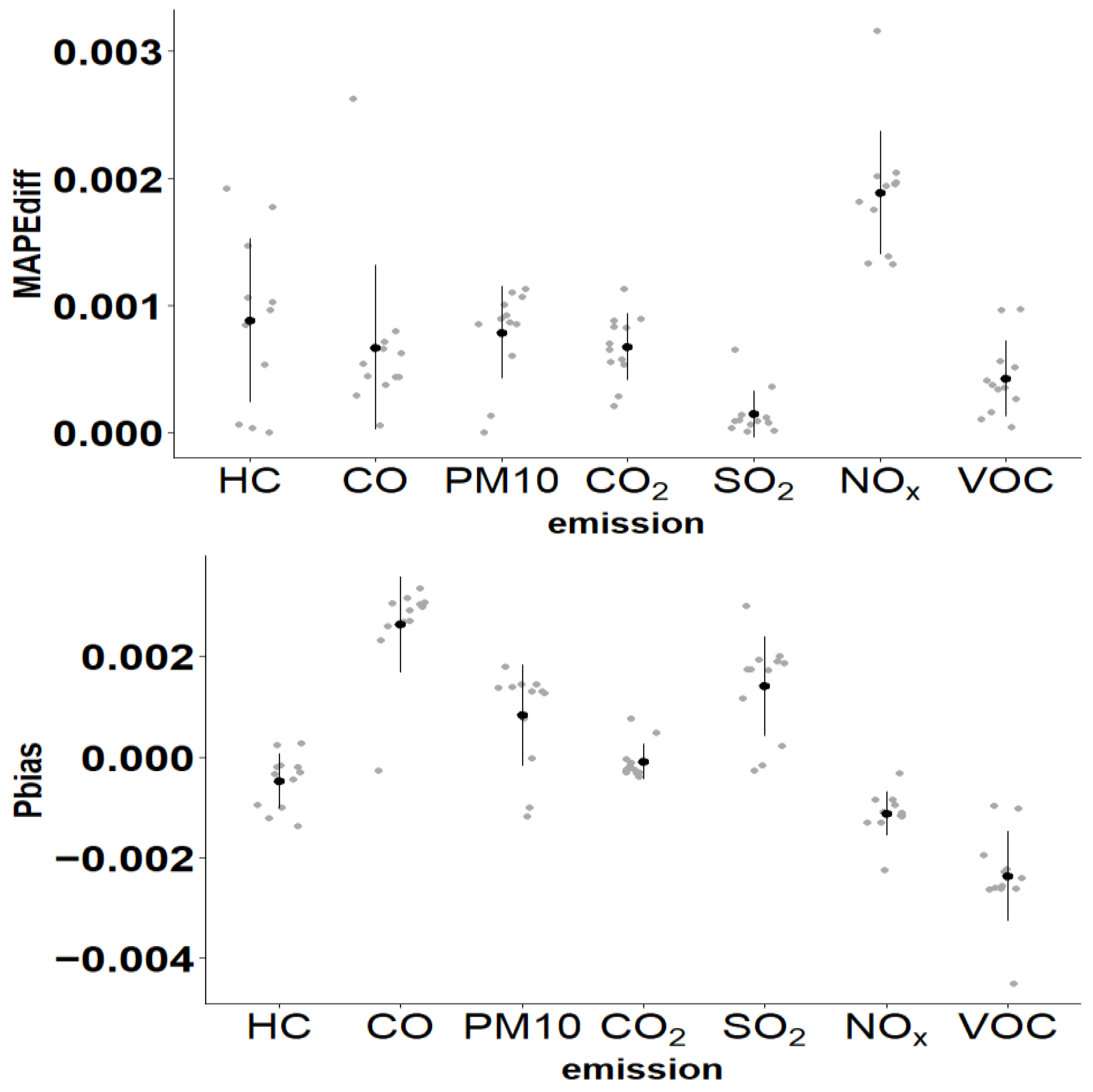
3.2.3. Performance Comparison Metrics

The NRMSE and PBIAS plots (Figure 3) reveal that most regression models yielded closely aligned results with minimal variability across emissions. However, the variability in MAPEdiff values across models was more pronounced, indicating greater dispersion regarding the absolute percentage errors among the models. As reflected by error variability, this suggests that considering not only predictive accuracy (e.g., NRMSE, PBIAS) but also the consistency and generalization ability of the models are essential when comparing and selecting the best-fitting regression model.

4. Conclusions

The continued growth of maritime trade, which constitutes the vast majority of global trade volume, has raised mounting concerns over ship-based emissions and their environmental consequences. In response, international regulatory frameworks—particularly those established by the IMO—have introduced strategies such as the EEXI and CII to curb pollutants like NOx, SOx, PM, and CO2, which are closely linked to air quality degradation, ecological harm, and public health risks. Among high-traffic maritime corridors, the Bosphorus stands out due to its ecological sensitivity and close proximity to densely populated areas. In this context, adopting data-driven approaches to emission estimation is essential for supporting sustainable maritime operations and informing effective mitigation strategies.
In line with this objective, this study employs a bottom-up approach to estimate HC, CO, PM10, CO2, SO2, NOx, and VOC emissions from various ship types (i.e., bulk carriers, container ships, general cargo vessels, passenger ships, ro-ro vessels, tankers, and others) transiting the Bosphorus in 2021. These emissions are calculated for each of the 38,304 vessel transits based on ship-specific operational characteristics, using standardized formulas defined in the U.S. EPA methodology. The results show that bulk carriers account for 32.22% of total emissions, followed by tankers (29.07%) and general cargo vessels (19.64%). In contrast, passenger ships, ro-ro vessels, and other ship types contribute much smaller shares, accounting for 0.10%, 1.74%, and 1.54% of total emissions, respectively.
Following the emissions estimation process, the analysis focuses on general cargo vessels, which are selected as a representative case for detailed modeling. This decision is based on the fact that general cargo vessels accounted for 43% of all ship transits in the Bosphorus in 2021, making them the most frequently transiting vessel type and enabling a more targeted exploration of GT–emission relationships within a consistent vessel category. To avoid potential bias caused by repeated passages of the same vessel, the dataset is filtered to retain only unique ships based on their IMO identification numbers. This step ensures that each observation used in the modeling process corresponds to a distinct vessel, thereby preventing overrepresentation of frequently transiting ships and improving the validity of the regression analysis. Building on this refined dataset, a three-step statistical modeling framework is implemented, with GT used as the primary predictor variable. A critical component of the first step involves handling outliers, as their presence can disproportionately influence error metrics, thus potentially leading to misleading model evaluation results. Given that outliers can significantly affect the comparative assessment of regression models by distorting performance measures, their identification and removal remain essential for ensuring accurate and unbiased model comparisons [43]. As a result, the first step involves detecting outliers using Rosner’s test, ensuring a refined dataset that enhances the accuracy and stability of subsequent modeling phases. The second step involves fitting 12 regression models—categorized into polynomial, concave/convex, sigmoidal, and spline curve types—to explore both linear and nonlinear relationships between GT and each emission factor. Splitting the dataset into training (80%) and testing (20%) subsets, the modeling phase is further strengthened by implementing a 10-fold cross-validation to ensure robust error assessment across different data partitions. In the third and final step, the performance of each model is evaluated using multiple error metrics, including NRMSE, MAPEdiff, and PBIAS, to comprehensively assess predictive accuracy, consistency, and bias. This structured approach not only enables the identification of the most suitable model for each emission type but also enhances the overall robustness of emission predictions within maritime applications.
The results demonstrate that nonlinear regression models provide a superior fit compared to simpler polynomial models. In particular, spline-based models—namely, natural spline and cubic spline—outperform other approaches for most emission types (i.e., HC, PM10, SO2, and VOC) due to their flexibility in capturing complex, nonlinear relationships. The Weibull regression model also stands out as a top performer, especially for CO and NOx emissions, offering a balance between predictive accuracy and minimal systematic bias. These findings underscore the value of employing flexible regression techniques, such as spline-based models, to more effectively capture intricate emission patterns and improve the accuracy of ship-based emission estimations, reinforcing the methodological contribution outlined earlier.
In summary, this study introduces a structured and comparative three-step statistical modeling framework, developed on the basis of ship-based emissions first estimated using a bottom-up approach. The framework emphasizes the value of testing a broad spectrum of regression forms to better capture complex, nonlinear relationships between gross tonnage and emissions. Notably, the simultaneous application of a diverse range of nonlinear regression models—including spline-based techniques—offers a distinctive contribution to maritime emission modeling, where such comprehensive comparisons, especially those involving splines, have remained relatively limited. The observed variation in model performance across different emissions highlights the importance of adopting pollutant-specific modeling strategies tailored to the characteristics of each dataset. This structured and replicable approach enhances the accuracy and robustness of emissions estimation and contributes actionable insights for developing data-driven policies that support more sustainable maritime practices.
For future studies, broadening the scope of emission modeling may enhance both the accuracy and applicability of the proposed framework. This could involve extending the methodology to additional vessel categories beyond general cargo ships (e.g., bulk carriers, tankers, and container vessels) and incorporating ship-specific variables such as operational speed, fuel type, and engine specifications. These refinements would allow for more precise emissions estimations by accounting for a broader range of influencing factors, thereby reducing estimation errors and improving the alignment between predicted and actual emission levels. Furthermore, testing the framework across various maritime regions and operational scenarios would strengthen its validity under various conditions. A more diverse dataset and extended application of the model could support the development of a flexible, data-driven tool for maritime emissions management and policy design, thereby promoting sustainable practices in the shipping industry on a global scale. In addition, future research could explore the integration of ML and AI techniques to further strengthen predictive capabilities, particularly as larger and more diverse datasets become available. While the current study emphasizes interpretability and explanatory power through regression-based modeling, incorporating ML/AI approaches may offer complementary benefits by improving forecasting performance across complex maritime environments.

Funding

This research received no external funding.

Data Availability Statement

The data presented in this article are available upon request from the corresponding author.

Conflicts of Interest

The author declares no conflicts of interest.

Nomenclature

AISAutomatic identification systemIMOInternational maritime organization
aomiscsR package for statistical methods for the agricultural sciencesLOESSLocally weighted smoothing
BSFCBrake specific fuel consumptionMAPEMean absolute percentage error
CaretR package for classification and regression TrainingMDOMarine diesel oil
CH4MethaneMetricsR package for evaluation metrics for machine learning
COCarbon monoxideMSDMedium-speed diesel
CO2Carbon dioxideN2ONitrous oxide
DECADomestic emission control areanlmeR package for nonlinear mixed-effects
drcR package for dose–response curvesNMVOCNon-methane VOC
ECAEmission control areaNOxNitrogen oxides
ENTECEnvironmental engineering consultancyNRMSENormalized root mean squared error
EnvStatsR package for environmental statisticsPBIASPercent bias
EPAEnvironmental protection agencyPM10Particulate matter with an aerodynamic diameter of less than 10 μm
ESDExtreme studentized deviateR2Coefficient of determination
ggplot2R package for data visualization (the grammar of graphics)SO2Sulfur dioxide
GTGross tonnageSOXSulfur oxides
HCHydrocarbonSSDSlow-speed diesel
HFOResidual fuel (heavy fuel oil)VOCVolatile organic compounds
HSDHigh-speed dieselML/AIMachine Learning/Artificial Intelligence

References

  1. Shi, W.; Xiao, Y.; Chen, Z.; McLaughlin, H.; Li, K.X. Evolution of green shipping research: Themes and methods. Marit. Policy Manag. 2018, 45, 863–876. [Google Scholar]
  2. Zincir, B. Slow steaming application for short-sea shipping to comply with the CII regulation. Brodogradnja 2023, 74, 21–38. [Google Scholar]
  3. Wan, Z.; Zhu, M.; Chen, S.; Sperling, D. Pollution: Three steps to a green shipping industry. Nature 2016, 530, 275–277. [Google Scholar]
  4. Eyring, V.; Isaksen, I.S.; Berntsen, T.; Collins, W.J.; Corbett, J.J.; Endresen, O.; Grainger, R.G.; Moldanova, J.; Schlager, H.; Stevenson, D.S. Transport impacts on atmosphere and climate: Shipping. Atmos. Environ. 2010, 44, 4735–4771. [Google Scholar]
  5. Xu, X.; Yang, H.; Li, C. Theoretical model and actual characteristics of air pollution affecting health cost: A review. Int. J. Environ. Res. Public Health 2022, 19, 3532. [Google Scholar] [CrossRef]
  6. Kalajdžić, M.; Vasilev, M.; Momčilović, N. Power reduction considerations for bulk carriers with respect to novel energy efficiency regulations. Brodogradnja 2022, 73, 79–92. [Google Scholar]
  7. Kalajdžić, M.; Vasilev, M.; Momčilović, N. Inland waterway cargo vessel energy efficiency in operation. Brodogradnja 2023, 74, 71–89. [Google Scholar] [CrossRef]
  8. Birpınar, M.E.; Talu, G.F.; Gönençgil, B. Environmental effects of maritime traffic on the Bosphorus. Environ. Monit. Assess. 2009, 152, 13–23. [Google Scholar]
  9. Chen, D.; Zhao, N.; Lang, J.; Zhou, Y.; Wang, X.; Li, Y.; Zhao, Y.; Guo, X. Contribution of ship emissions to the concentration of PM2. 5: A comprehensive study using AIS data and WRF/Chem model in Bohai Rim Region, China. Sci. Total Environ. 2018, 610–611, 1476–1486. [Google Scholar]
  10. Fabregat, A.; Vázquez, L.; Vernet, A. Using Machine Learning to estimate the impact of ports and cruise ship traffic on urban air quality: The case of Barcelona. Environ. Model. Softw. 2021, 139, 104995. [Google Scholar]
  11. Ekmekçioğlu, A.; Ünlügençoğlu, K.; Çelebi, U.B. Estimation of shipping emissions based on real-time data with different methods: A case study of an oceangoing container ship. Environ. Dev. Sustain. 2022, 24, 4451–4470. [Google Scholar]
  12. Nunes, R.A.; Alvim-Ferraz, M.C.; Martins, F.G.; Penuelas, A.L.; Durán-Grados, V.; Moreno-Gutiérrez, J.; Jalkanen, J.P.; Sousa, S.I. Estimating the health and economic burden of shipping related air pollution in the Iberian Peninsula. Environ. Int. 2021, 156, 106763. [Google Scholar] [PubMed]
  13. Viana, M.; Rizza, V.; Tobías, A.; Carr, E.; Corbett, J.; Sofiev, M.; Karanasiou, A.; Buonanno, G.; Fann, N. Estimated health impacts from maritime transport in the Mediterranean region and benefits from the use of cleaner fuels. Environ. Int. 2020, 138, 105670. [Google Scholar] [CrossRef] [PubMed]
  14. Gössling, S.; Meyer-Habighorst, C.; Humpe, A. A global review of marine air pollution policies, their scope and effectiveness. Ocean Coast. Manag. 2021, 212, 105824. [Google Scholar]
  15. Tuswan, T.; Sari, D.P.; Muttaqie, T.; Prabowo, A.R.; Soetardjo, M.; Murwantono, T.T.P.; Ridwan, U.; Yuniati, Y. Representative application of LNG-fuelled ships: A critical overview on potential GHG emission reductions and economic benefits. Brodogradnja 2023, 74, 63–83. [Google Scholar] [CrossRef]
  16. Ekmekçioğlu, A.; Kuzu, S.L.; Ünlügençoğlu, K.; Çelebi, U.B. Assessment of shipping emission factors through monitoring and modelling studies. Sci. Total Environ. 2020, 743, 140742. [Google Scholar]
  17. Yang, L.; Zhang, Q.; Lv, Z.; Zhang, Y.; Yang, Z.; Fu, F.; Wu, L.; Mao, H. Efficiency of DECA on ship emission and urban air quality: A case study of China port. J. Clean. Prod. 2022, 362, 132556. [Google Scholar] [CrossRef]
  18. Toscano, D.; Murena, F.; Quaranta, F.; Mocerino, L. Assessment of the impact of ship emissions on air quality based on a complete annual emission inventory using AIS data for the port of Naples. Ocean Eng. 2021, 232, 109166. [Google Scholar] [CrossRef]
  19. Kuzu, S.L.; Bilgili, L.; Kiliç, A. Estimation and dispersion analysis of shipping emissions in Bandirma Port, Turkey. Environ. Dev. Sustain. 2021, 23, 10288–10308. [Google Scholar]
  20. Kanberoğlu, B.; Kökkülünk, G. Assessment of CO2 emissions for a bulk carrier fleet. J. Clean. Prod. 2021, 283, 124590. [Google Scholar] [CrossRef]
  21. Kılıç, A.; Yolcu, M.; Kılıç, F.; Bilgili, L. Assessment of ship emissions through cold ironing method for Iskenderun Port of Turkey. Environ. Res. Technol. 2020, 3, 193–201. [Google Scholar]
  22. Endresen, Ø.; Sørgård, E.; Behrens, H.L.; Brett, P.O.; Isaksen, I.S. A historical reconstruction of ships’ fuel consumption and emissions. J. Geophys. Res. Atmos. 2007, 112, 1–17. [Google Scholar]
  23. Bilgili, L.; Celebi, U.B. Developing a new green ship approach for flue gas emission estimation of bulk carriers. Measurement 2018, 120, 121–127. [Google Scholar]
  24. Ekmekçioğlu, A.; Ünlügençoğlu, K.; Çelebi, U.B. Container ship emission estimation model for the concept of green port in Turkey. Proc. Inst. Mech. Eng. Part M J. Eng. Marit. Environ. 2022, 236, 504–518. [Google Scholar]
  25. Chen, D.; Wang, X.; Li, Y.; Lang, J.; Zhou, Y.; Guo, X.; Zhao, Y. High-spatiotemporal-resolution ship emission inventory of China based on AIS data in 2014. Sci. Total Environ. 2017, 609, 776–787. [Google Scholar]
  26. Peng, X.; Wen, Y.; Wu, L.; Xiao, C.; Zhou, C.; Han, D. A sampling method for calculating regional ship emission inventories. Transp. Res. Part D Transp. Environ. 2020, 89, 102617. [Google Scholar]
  27. Gunes, U. Estimating bulk carriers’ main engine power and emissions. Brodogradnja 2023, 74, 85–98. [Google Scholar]
  28. Ozsari, I. Predicting main engine power and emissions for container, cargo, and tanker ships with artificial neural network analysis. Brodogradnja 2023, 74, 77–94. [Google Scholar]
  29. Trozzi, C. Emission Estimate Methodology for Maritime Navigation; EPA: Rome, Italy, 2010. [Google Scholar]
  30. Álvarez, P.S. From maritime salvage to IMO 2020 strategy: Two actions to protect the environment. Mar. Pollut. Bull. 2021, 170, 112590. [Google Scholar]
  31. Hastie, T.; Tibshirani, R.; Friedman, J. The Elements of Statistical Learning: Data Mining, Inference, and Prediction, 2nd ed.; Springer: Berlin/Heidelberg, Germany, 2009. [Google Scholar]
  32. R: A Language and Environment for Statistical Computing. R Foundation for Statistical Computing, 2021. The R Project. Available online: https://www.R-project.org/ (accessed on 1 June 2023).
  33. Ay, C.; Seyhan, A.; Beşikçi, E.B. Quantifying ship-borne emissions in Bosphorus with bottom-up and machine-learning approaches. Ocean Eng. 2022, 258, 111864. [Google Scholar]
  34. Methodologies for Estimating Port-Related and Goods Movement Mobile Source Emission Inventories, 2020. EPA—Office of Transportation Air Quality. Available online: https://nepis.epa.gov/Exe/ZyPURL.cgi?Dockey=P100YFY8.TXT (accessed on 1 June 2023).
  35. Rosner, B. Percentage points for a generalized ESD many-outlier procedure. Technometrics 1983, 25, 165–172. [Google Scholar]
  36. Cudeck, R.; Toit, S.H.D. A version of quadratic regression with interpretable parameters. Multivar. Behav. Res. 2002, 37, 501–519. [Google Scholar]
  37. Ratkowsky, D.A. Principles of nonlinear regression modeling. J. Ind. Microbiol. 1993, 12, 195–199. [Google Scholar]
  38. Crawley, M.J. The R book; John Wiley & Sons: Hoboken, NJ, USA, 2012. [Google Scholar]
  39. Freund, R.J.; Wilson, W.J.; Sa, P. Regression Analysis; Elsevier: Amsterdam, The Netherlands, 2006. [Google Scholar]
  40. Fox, J.; Weisberg, S. Nonlinear Regression, Nonlinear Least Squares, and Nonlinear Mixed Models in R. Population; McMaster: Hamilton, ON, Canada, 2019. [Google Scholar]
  41. Huang, H.-H.; He, Q. Nonlinear Regression Analysis; Elsevier: Amsterdam, The Netherlands, 2023. [Google Scholar]
  42. Marquardt, D.W. An algorithm for least-squares estimation of nonlinear parameters. J. Soc. Ind. Appl. Math. 1963, 11, 431–441. [Google Scholar]
  43. Baty, F.; Ritz, C.; Charles, S.; Brutsche, M.; Flandrois, J.P.; Delignette-Muller, M.L. A toolbox for nonlinear regression in R: The package nlstools. J. Stat. Softw. 2015, 66, 1–21. [Google Scholar]
  44. Archontoulis, S.V.; Miguez, F.E. Nonlinear regression models and applications in agricultural research. Agron. J. 2015, 107, 786–798. [Google Scholar]
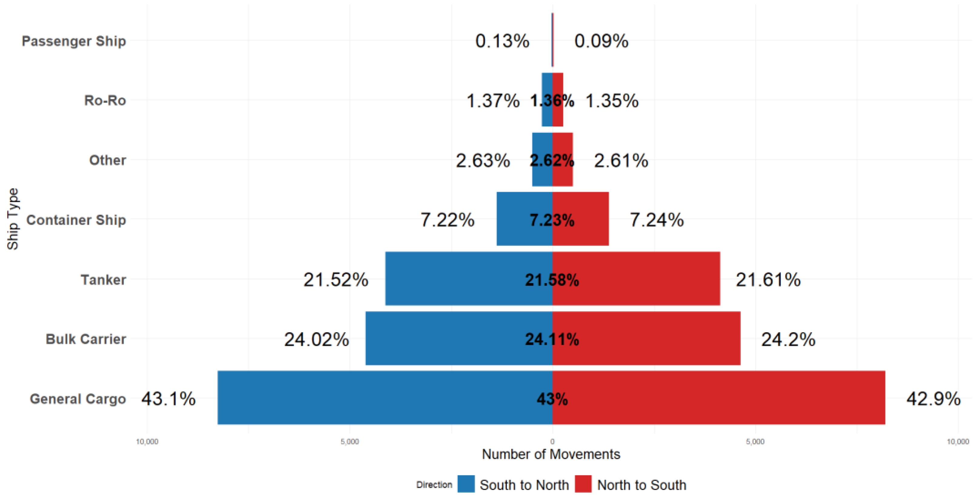
Figure 1. Transit distributions by ship type.
Jmse 13 00744 g001
Figure 2. LOESS-fitted smooth curves showing the relationship between GT and emissions for general cargo ships.
Jmse 13 00744 g002aJmse 13 00744 g002b
Figure 3. Error bars of performance metrics.
Jmse 13 00744 g003aJmse 13 00744 g003b
Table 1. Distribution of ship movements in the Bosphorus by vessel type and traffic direction.
Ship TypeS-NN-STotal
Bulk Carrier462946069235
Container Ship138513842769
General Cargo8208826416,472
Passenger Ship182442
Ro-Ro259263522
Tanker413441268260
Other4995051004
Total19,13219,17238,304
Table 2. Vessel HC and CO emissions (g/kWh) [34].
Engine GroupEngine TypeHC Emissions (g/kWh)CO Emissions (g/kWh)
PropulsionSSD0.61.4
MSD0.51.1
AuxiliaryMSD0.41.1
HSD0.40.9
SSD is engine speed ≤ 300 rpm; MSD is engine speed between 300 and 900 rpm; HSD is engine speed ≥ 900 rpm.
Table 3. Vessel BSFC rates (g/kWh) [34].
Engine GroupFuel TypeEngine TypeBSFC (g/kWh)
PropulsionMDOSSD185
MSD205
HFOSSD195
MSD215
AuxiliaryMDOMSD217
HSD217
HFOMSD227
HSD227
Table 4. Vessel EF(NOx) in g/kWh [34].
Engine GroupFuel TypeNOx TierEngine TypeEF (g/kWh)
PropulsionMDO<1999SSD17
MSD13.2
Tier ISSD16
MSD12.2
Tier IISSD14.4
MSD10.5
Tier IIISSD3.4
MSD2.6
HFO<1999SSD18.1
MSD14
Tier ISSD17
MSD13
Tier IISSD15.3
MSD11.2
Tier IIISSD3.4
MSD2.6
AuxiliaryMDO<1999MSD10.9
HSD13.8
Tier IMSD9.8
HSD12.2
Tier IIMSD7.7
HSD10.5
Tier IIIMSD2
HSD2.6
HFO<1999MSD14.7
HSD11.6
Tier IMSD13
HSD10.4
Tier IIMSD11.2
HSD8.2
Tier IIIMSD2
HSD2.6
Table 5. Mathematical functions and parameter descriptions of the regression models [39,40,41].
Regression ModelMathematical FunctionParameter Descriptions
Linear Regression y = β 0 + β 1 x β 0 = intercept; β 1 = slope
Quadratic Regression y = β 0 + β 1 x + β 2 x 2 β 0 = intercept; β 1 = linear term; β 2 = quadratic term
Cubic Regression y = β 0 + β 1 x + β 2 x 2 + β 3 x 3 β 0 = intercept; β 1 = linear term; β 2 = quadratic term;
β 3 = cubic term
Exponential Regression y = β 0 e x p β 1 x β 0 = scaling parameter; β 1 = growth rate
Logarithmic Regression y = β 0 + β 1 l o g ( X ) β 0 = intercept; β 1 = growth rate
Rectangular Hyperbola Regression y = β 1 X / β 2 + X β 1 = upper asymptote; β 2 = affinity parameter
Three-parameter Logistic Regression y = β 1 1 + e x p β 2 X / β 3 β 1 = upper asymptote; β 2 = inflection point;
β 3 = growth rate
Four-parameter Logistic Regression y = β 4 + β 1 β 4 1 + e x p β 2 X / β 3 β 1 = upper asymptote; β 2 = inflection point;
β 3 = growth rate; β 4 = lower asymptote
Gompertz Regression y = β 1 e x p β 2 β 3 X β 1 = asymptote; β 2 = zero-response parameter;
β 3 = growth rate
Weibull Regression y = β 1 β 2 e x p e x p β 3 x β 4 β 1 = lower asymptote; β 2 = scaling parameter;
β 3
= logarithmic rate parameter; β 4 = shape parameter
Cubic Spline Regression y = β 0 + j = 1 k γ j S j x where
S j x = x κ j 3 i f   x > κ j 0 i f   x κ j
β 0 = intercept; γ = spline coefficient (knot coefficient); S j x = spline basis function; κ = knot points
Natural Spline Regression y = β 0 + j = 1 k γ j S j x where
S j x = x κ j + 3 x κ k 1 + 3 κ k κ j κ k κ k 1
β 0 = intercept; γ = spline coefficient (knot coefficient); S j x = spline basis function; κ = knot points
Table 6. Ship emission estimates for the Bosphorus—EPA (ton.y−1).
Ship TypeHCCOPM10CO2SO2NOxVOCTOTAL
Bulk Carrier
(%)
54.29
(33.71%)
127.86
(33.89%)
65.06
(33.14%)
57,792.75
(32.20%)
180.9
(32.22%)
1308.05
(32.63%)
57.17
(33.71%)
59,586.08
(32.22%)
Container Ship
(%)
25.86
(16.06%)
60.81
(16.12%)
31.25
(15.92%)
28,080.48
(15.65%)
87.88
(15.65%)
706.28
(17.62%)
27.23
(16.06%)
29,019.79
(15.69%)
General Cargo
(%)
28.5
(17.70%)
65.83
(17.45%)
37.3
(19.00%)
35,299.39
(19.67%)
110.38
(19.66%)
762.11
(19.01%)
30.01
(17.70%)
36,333.52
(19.64%)
Other
(%)
2.17
(1.35%)
5
(1.33%)
1.34
(0.68%)
2778.22
(1.55%)
8.47
(1.51%)
49.91
(1.24%)
2.29
(1.35%)
2847.4
(1.54%)
Passenger Ship
(%)
0.14
(0.09%)
0.31
(0.08%)
0.19
(0.10%)
181.42
(0.10%)
0.57
(0.10%)
3.63
(0.09%)
0.14
(0.08%)
186.4
(0.10%)
Ro-Ro
(%)
2.5
(1.55%)
5.79
(1.53%)
3.24
(1.65%)
3125.06
(1.74%)
9.76
(1.74%)
69.48
(1.73%)
2.63
(1.55%)
3218.46
(1.74%)
Tanker
(%)
47.58
(29.55%)
111.72
(29.61%)
57.92
(29.51%)
52,227.91
(29.10%)
163.43
(29.11%)
1109.42
(27.67%)
50.1
(29.55%)
53,768.08
(29.07%)
Total161.04377.32196.3179,485.23561.394008.88169.57184,959.7
Table 7. Technical characteristics and transit frequencies of ship types.
Ship TypeNumber of Multiple TransitsAverage of Total Main Engine (KW)Average of Total Auxiliary Engine (KW)Average GT
Bulk Carrier92357731.05610.3629,155.43
Container Ship276918,286.911383.1223,298.96
General Cargo16,4722068.85246.204057.81
Other10042773.56417.863133.79
Passenger Ship425881.62393.747545.71
Ro-Ro5228566.141149.3421,310.17
Tanker82607583.78708.3926,197.48
Table 8. Summary of unique ship transits by type.
Ship TypeNumber of Unrepeated PassesAverage Age (Years)
Bulk Carrier242811.03
Container Ship22918.23
General Cargo169724.72
Other19524.01
Passenger Ship1435.21
Ro-Ro5326.53
Tanker145511.52
Table 9. Descriptive statistics of emissions for general cargo ships before and after outlier detection.
EmissionBefore Outlier RemovalAfter Outlier Removal
HC A
Overalln = 1697n = 1660
Mean (SD)1940 (1210)1830 (946)
Median [Min, Max]1670 [378, 13,800]1630 [378, 5700]
CO B
Overalln = 1697n = 1659
Mean (SD)4480 (2850)4210 (2190)
Median [Min, Max]3780 [849, 32,900]3720 [849, 13,200]
PM10 C
Overalln = 1697n = 1687
Mean (SD)2560 (1500)2510 (1370)
Median [Min, Max]2250 [427, 16,200]2250 [427, 8130]
CO2 D
Overalln = 1697n = 1691
Mean (SD)2,420,000 (1,380,000)2,390,000 (1,290,000)
Median [Min, Max]2150,000 [450,000, 15,100,000]2,140,000 [450,000, 7,660,000]
SO2 E
Overalln = 1697n = 1691
Mean (SD)7560 (4300)7470 (4040)
Median [Min, Max]6750 [1400, 47,100]6690 [1400, 24,000]
NOx F
Overalln = 1697n = 1667
Mean (SD)50,200 (33,500)47,500 (26,600)
Median [Min, Max]41,400 [5590, 413,000]40,800 [5590, 154,000]
VOC G
Overalln = 1697n = 1660
Mean (SD)2050 (1280)1930 (996)
Median [Min, Max]1760 [398, 14,600]1720 [398, 6000]
Descriptions A: In accordance with Rosner’s test, 37 outliers have been detected and removed. B: In accordance with Rosner’s test, 38 outliers have been detected and removed. C: In accordance with Rosner’s test, 10 outliers have been detected and removed. D: In accordance with Rosner’s test, 6 outliers have been detected and removed. E: In accordance with Rosner’s test, 6 outliers have been detected and removed. F: In accordance with Rosner’s test, 30 outliers have been detected and removed. G: In accordance with Rosner’s test, 37 outliers have been detected and removed.
Table 10. HC, CO, and PM10 modeling results.
HCCOPM10
Regression ModelsNRMSEMAPEdiffPBIASNRMSEMAPEdiffPBIASNRMSEMAPEdiffPBIAS
Linear0.11780.00010.00120.12580.00070.00270.12310.00090.0010
Quadratic0.09450.00050.00040.10480.00010.00270.10100.00060.0000
Cubic0.09100.00080.00030.09940.00030.00230.09730.00100.0008
Exponential0.12230.00000.00140.13060.00080.00330.12770.00090.0012
Logarithmic0.09060.00100.00030.09890.00050.00260.09590.00010.0014
Rect. Hyp.0.10550.00190.00100.10540.00260.00030.11090.00020.0018
Logistic (3p)0.09100.00090.00020.09920.00040.00310.09700.00110.0013
Logistic (4p)0.09050.00100.00020.09880.00040.00300.09650.00110.0013
Gompertz0.12340.00000.00100.09900.00040.00300.09680.00110.0013
Weibull0.09000.00110.00020.09840.00040.00290.09590.00090.0014
Cubic Spline0.09010.00180.00030.09570.00070.00320.09540.00090.0014
Natural Spline0.08950.00150.00020.09590.00060.00310.09550.00090.0015
Table 11. CO2, SO2, and NOx modeling results.
CO2SO2NOx
Regression ModelsNRMSEMAPEdiffPBIASNRMSEMAPEdiffPBIASNRMSEMAPEdiffPBIAS
Linear Reg0.12940.00090.00050.12810.00010.00030.16960.00140.0010
Quadratic Reg0.10510.00020.00020.10340.00040.00020.15420.00180.0013
Cubic Reg0.10350.00030.00020.09890.00000.00120.15410.00180.0013
Exponential Reg0.13180.00090.00080.13200.00010.00020.17150.00130.0008
Logarithmic Reg0.10480.00070.00000.09930.00010.00200.15220.00200.0011
Rect. Hyp. Reg0.13490.00110.00040.12270.00070.00300.15480.00320.0022
Logistic (3p) Reg0.10360.00050.00030.09790.00010.00170.15330.00200.0012
Logistic (4p) Reg0.10350.00060.00030.09760.00010.00170.15290.00200.0012
Gompertz Reg0.10360.00060.00030.09770.00010.00180.15310.00200.0012
Weibull Reg0.10360.00070.00030.09720.00010.00190.15210.00200.0011
Cubic Spline0.10360.00080.00010.09620.00000.00190.14690.00130.0003
Natural Spline0.10350.00080.00010.09620.00000.00190.15010.00190.0009
Table 12. VOC modeling results.
VOC
Regression ModelsNRMSEMAPEdiffPBIAS
Linear0.11750.00030.0010
Quadratic0.09790.00010.0019
Cubic0.09460.00040.0022
Exponential0.12300.00020.0010
Logarithmic0.09460.00060.0026
Rect. Hyp.0.10610.00000.0045
Logistic (3p)0.09410.00030.0026
Logistic (4p)0.09390.00040.0026
Gompertz0.09400.00040.0026
Weibull0.09360.00050.0026
Cubic Spline0.09200.00100.0023
Natural Spline0.09220.00100.0024
Disclaimer/Publisher’s Note: The statements, opinions and data contained in all publications are solely those of the individual author(s) and contributor(s) and not of MDPI and/or the editor(s). MDPI and/or the editor(s) disclaim responsibility for any injury to people or property resulting from any ideas, methods, instructions or products referred to in the content.

