Calibration of High-Frequency Reflectivity of Sediments with Different Grain Sizes Using HF-SSBP

Abstract

Accurate and efficient acquisition of the acoustic reflection properties of sediments with different grain sizes is key for sediment substrate classification and the construction of seafloor acoustic scattering models. To accurately measure surface sediments on the seafloor, an in-depth investigation of the acoustic properties of sediments with different grain sizes at different measurement distances is an indispensable prerequisite. While previous studies have extensively explored the acoustic reflection properties of sediments in mid- and low-frequency bands (e.g., 6–85 kHz), research on high-frequency reflectivity (95–125 kHz) remains limited. Existing equipment often suffers from large beam angles (e.g., >10°), leading to challenges in standardising laboratory measurements. To this end, we developed a technique using a high-frequency submersible sub-bottom profiler (HF-SSBP) to measure the high-frequency reflection intensity of homogeneous sediments screened by grain size. To ensure stable measurements of the high-frequency reflection intensity, we conducted experiments using standard acrylic plates. This demonstrates the dependability of the HF-SSBP and determines the absolute measurement error of the HF-SSBP. Variations in radiofrequency reflection intensity across different sediment types with different grain sizes in a frequency range of 95–125 kHz were investigated. The reflectance amplitude was measured and the reflectance coefficients were calculated for six uniform sediments with different grain sizes ranging from 0.1–0.3 to 2.0–2.5 mm. The scattering intensity of the six sediments with a uniform grain size distribution at the same measurement distance varies to some extent. There is variation in the intensity of acoustic wave reflections for different grain sizes, but some of the differences are not statistically significant. The dispersion coefficients of the acoustic reflection intensities for all sediments, except for those with a grain size of 1.0–1.5 mm, are less than 5% at different measurement distances. These coefficients are almost independent of the detection distance.

1. Introduction

The acoustic reflection of a sediment substrate is the result of the interaction between sound waves and sediments, and the intensity of the acoustic reflection is an inherent property of sediments and can carry information reflecting the physical properties of different sediments [1,2,3,4,5]. Studying the acoustic properties of different sediments is an important parameter for delineating the geotechnical attributes and stratification features of substrates [6,7]. Refined measurements of the acoustic reflection characteristics of different sediments can not only classify the geotechnical properties of sediments more accurately but also provide the acoustic data necessary for the fine interpretation of shallow structures [8,9,10,11].

The acoustic reflectivity of seafloor sediments varies markedly across environments and sediment types, as evidenced by foundational studies [12,13,14,15]. Early research by McKinney and Anderson (1964) demonstrated that sand substrates in U.S. coastal regions exhibit 5–8 dB lower backscattering intensities than gravel and rocky substrates over a broad frequency spectrum (12.5–290 kHz), underscoring the role of sediment granularity [16]. Subsequent work by Jackson et al. (1986) further differentiated silt, sand, and gravel backscatter signatures at 20–85 kHz, revealing distinct intensity patterns per sediment type with minimal frequency dependence [17]. In situ studies by Yu et al. (2020) in the Yellow Sea further emphasised environmental influences, showing muddy sediments reflect 15–23 dB more intensely than sand at 6–24 kHz under identical grazing angles—a disparity attributed to compositional differences [18].

Higher-frequency investigations by Weber and Ward (2015) (170–250 kHz) correlated backscatter intensity with sediment properties (e.g., grain size, density) for sand, gravel, and bedrock, while lower-frequency studies (4–12 kHz) by Hines et al. (2005) and Radhakrishnan and Anu (2020) identified frequency-dependent scattering trends in sandy substrates across the North Atlantic and Indian continental shelf [19,20,21]. Notably, Kan et al. (2019) observed nonlinear backscatter variations in Yellow Sea sands at 6–24 kHz, and Tian et al. (2023) modeled reflection coefficients for the South China Sea cold-spring carbonates, extending these principles to biogenic sediments [22,23]. As shown in

Table 1. Comparative Analysis of Acoustic Reflectivity in Seafloor Sediments Across Studies: Frequency Ranges, Sediment Types, and Key Findings.

Study	Frequency Range	Sediment Types	Key Findings
McKinney & Anderson (1964) [16]	12.5–290 kHz	Sand, Gravel, Rocks	Sand exhibits 5–8 dB lower scattering intensity than gravel and rocks.
Jackson et al. (1986) [17]	20–85 kHz	Silt, Sand, Gravel	Unique backscatter signatures per sediment type; weak frequency dependence.
Weber & Ward (2015) [19]	170–250 kHz	Sand, Gravel, Bedrock	Backscatter correlates strongly with grain size and sediment density.
Yu et al. (2020) [13]	6–24 kHz	Mud, Sand	Mud reflection intensity exceeds sand by 15–23 dB under identical conditions.
Kan et al. (2019) [23]	6–24 kHz	Sand	Scattering trends vary nonlinearly with frequency in sandy substrates.

:

Existing studies on sediment acoustic reflectivity have demonstrated significant variability in reflection intensities across sediment types and environments [24,25,26,27,28]. While low-frequency and high-frequency sonar systems [29] have been widely employed, two critical gaps persist:

Neglect of the 95–125 kHz band: Current research predominantly focuses on mid- and low-frequency ranges, leaving the 95–125 kHz regime—a frequency band essential for balancing resolution and penetration depth—largely unexamined.

Environmental confounders: Field measurements report divergent reflectivity trends for similar sediments across environments, but fail to disentangle intrinsic sediment properties from extrinsic factors [30,31,32]. Therefore, conducting controlled experimental studies is crucial. To address the inherent complexity and regional variability of sediment reflectance profiles, our research team implemented a controlled laboratory investigation utilizing a self-engineered high-frequency submersible sub-bottom profiler (HF-SSBP). This innovative apparatus features a narrow 5.8° beamwidth (3dB) and broadband capabilities, specifically designed to calibrate high-frequency (95–125 kHz) reflectance intensities across six distinct sieve-classified sediment gradations (0.1–0.3, 0.3–0.5, 0.5–1.0, 1.0–1.5, 1.5–2.0, and 2.0–2.5 mm).

The experimental protocol systematically evaluated HF-SSBP performance through multi-distance measurements (0.7–1.5 m) under standardised laboratory conditions, thereby eliminating field-induced artifacts.

2. Methods

2.1. Total Reflection Method for a Static Water Surface

Total reflectance measurements of a static water surface are a significant parameter in calculating the reflection coefficients within the surface layer of sediments. According to Figure 1A, the laboratory ensured a 90° incident wave scatter angle by positioning the transducer surface upward and utilizing an attitude sensor to ensure its parallel alignment with the hydrostatic water surface. By varying the distance between the HF-SSBP transceiver transducer device and the stationary water surface, the device is capable of transmitting acoustic waves and receiving their fully reflected counterparts from the surface. As a result, data reflecting the fully reflected waves at different depths within the tank can be obtained. The technical abbreviations are explained when first used.

2.2. Theoretical Framework: Grain Size and Frequency Attenuation

The attenuation of acoustic waves in sediment-bearing fluids is predominantly influenced by scattering and absorption mechanisms. The relative magnitude of the particle diameter (d) in relation to the acoustic wavelength (λ) determines the various scattering modes and their frequency dependence.

• Rayleigh scattering (d << λ)

For fine particles interacting with high-frequency waves, attenuation scales are with f⁴·d³ [33]. This explains why high-frequency signals are strongly attenuated in fine-grained sediments.

2.

Mie scattering (d ≈ λ)

When particle size approaches the wavelength, attenuation exhibits complex frequency dependence (∝f²·d²) due to resonance effects.

This study focuses on 0.1–2.5 mm sandy sediment and 95–125 kHz frequency band, which is exactly in the Mie–Riley scattering transition region, and can sensitively capture the changes of particle size and concentration simultaneously, providing key parameters for the optimisation of the acoustic model.

2.3. Method of Obtaining the Reflection Coefficient

We utilised the reflection echoes produced at the interface of the water and sediment to calculate the reflection coefficient of the seafloor. As this experiment was conducted at a location near the surface, we employed pulse compression processing to exclusively extract the amplitude of the initial reflection echo from the interface of the water and sediment to prevent the interference of the total reflection from the secondary water surface. The signal extracted from the sediment then served as the reflection signal. The reflection coefficients of sediments with various grain sizes were subsequently calculated by analysing the amplitude of the initial reflection signal.

The HF-SSBP transducer is a sensor that combines transmitting and receiving signals and possesses a narrow beam characteristic. As a result of this narrow beam characteristic, the geometric diffusion losses and absorption losses can be disregarded in experimental tests. The condition is that the sound waves traverse an equal distance. The reflection coefficient can be calculated (while disregarding absorption loss) by measuring the reflection amplitudes of the sediment’s water surface and the laboratory water surface’s total reflection amplitude [34]. The formula is as follows:

$$R=C{\displaystyle \frac{A_s}{A_w }}$$

(1)

where the sediment surface reflection coefficient is R, the first reflection amplitude of the water–sediment surface layer is A_s, and the total reflection amplitude of the laboratory water surface is A_w. In Equation (1), the reflection amplitude data for A_s and A_w must always be kept at the same distance from the transducer receiving data. The scattering angle correction coefficient for C is unnecessary as the HF-SSBP transducers have a 2.45° deviation from the 90° scattering angle during actual measurements, yet a 90° incident wave scattering angle is maintained during the laboratory measurements. Hence, the reflection coefficient formula for sediments is

$$R={\displaystyle \frac{A_s}{A_w}}$$

(2)

2.4. Data Processing Methods

The HF-SSBP emits linear frequency-modulated (FM) signals that differ from frequency-invariant continuous pulsed signals, resulting in an increased signal bandwidth and time width, which enhances the vertical resolution of the sediment detection. However, it is important to note that the signals obtained during testing may consist of multiple reflected signals. Therefore, it is essential to process the raw data utilizing an impulse compression algorithm [35].

The pulse compression process of the HF-SSBP instrument’s raw echo signal is as follows [34]:

• Quadrature demodulation of time domain signals

$$S_{sin}\left(t\right)=s\left(t\right)\ast H_{sin}$$

(3)

$$S_{cos}\left(t\right)=s\left(t\right)\ast H_{cos}$$

(4)

Hsin and Hcos represent factors for orthogonal demodulation.

2.

Filter processing

$$S\left(t\right)=S_{sin}\left(t\right)\ast P\left(t\right)+j{S}_{COS}\left(t\right)\ast P\left(t\right)$$

(5)

where P(t) is a low-pass filter.

3.

The matched filter of the LFM single is the conjugate negative form of the single emission:

$$M\left(t\right)=rect({\displaystyle \frac{t}{T}})e^{-j\pi K{t}^2}\times e^{j2\pi f_{c}t}$$

(6)

where f_c is the carrier central frequency, K = B/T is the chirp rate, and B and T are bandwidth and single pulse length, respectively.

4.

The matched filter to obtain complex signals is as follows:

$$V\left(t\right)=S\left(t\right)\ast M\left(t\right)$$

(7)

where M(t) serves as a matched filter for a linear FM signal:

As = F⁻¹ [F{S(t)}·F{M(t)}] = Local maxV(t)

(8)

where F serves as a Fourier transform. To enhance the comparability and interpretation of the data, we standardised it. To achieve this, we divided the amplitude of the reflection peaks by the peak value of the emission peaks and used the peak value of the emission peaks as reference point 1 to obtain the standardised data.

3. Experimental Tests

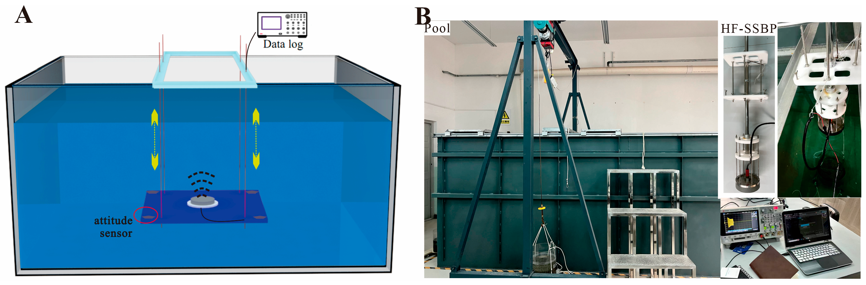
3.1. Experimental Equipment

In the experiment, a high-frequency submersible sub-bottom profiler (HF-SSBP) was developed by our team (Figure 1B). The HF-SSBP was specifically designed for precise and high-resolution measurement of an underwater substrate, and it has exceptional beam-focusing directivity and distance detection precision.

With a carrier frequency of 110 kHz and an operating bandwidth of 30 kHz, the HF-SSBP utilises the linear frequency-modulated (LFM) signal as a broadband signal and receives the echo as a coherent signal. In order to minimise the interference of the side lobe to the main lobe echo when the acoustic wave is emitted into the sediment, the transmitting and receiving signal functions of HF-SSBP are integrated into a single sensor to ensure that the side lobe main lobe ratio is 17.1 dB and the 3 dB beam width is 5.8 °. This design of the combined transducer maintains phase directionality for transmitting and receiving functions, effectively suppressing side lobe interference and minimizing transducer size. Cao (2021) used the HF-SSBP to measure deep-sea surface sediments and successfully obtained a fine sediment profile of 37 mm, from which the first sediment layer was extracted [36]. This practical validation demonstrates the feasibility of the HF-SSBP for fine-scale stratigraphic data measurements.

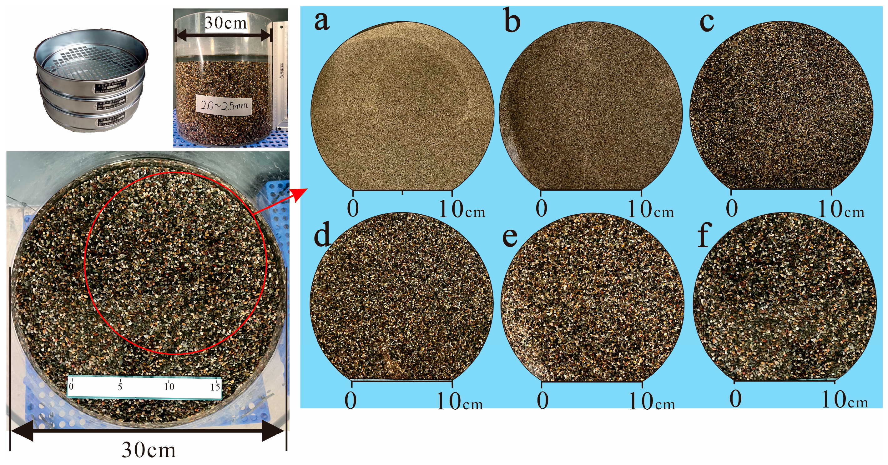
3.2. Sediment Preparation

The sediments used in this study were collected from the Kumarak River Basin, Aksu, Xinjiang. Through a comprehensive investigation of the acoustic reflectance properties of the sediments with various grain sizes in this basin, our objective was to enhance the classification of the silt sediments in the Xiaoshixia Reservoir area. The results provide precise and reliable substrate data support for the reservoir dredging project.

The sieve analysis method according to the Chinese national standard GB/T6003.1-2012 was used for the experiments. Before sieving, the sediment samples were dried and pre-treated, and the pre-treated sediments were then passed through six standardised sieves with mesh sizes of 0.1–0.3, 0.3–0.5, 0.5–1.0, 1.0–1.5, 1.5–2.0, and 2.0–2.5 mm, resulting in six homogeneous particle size sediments (Figure 2), which were then placed on the bottom of the pool to settle for 7 days. The primary focus of this paper is on the acoustic reflection characteristics of the sediment surface layer. In particular, the acoustic reflection characteristics between water and the sediment surface layer are of interest. When preparing the samples, a number of factors were considered, including sample preparation time, the settling process and the acoustic wavelength, in order to ensure the accuracy of the experimental results. Following meticulous preparation, the thickness of all samples was maintained at approximately 80 mm, enabling a more precise investigation of the acoustic reflection characteristics of the sediment surface layer and reducing the impact of extraneous variables on experimental outcomes.

To eliminate the impacts of air bubbles and fine particles that may be attached between the grains during the acoustic reflection test, we cleaned the deposits repeatedly. Then, we placed the cleaned deposits in a 3-millimetre-thick acrylic drum and used stirring and sedimentation methods to remove any remaining air bubbles from the deposits in the drum (Figure 2). To ensure the accuracy and consistency of our experimental data and to mitigate the impact of the different settling rates of the sediments with different grain sizes, we submerged them in a body of water and allowed them to settle and rest for a period of 10 days. We performed acoustic reflection tests on six sediments with uniform grain sizes and analysed the high-frequency reflection intensities of the sediments with different grain sizes at frequencies of 95–125 kHz. This method results in a more precise and dependable experimental outcome.

3.3. Tank Experiments

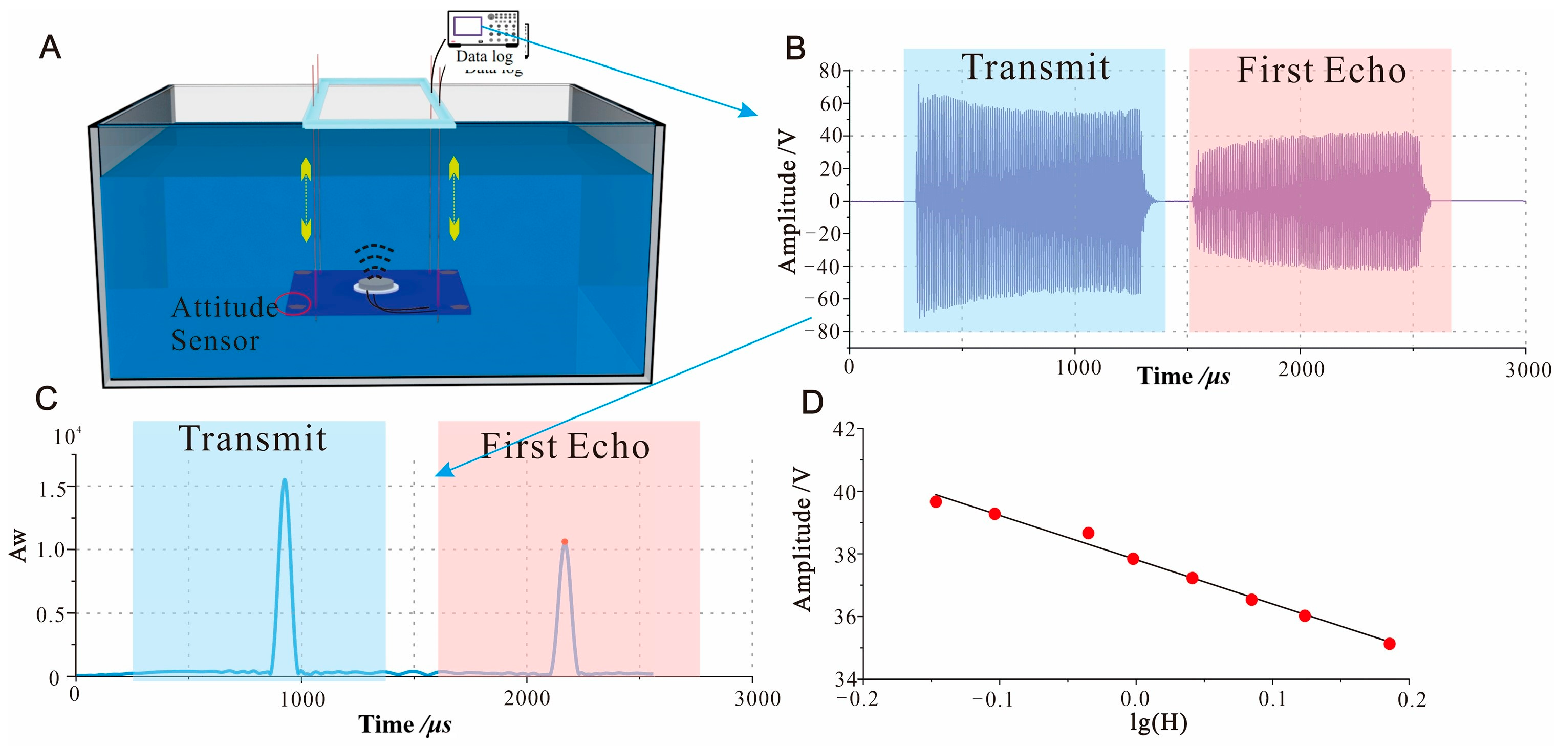
3.3.1. Acrylic Standard Plate Tank Experiment

To assess the feasibility of the experimental method, first, we carried out experimental tests on homogeneous acrylic sample panels. Based on the fact that the −3 dB beam angle of the combined transceiver sensor of the HF-SSBP is about 5.8°, the beam coverage diameter of the acoustic wave at 1 m of the propagation path is about 101 mm. To adequately cover the beam energy emitted by the transducer, we utilised a standard acrylic sample block (300 mm × 300 mm × 100 mm, L × W × H) during our experimental tests.

We positioned a typical acrylic sample block with a thickness of 100 mm at the bottom of a tank with a length of 4 m, a width of 2.5 m, and a depth of 1.7 m to examine its acoustic properties. To ensure precise measurements, we made certain that the transducer was placed directly above the sample block. We also ensured that the scattering angle of the transducer remained at 90° to the surface of the acrylic sample block (Figure 3A). The equipment frame was moved through plane motion, with the use of ray positioning to ensure that the equipment transducer and the centre of the acrylic plate were aligned. The length of the main rod connected to the transducer equipment was then adjusted, and ranging equipment was employed to ensure that the distance between the transducer surface and the surface of the sediment control was maintained, in order to measure the amplitude of the reflection at different ranges. The reflection coefficient of the acrylic sample block can be computed utilizing the measured reflection amplitude of the water-firm acrylic surface and the complete reflection amplitude of the calm water surface.

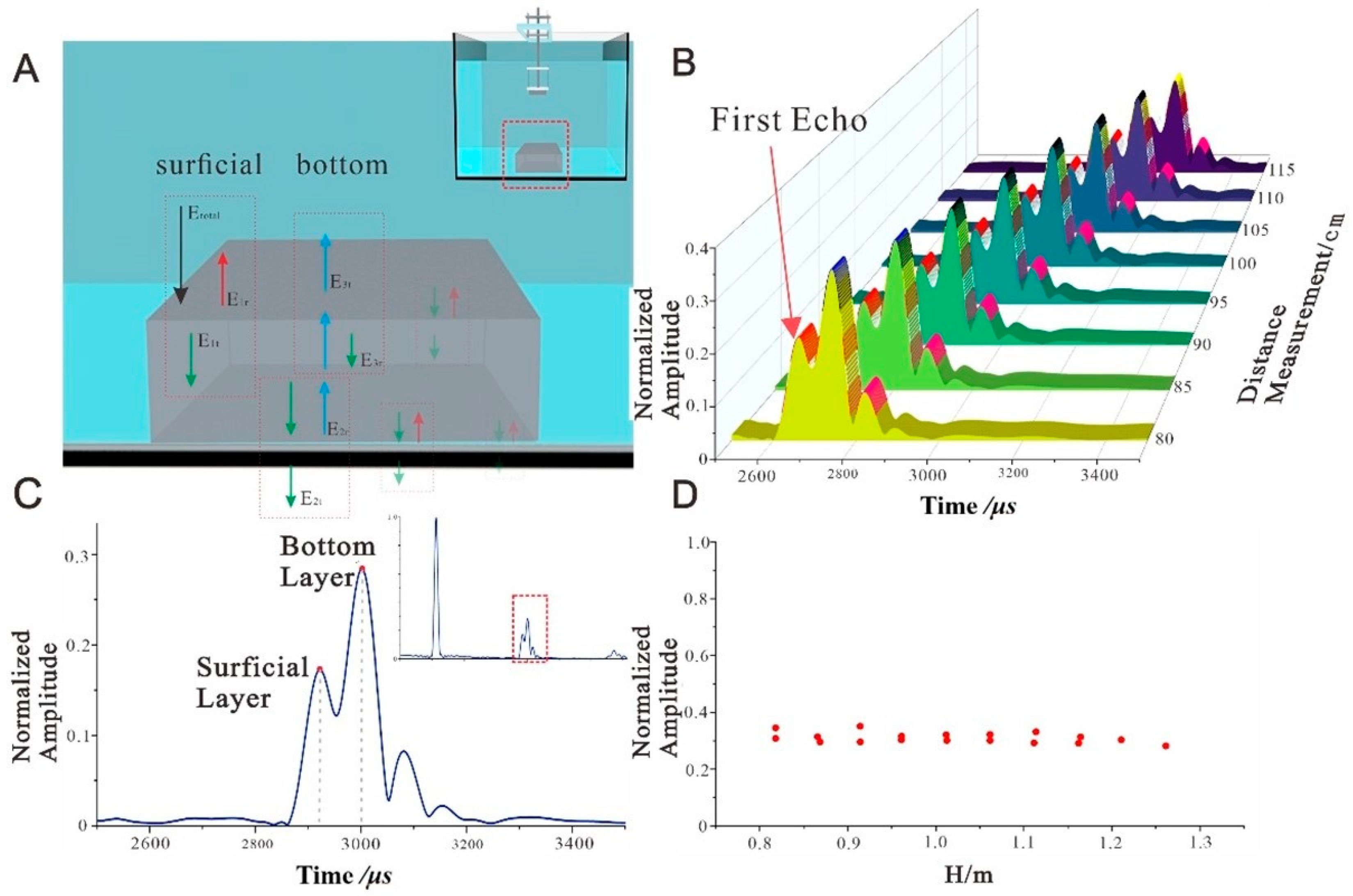
3.3.2. Sediment Tank Experiment

After conducting stability tests on a standard acrylic sample block, we measured six sediments with homogenous grain sizes within the frequency range of 95–125 kHz. We focused on the amplitude of the reflections from the water–sediment surface layer. Figure 3B displays the arrangement of the sediments with a consistent grain size within a 3-millimetre-thick acrylic drum situated within a swimming tank and incorporating a 100-millimetre-thick acrylic sheet as an undersurface. Uniformly sized sediments were placed in acrylic buckets with a thickness of 3 mm. These buckets were then positioned on a 100-millimetre-thick acrylic sheet, which served as the base of the tank. Before testing, we precisely measured the thickness of the deposit using a millimetre ruler. The device’s platform was precisely positioned on a flat surface using a ray positioning system to ensure that the transducer’s axis was aligned with the acrylic drum’s axis. Concurrently, the attitude sensor was meticulously calibrated to guarantee that the HF-SSBP device’s transducer remains level with the sediment surface, thus ensuring the precision and stability of the experiment or operation. During the experiments, sediments with different uniform grain sizes were utilised, and in the experiment, different uniform grain sizes of sediment were replaced, and the distance between the transducer and the sediment surface was controlled by adjusting the length of the main rod of the transducer device. The reflectance amplitude of the sediment was measured using this technique for different grain sizes and measuring distances from the water–sediment surface. The reflectance coefficients were then calculated.

4. Results and Discussion

4.1. Static Water Surface Total Reflection Test Results

Based on the experimental requirements and the tank height, we obtained the total reflection data from the HF-SSBP transducer device at the water surface within the range of 0.7–1.5 m. Figure 4B displays a time–domain plot of the static water surface total reflection at a distance of 1.0 m from the transducer device’s water surface. The outcome of the data pulse compression indicates that the initial peak corresponds to the amplitude of the transducer’s emission peak. The normalised reflection peak of the static water surface total reflection is represented by the red dot on the second peak in Figure 4C. By analysing the tested amplitude of static reflection from the water surface at different depths, a clear linear relationship between the device’s distance from the water surface and the total reflection amplitude of the static water surface was obtained (Figure 4D):

$$\log A_w=-17.655\lg \left(H\right)+37.853$$

(9)

where H is the distance from the transducer to the horizontal plane, and lg(Aw) is the magnitude of the water surface reflection amplitude measured by the transducer at a distance H from the still water surface. The reflectance amplitudes As and Aw can be derived by measuring the sediment reflectance amplitudes and total reflectance amplitudes at the still water surface within a laboratory setting, respectively. The reflection coefficients can be determined for distinct sediments by utilising the reflection coefficient formula.

4.2. Acrylic Sample Plate Sound Reflection Test Results

Figure 5A presents a schematic diagram of the interface acoustic wave propagation model in a water–acrylic medium using an acrylic sample block. Whenever the acoustic wave encounters a two-phase interface, it is transformed into a transmitted wave and a reflected wave. The reflection data of the reflected wave are then obtained using the HF-SSBP equipment.

Error measurements and stability tests were conducted on 100-mm-thick acrylic sample blocks. The measured thickness of the acrylic sample block was calculated using the time difference between the peak reflection time at the interface of the water–acrylic sample block (E1t) and the peak reflection time at the bottom of the acrylic sample block (i.e., the bottom of the pool (E2t)), obtained via compression processing of the pulse data (Figure 5B). By measuring the measured thickness and the true thickness error, the absolute error and stability of the HF-SSBP in the high-frequency reflection intensity measurement were effectively verified.

Statistical analysis of the two peak intervals was conducted through pulse compression processing for different ranges (Figure 5C). The analysis revealed that the time intervals were 79–80 μs, demonstrating consistency. The thicknesses of the acrylic were calculated to be 106.334 and 107.68 mm using the standard speed of sound for acrylic (2692 m/s) (data indexed using the procedure of Hamilton (1972)) and the time intervals. The measurements had an absolute error of 7.7 mm. The measurement results are consistent with those of Cao et al. (2022), which verifies the accuracy and reliability of the HF-SSBP equipment in measuring acrylic sample plates at different ranges. These results provide strong support for further research on sediment acoustic reflection properties.

We analysed the reflection characteristics of E1r, which is the reflected first echo, based on 100-millimetre-thick acrylic sample blocks at different ranges (Figure 5C). The surface reflection data for the acrylic sample block were measured at different measurement distances by adjusting the distance between the transducer and the surface of the block. Our analysis of the pulse compression over various measurement distances revealed that the amplitude of the reflection on the surface of the water–acrylic sample block decreased with increasing distance. Our analysis of the pulse compression over various measurement distances revealed that the amplitude of reflection on the surface of the water–acrylic sample block decreased with increasing distance. Equation (7) was utilised to determine the total reflection amplitude Aw for each range corresponding to the still water surface. This was then utilised to calculate the reflection coefficients of the 100-mm-thick acrylic sample block at various measurement distances (Figure 5D). The reflection coefficient of the acrylic sample block was measured within the range of 0.8–1.15 m, and it was found to have an average value of 0.318. In addition, the reflection coefficient of the acrylic sample block extracted from the transducer with a spacing of 1 m was measured to be 0.320. These results are consistent with the findings of Cao et al. (2022) in their calibration experiments using an HF-SSBP. These findings provide a foundation for the reliability of subsequent experiments measuring the reflection coefficient of sediments.

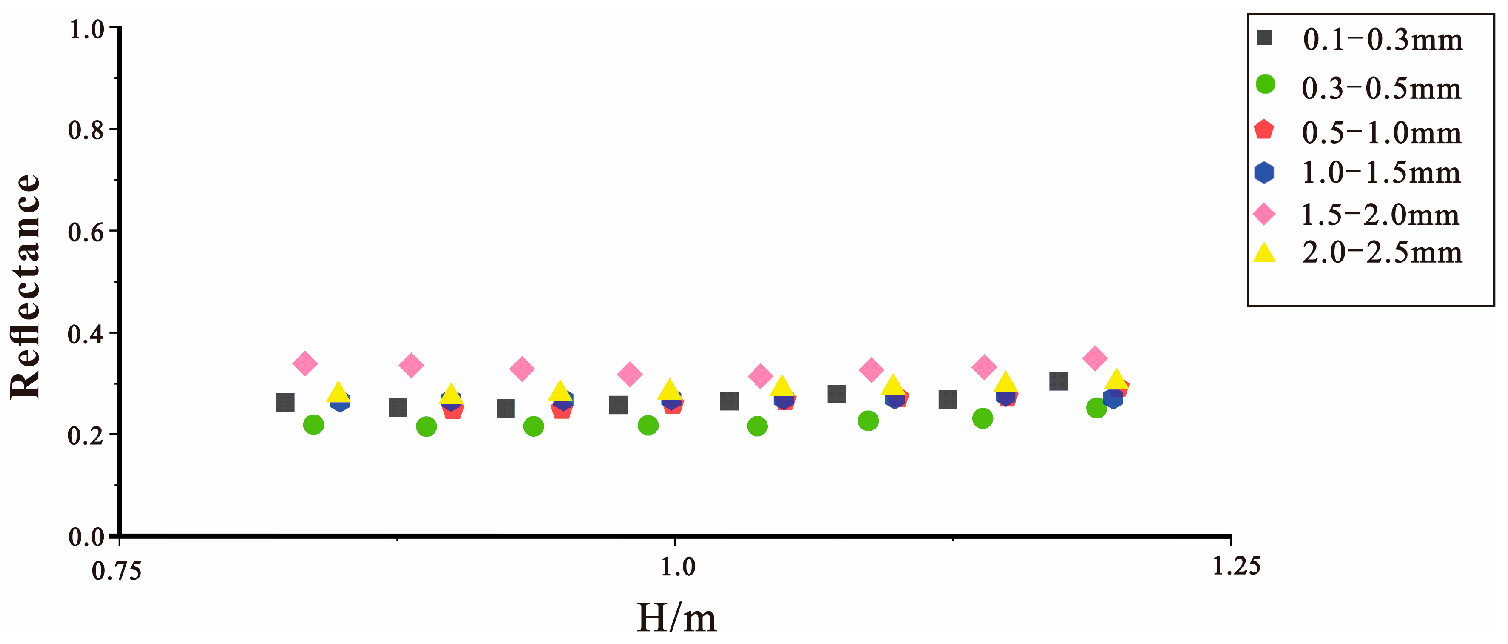
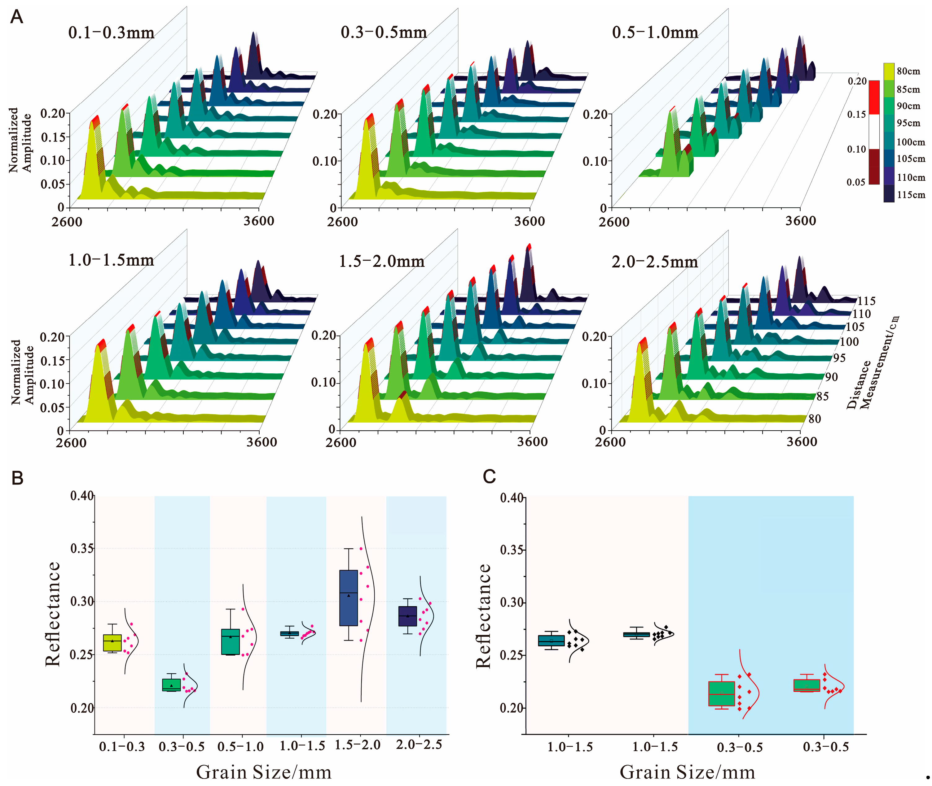
4.3. Sediment Reflection Coefficient Measurements

Mechanical adjustment of the device to the surface of the sediment was conducted to measure the distance. The reflection amplitudes of the sediment were measured for different homogeneous grain sizes and measurement distances. The formula for the reflection coefficient was utilised to compute the reflection coefficients for the water–sediment surface at diverse homogeneous grain sizes, in combination with the laboratory total reflection test data for a static water surface.

In order to ensure the accuracy of the experimental equipment, we conducted a comprehensive data extraction and analysis. By applying pulse compression to the data (Figure 5C), we statistically analysed the peak-to-peak intervals of reflections between the water–sediment surface layer and the sediment bottom-acrylic interface at varying measuring distances (

Table 2. Time difference between water–sediment surface and sediment–acrylic acoustic reflection (μs).

	Distance Measurement	Time Difference Between Water–Sediment Surface and Sediment–Acrylic Acoustic Reflection (μs)
		80 cm	85 cm	90 cm	95 cm	100 cm	105 cm	110 cm	115 cm
Grain size	0.1–0.3 mm	83	84	85	84	85	85	85	85
	0.3–0.5 mm	69	69	69	70	70	70	69	70
	0.5–1.0 mm	81	81	81	80	80	80	80	-
	1.0–1.5 mm	83	84	84	84	84	83	83	83
	1.5–2.0 mm	73	74	75	75	76	76	77	77
	2.0–2.5 mm	73	73	73	72	72	72	73	73

). In our experiments, we maintained a constant sediment thickness at a specific grain size. Theoretically, the measured time difference between the two peaks should be consistent when changing the measuring distance. However, if the time difference data appear inconsistent, it indicates that there are variables in the testing process that affect the testing accuracy.

Upon examination of the data, it was observed that the time intervals between the peaks of the reflection peaks at the water–sediment surface layer and the bottom of the sediment–acrylic interface were essentially the same for all conditions, with the exception of the 1.5–2.0 mm grain size sediments tested. The test time intervals exhibited a discrepancy of approximately 2 μs when the thickness was held constant. For sediments with a grain size of 1.5–2.0 mm, we hypothesise that this discrepancy is primarily attributable to the sediments being subjected to impact during testing, resulting in re-settlement, which subsequently affects the time interval of the reflection peaks. Further research is to be conducted on the subject of sediment settling times in relation to reflection coefficients.

By analysing the test results for the sediments with different grain sizes within the same measurement range, it was found that the surface reflection coefficients of the six grain sizes (Figure 6) exhibited a relatively stable fluctuation. However, the reflection coefficients of the sediment with a grain size of 1.5–2.0 mm were significantly larger than those of the other five grain sizes at the same measurement range due to external fluctuations. The reflection coefficients of the sediment with a grain size of 2.0–2.5 mm were relatively larger (Figure 6), while the sediment with a grain size of 0.3–0.5 mm had the smallest reflection coefficients. There was no significant variability in the reflection coefficients of the sediments with grain sizes of 1.0–1.5, 0.5–1.0, and 0.1–0.3 mm at the same distance.

Figure 7A illustrates the changes in the water–sediment surface reflectance amplitude at different ranges for the same grain size. Figure 7A shows that there is a significant negative correlation between the reflection amplitude of the sediment particles with six grain sizes and the test distance from the equipment to the sediment surface. Statistical analyses were conducted on the reflectance coefficients of the six sediments (Figure 7B). For the sediment with a grain size of 0.3–0.5 mm, the water–sediment surface layer’s average reflection coefficient was 0.225 at varying measuring distances, with a standard deviation of 0.012. In addition, the average scattering intensity of the 0.3–0.5 mm sediment was –12.97 dB. The mean reflection coefficient of the water–sediment surface layer at different ranges of 0.5–1.0 mm was 0.267, with a standard deviation of 0.014. The mean scattered intensity was −11.48 dB. The average water–sediment surface reflection coefficient had a mean value of 0.270 and a standard deviation of 0.003 over different ranges of 1.0–1.5 mm, while the average scattering intensity was recorded as −11.35 dB. The average reflectance coefficient of the 2.0–2.5 mm water–sediment surface layer was 0.286, with a standard deviation of 0.010, and the average scattering intensity was −10.86 dB. The aforementioned four sediments exhibited a positive correlation between the reflection coefficients of the water–sediment surface layer and the grain size of the sediment.

For the sediments with a grain size of 0.1–0.3 mm, the mean reflection coefficient of the water–sediment surface layer at various measuring distances was 0.268, with a standard deviation of 0.012, and the mean scattered intensity value was −11.44 dB. By contrast, the mean scattered intensity of the water–sediment surface layer for the granular material with a size of 1.5–2.0 mm at varying measurement distances was −10.30 dB, and the mean reflection coefficient was 0.305, with a standard deviation of 0.028. The mean reflection coefficient was 0.305, with a standard deviation of 0.028. The reflectance intensity dispersion coefficients for the five sediments with different grain sizes at different ranges were all less than 5%, except for the 1.5–2.0 mm sediments, which had a relatively large standard deviation for the reflectance coefficients. This may be due to the sediment fluctuations caused by the sediment movement process and requires further confirmation in future studies.

To ensure the accuracy and reliability of the experimental testing process, sediment samples with grain sizes of 0.3–0.5 to 1.0–1.5 mm were prepared simultaneously. Subsequent testing of these parallel samples revealed the following findings (Figure 7C): for sediments with a grain size of 0.3–0.5 mm, the average reflection coefficients were 0.225 and 0.220, and the average intensities of the surface scattering were −12.97 and −13.15 dB, respectively. For the 1.0–1.5 mm sediments, the average reflection coefficients were 0.270 and 0.264, and the average surface scattering intensities were −11.35 and −11.57 dB, respectively. The experimental data exhibit some stability, as evidenced by the relatively small difference between the reflection coefficient and the scattering intensity of the two groups of parallel samples.

5. Conclusions

There are notable contrasts in the acoustic reflectance properties of different environments and sediment types. To accurately and efficiently obtain data on the acoustic reflectance properties of sediments with different grain sizes. Indoor acoustic reflectance measurements were conducted on six sediment samples with different grain sizes in a specific environment using an HF-SSBP. The results of the study are as follows:

(1) We measured the amplitude of the total reflected echoes on a still water surface at varying propagation distances. We found that there is a strong linear relationship between the intensity of the reflected echo and the logarithm of the water depth.

(2) The time difference between the first and second reflected waves of a 100-mm-thick acrylic sample block was extracted at different ranges. The thickness of the acrylic sample block was measured by calculating the time difference. The absolute value of the measurement error was within 7.7 mm at various ranges compared with the actual thickness, indicating the error’s stability at different HF-SSBP ranges.

(3) The reflection coefficients of the 100-mm-thick acrylic samples remained stable across different measurement ranges. This fragment reflects the test’s reliability and the stability of the HF-SSBP at different measurement distances.

(4) The scattering intensity of the six sediments with uniform grain size distributions at the same measurement distance varied to some extent. There was variation in the intensity of the acoustic wave reflections for the different grain sizes, but some of the differences were not statistically significant.

(5) The dispersion coefficients of the acoustic reflection intensities for all of the sediments, except for those with a grain size of 1.0–1.5 mm, were less than 5% at different measurement distances. These coefficients were almost independent of the detection distance.

An accurate measurement study was conducted utilising the HF-SSBP on six sediments with grain sizes ranging from 0.1 to 2.5 mm in a specific environment. The experimental results demonstrate that these sediments with different grain sizes exhibit significant variability in acoustic reflection intensity. Further analysis indicates that the dispersion of the acoustic reflection intensity coefficients of these sediments is low and stable within the range of 5% at different measurement distances. This proves that the HF-SSBP method has high accuracy and stability in measuring the acoustic reflection coefficients of the substrate sediments.

This study has the following limitations that need to be addressed: First, the experimental samples only encompass six types of homogeneous sediments with grain sizes ranging from 0.1 to 2.5 mm, leaving the acoustic characteristics of finer-grained particles and heterogeneous mixed sediments unexplored. Second, technical constraints exist in the detection resolution of low-frequency signals by the experimental setup, and the dynamic factors of real marine environments were not fully simulated. Future research should prioritise systematic testing of submillimeter-scale fine-grained sediments and multi-grain-size mixed sediments. Concurrently, improvements in the spatiotemporal resolution of data acquisition should be achieved through optimised sensor array configurations or in-situ monitoring experiments. These enhancements will facilitate the establishment of a more comprehensive sediment acoustic characteristics database, providing high-confidence foundational datasets for application fields such as marine geological exploration and subsea resource assessment.

References

1. Liu, B.H.; Kan, G.M.; Li, G.B.; Yu, S.Q. Measurement Techniques and Applications of Acoustic Properties of Submarine Sediments; Science Press: Beijing, China, 2019. [Google Scholar]
2. Oelze, M.L.; Sabatier, J.M.; Raspet, R. Roughness measurements of soil surfaces by acoustic backscatter. Soil Sci. Soc. Am. J. 2003, 67, 241–250. [Google Scholar] [CrossRef]
3. Stanic, S.; Briggs, K.B.; Fleischer, P.; Sawyer, W.B.; Ray, R.I. High-frequency acoustic backscattering from a coarse shell ocean bottom. J. Acoust. Soc. Am. 1989, 85, 125–136. [Google Scholar] [CrossRef]
4. Gallaudet, T.C.; de Moustier, C.P. High-frequency volume boundary acoustic backscatter fluctuations in shallow water. J. Acoust. Soc. Am. 2003, 114, 707–725. [Google Scholar] [CrossRef]
5. Boyle, F.A.; Chotiros, N.P. A model for acoustic backscatter from muddy sediments. J. Acoust. Soc. Am. 1995, 98, 525–530. [Google Scholar] [CrossRef]
6. Liu, B.H.; Han, T.C.; Kan, G.M.; Li, G.B. Correlations between the in situ acoustic properties and geotechnical parameters of sediments in the Yellow Sea, China. J. Aslan Earth Sci. 2013, 77, 83–90. [Google Scholar] [CrossRef]
7. Huang, Z.; Siwabessy, J.; Cheng, H.; Nichol, S. Using multibeam backscatter data to investigate sediment-acoustic relationships. J. Geophys. Res-Ocean. 2018, 123, 4649–4665. [Google Scholar] [CrossRef]
8. Wang, J.Q.; Li, G.B.; Kan, G.M.; Liu, B.H.; Meng, X.M. Experiment study of the in-situ acoustic measurement in seafloor sediments from deep sea. Chin. J. Geophys. 2020, 63, 4463–4472. Available online: http://www.geophy.cn/article/doi/10.6038/cjg2020N0427 (accessed on 27 March 2025).
9. Rizvi, Z.H.; Mustafa, S.H.; Sattari, A.S.; Ahmad, S.; Furtner, P.; Wuttke, F. Dynamic lattice element modelling of cemented geomaterials. In Advances in Computer Methods and Geomechanics: IACMAG Symposium; Springer: Singapore, 2019; Volume 1, pp. 655–665. [Google Scholar]
10. Trzcinska, K.; Tegowski, J.; Pocwiardowski, P.; Janowski, L.; Zdroik, J.; Kruss, A.; Rucinska, M.; Lubniewski, Z.; Schneider von Deimling, J. Measurement of seafloor acoustic backscatter angular dependence at 150 kHz using a multibeam echosounder. Remote Sens. 2021, 13, 4771. [Google Scholar] [CrossRef]
11. Williams, K.L.; Jackson, D.R.; Tang, D.; Briggs, K.B.; Thorsos, E.I. Acoustic backscattering from a sand and a sand/mud environment: Experiments and data/model comparisons. IEEE J. Ocean. Eng. 2009, 34, 388–398. [Google Scholar] [CrossRef]
12. Vicki, F.L.; Roger, F.D. The effects of fine-scale surface roughness and grain size on 300 kHz multibeam backscatter intensity in sandy marine sedimentary environments. Mar. Geol. 2006, 228, 153–172. [Google Scholar] [CrossRef]
13. Yu, S.Q.; Liu, B.H.; Yu, K.B.; Yang, Z.G.; Kan, G.M.; Zhang, X.B. Comparison of acoustic backscattering from a sand and a mud bottom in the South Yellow Sea of China. Ocean Eng. 2020, 202, 107145. [Google Scholar] [CrossRef]
14. Zou, D.P.; Ye, G.C.; Liu, W.; Sun, H.; Li, J.; Xiao, T.B. Effect of temperature on the acoustic reflection characteristics of seafloor surface sediments. J. Ocean Univ. China 2022, 21, 62–68. [Google Scholar] [CrossRef]
15. Zou, D.P.; Xie, J.; Meng, X.M.; Han, S.; Feng, J.C.; Kan, G.M. Analysis of the variation of in situ seafloor sediments acoustic characteristics with porosity based EDFM. Front. Mar. Sci. 2023, 10, 1270673. [Google Scholar] [CrossRef]
16. McKinney, C.M.; Anderson, C.D. Measurements of Backscatterin of Sound from the Ocean Bottom. J. Acoust. Soc. Am. 1964, 36, 158–163. [Google Scholar] [CrossRef]
17. Jackson, D.R.; Baird, A.M.; Crisp, J.J.; Thomson, P.A.G. High-frequency bottom backscatter measurements in shallow water. J. Acoust. Soc. Am. 1986, 80, 1188–1199. [Google Scholar] [CrossRef]
18. Yu, S.Q.; Liu, B.H.; Yu, K.B.; Yang, Z.G.; Kan, G.M. Backscattering Characteristics over a Wide Band of a Sand Bottom in the South Yellow Sea of China. In Proceedings of the 2021 OES China Ocean Acoustics (COA), Harbin, China, 14–17 July 2021; pp. 86–90. [Google Scholar]
19. Weber, T.C.; Ward, L.G. Observations of backscatter from sand and gravel seafloors between 170 and 250 kHz. J. Acoust. Soc. Am. 2015, 138, 2169–2180. [Google Scholar]
20. Hines, P.C.; Osler, J.C.; MacDougald, D.J. Acoustic backscatter measurements from littoral seabeds at shallow grazing angles at 4 and 8 kHz. J. Acoust. Soc. Am. 2005, 117, 3504–3516. [Google Scholar] [CrossRef]
21. Radhakrishnan, S.; Anu, A.P. Characterization of seafloor roughness from high-frequency acoustic backscattering measurements in shallow water off the west coast of India. J. Acoust. Soc. Am. 2020, 148, 2987–2996. [Google Scholar] [CrossRef]
22. Tian, Y.H.; Wu, L.; Zou, D.P.; Chen, Z.; Jiang, Y.J.; Yan, P.; Fan, C.Y. Predicting the acoustic characteristics of seafloor sediments containing cold spring carbonate rocks. Front. Mar. Sci. 2023, 10, 1243780. [Google Scholar] [CrossRef]
23. Kan, G.M.; Liu, B.H.; Yang, Z.G.; Yu, S.Q.; Qi, L.H.; Yu, K.B.; Pei, Y.L. Acoustic backscattering measurement from sandy seafloor at 6–24 kHz in the South Yellow Sea. Acta Oceanol. Sin. 2019, 38, 99–108. [Google Scholar] [CrossRef]
24. Stanic, S.; Briggs, K.B.; Fleischer, P.; Ray, R.I.; Sawyer, W.B. Shallow-water high-frequency bottom scattering off Panama City, Florida. J. Acoust. Soc. Am. 1988, 83, 2134–2144. [Google Scholar] [CrossRef]
25. Liu, B.H.; Kan, G.M.; Pei, Y.L.; Yang, Z.G.; Yu, S.Q.; Yu, K.B. A review on the progress of bottom acoustic scattering research. Haiyang Xuebao 2017, 39, 1–11. (In Chinese) [Google Scholar]
26. He, L.B.; Zhao, J.H.; Lu, J.H.; Qiu, Z.G. High-accuracy acoustic sediment classification using sub-bottom profile data. Estuar. Coast. Shelf Sci. 2022, 265, 107701. [Google Scholar] [CrossRef]
27. Wendelboe, G.; Hefner, T.; Ivakin, A. Observed correlations between the sediment grain size and the high-frequency backscattering strength. JASA Express Lett. 2023, 3, 2. [Google Scholar] [CrossRef]
28. Curlander, J.C.; McDonough, R.N. Synthetic Aperture Radar: Systems and Signal Processing; Wiley: New York, NY, USA, 2021. [Google Scholar]
29. Kan, G.M.; Liu, B.H.; Zhao, Y.X.; Li, G.B.; Pei, Y.L. Self-contained in situ sediment acoustic measurement system based on hydraulic driving penetration. High Technol. Lett. 2011, 17, 311–316. [Google Scholar]
30. Thorne, P.D.; Hurther, D. An overview on the use of backscattered sound for measuring suspended particle size and concentration profiles in noncohesive inorganic sediment transport studies. Cont. Shelf Res. 2014, 73, 97–118. [Google Scholar] [CrossRef]
31. Smerdon, A.; Van Der, A.; To, M. Measurement of Near-Bed sediment load, particle size, settling velocity and turbulence from a multi-frequency acoustic backscatter instrument. In Coastal Sediments 2023: The Proceedings of the Coastal Sediments; World Scientific: Singapore, 2023; pp. 1597–1606. [Google Scholar]
32. Sternlicht, D.D.; de Moustier, C.P. Time-dependent seafloor acoustic backscatter (10–100 kHz). J. Acoust. Soc. Am. 2003, 114, 2709–2725. [Google Scholar] [CrossRef]
33. Wei, P.; Wang, C. Effects of grain size distributions on scattering attenuation of elastic waves in polycrystalline materials. Acta Mech. 2024, 235, 3231–3244. [Google Scholar] [CrossRef]
34. Qu, Z.G.; Cao, X.H.; Shen, B.J.; Zhang, Y.H. Near bottom acoustic detection of canyon Mousse layers in the South China Sea. Acta Acust. 2021, 46, 220–226. [Google Scholar] [CrossRef]
35. Cao, X.H.; Qu, Z.G.; Shen, B.J.; Zhang, H.Y. Illuminating centimeter-level resolution stratum via developed high-frequency sub-bottom profiler mounted on Deep-Sea Warrior deep-submergence vehicle. Mar. Georesour. Geotechnol. 2021, 39, 1296–1306. [Google Scholar] [CrossRef]
36. Cao, X.; Zou, D.; Qu, Z.; Zhen, H.; Cheng, H.; Wei, Z. Calibration and application of high-frequency submersible sub-bottom profiler for deep-sea surficial sediment measurement. Mar. Georesour. Geotechnol. 2022, 41, 671–681. [Google Scholar] [CrossRef]
Figure 1. Schematic diagram of the water surface total reflection test method (A) and experimental tank and high-frequency broadband narrow-beam single-transducer probe (B).
Jmse 13 00741 g001
Figure 2. Sediment sample preparation and images. Sediment grain size 0.1-0.3 (a); Sediment grain size 0.3-0.5 (b); Sediment grain size 0.5-1 (c); Sediment grain size 1.0–1.5 (d); Sediment grain size 1.2–2.0 (e); Sediment grain size 2.0–2.5 (f).
Jmse 13 00741 g002
Figure 3. Schematic diagrams of (A) the acrylic standard plate tank experiment and (B) the sediment test experiment (processed using 3 ds Max).
Jmse 13 00741 g003
Figure 4. Plot of static water surface total reflection test results. (A) Schematic diagram of measurement of the total reflection on a still water surface. (B,C) Total reflection and pulse compression results, respectively, at the still water surface with a range of 1 m. (D) Plot of the reflection amplitude at the still water surface against the logarithm of the range.
Jmse 13 00741 g004
Figure 5. Acrylic sample sound reflection test data graph. (A) Schematic diagram showing the acoustic reflection from an acrylic surface layer. (B) Plots of the reflection amplitudes at different ranges of the acrylic, and (C) the pulse compression results of the reflection amplitude at a range of 1 m. (D) Reflection coefficient plotted against the acrylic surface layer for various measurement ranges.
Jmse 13 00741 g005
Figure 6. Reflection coefficient versus ranging plots for six grain-size homogeneous sediments.
Jmse 13 00741 g006
Figure 7. (A) Reflectance amplitude at different ranges for six sediments, and (B) reflectance coefficient relationships. (C) Reflection coefficients for parallel samples of 1.0–1.5 mm and 0.3–0.5 mm sediments.
Jmse 13 00741 g007