Abstract
To enhance the autonomy of semi-submersibles, a Model Predictive Control (MPC) strategy was proposed based on real-time Line-of-Sight (LOS) to address the issue of thruster saturation. By identifying parameters using experimental data from sea trials, the dynamic model of the semi-submersible was derived and established. The kinematic and dynamic models were combined to construct a complete MPC prediction model, and the LOS method was integrated into the MPC strategy to achieve trajectory-tracking functionality. Unlike prior research that was validated exclusively through simulations, this paper further validated the efficacy of the improved LOS-MPC in real path tracking through a series of sea trials. The experimental findings indicate that the improved LOS-MPC approach is capable of rapidly guiding the semi-submersible to precisely follow the reference trajectory. In comparison to conventional PID controllers, the LOS-MPC-based path-tracking controller demonstrates enhanced effectiveness in terms of response speed, tracking accuracy, and robustness.
1. Introduction
As maritime activities such as search and rescue, military operations, seabed mapping, and resource exploration [1] become more prevalent, the associated scientific and technological fields continue to advance [2,3]. To accomplish these complex tasks, it is crucial to adopt practical and cost-effective methods, and the collaboration of multiple Autonomous Underwater Vehicles (AUVs) is key [4,5,6,7]. Compared with a single AUV, the collaboration of multiple AUVs offers significant advantages in flexibility, controllability, and safety.
A Semi-Submersible Offshore Platform (SSOP) is a special type of marine platform or underwater equipment, characterized by its partial submersion in water to enhance stability and adaptability. It is commonly used in marine missions such as scientific research, engineering, and resource development. The main body of the SSOP is designed to be partially immersed in water, which not only enhances its ability to withstand wind and waves but also reduces the possibility of detection, making up for the lack of concealment of traditional underwater equipment [8]. Therefore, the SSOPs are particularly suitable for tasks such as military reconnaissance, covert monitoring, and exploration of sensitive areas.
In recent years, significant research has been conducted on the path-tracking control of underwater robots [9]. Sliding mode control (SMC) is extensively utilized in subaquatic trajectory monitoring due to its strong resilience to model uncertainties [10,11,12]. In the literature [13], sliding mode control is integrated with the PID method to improve path-tracking performance. A major challenge in sliding mode control is the “chattering” effect, which limits its practical application. To mitigate this issue, the literature [14] proposed a novel adaptive term to design a chatter-free sliding mode controller. Beyond sliding mode approaches, neural network algorithms have also been widely adopted for underwater path tracking. An efficient single-layer neural network method is proposed for path tracking in the literature [15]. In the literature [16], Dynamic Surface Control is combined with Minimal Learning Parameters to design a novel adaptive neural network tracking controller, utilizing RBF neural networks to interpret tracking errors. Simulation results showed that the algorithm effectively reduces the tracking error to a small vicinity around the target path. Neural network-driven motion regulation remains unaffected by the robot’s dynamic model while demonstrating excellent adaptability [17]. However, the complex underwater environment increases the difficulty of the training and learning processes, thereby reducing the real-time efficiency. Backstepping control is also extensively utilized for path-tracking tasks of underwater robots. The literature [18] introduced an algorithm that integrates a biologically motivated model-driven filter incorporated alongside backstepping control to facilitate three-dimensional trajectory following of crewed submersibles. Experimental findings demonstrated that the proposed method attained effective trajectory regulation. However, the frequent challenge with backstepping control is that when tracking errors are significant, the speed is abruptly elevated, leading to a decline in tracking performance.
Although the aforementioned path-tracking control studies have achieved good results, practical system constraints, such as actuator saturation, must still be considered in real applications. To overcome these practical limitations in controller design, Model Predictive Control (MPC) is considered an ideal algorithm. MPC effectively handles hard constraints through the optimization process and has become a hot topic in path-tracking research for underwater robots in recent years [19]. In the literature [20], researchers integrated path planning and path-tracking problems and solved them utilizing nonlinear MPC. To enhance the efficiency of addressing the optimization challenge, the literature [21] introduced a logarithmic barrier function as part of the objective function and improved the C/GMRES algorithm to fit the traditional MPC method. The literature [22] proposed a new scheme based on nonlinear model predictive control (NMPC) for trajectory tracking management, with the advantage of ensuring closed-loop stability of optimization-based path-tracking control. However, the high computational cost of NMPC affects its practicality. To address this, the literature [23] developed a distributed NMPC algorithm to reduce computational costs while maintaining closed-loop steadiness. Despite the progress made in the aforementioned path-tracking control algorithms, most studies are primarily based on underwater vehicle models and validated through numerical simulations. The literature [24] proposed a real-time nonlinear Model Predictive Control strategy that transforms the obstacle avoidance problem into a variable constraint problem for solution. The literature [25] experimentally validated the depth control of an AUV using Linear Time-Varying MPC (LTV-MPC), but it did not involve path-tracking experiments. The literature [24] proposed a real-time NMPC scheme that reformulates obstacle avoidance as a variable constraint problem. The literature [25] validated depth control using LTV-MPC but did not involve path-tracking experiments. In addition, the literature [26] proposed an adaptive sliding mode control approach to enhance the dynamic positioning performance of an SSOP. This method significantly improved position-keeping accuracy and disturbance rejection capability in complex marine environments. However, its limitations include high computational complexity, significant hardware burden, difficulty in parameter tuning, and the need for further research and validation of long-term reliability and wide applicability.
This paper investigates the path-tracking problem of the SSOP under thrust constraints. Guided by [22], this study designs a path-tracking controller based on a Model Predictive Control (MPC) algorithm. The main contributions are threefold: First, kinematic and dynamic models of the SSOP are established through consideration of the longitudinal and yaw degrees of freedom to construct the predictive model of the SSOP. Second, a Line-of-Sight (LOS)-based MPC control algorithm is designed to address the poor path-tracking performance of the SSOP. Third, the proposed algorithm is evaluated through simulations and experiments.
The organization is as follows: Section 2 outlines the design of the SSOP; Section 3 elaborates on system modeling and identification; Section 4 describes the LOS-MPC-based path-tracking controller; and Section 5 presents the experimental results and compares and analyzes other path-tracking algorithms. Finally, Section 6 provides a summary of the research findings and discusses future research directions.
2. Design of the SSOP
2.1. The Concept of the SSOP
The SSOP is a fully Autonomous Underwater Vehicle capable of navigating underwater autonomously and performing exploration and monitoring tasks. Its main functions include multi-degree-of-freedom motion in space, long-endurance navigation, autonomous route planning, high-precision real-time navigation and positioning, mission detection operations, data storage, and real-time data transmission.
The vehicle’s main structure integrates carbon fiber-reinforced composite materials and syntactic foam, forming an integrated composite structure. Rib plates are used to enhance the overall strength and rigidity of the hull, while high-strength buoyancy materials are bonded and encapsulated within the carbon fiber shell to form a unified structure, thereby further increasing its strength and rigidity. Based on this structural foundation, the energy system, propulsion system, control system, navigation and positioning system, communication system, and mission payload units are deployed. The comprehensive structural arrangement of the SSOP is depicted in Figure 1, and its overarching framework is illustrated in Figure 2.
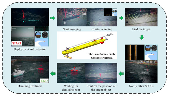
Figure 1.
Schematic diagram of the SSOP in a seabed zone.
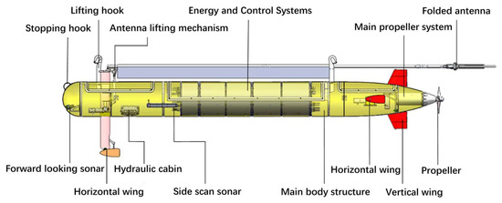
Figure 2.
The structure of the semi-submersible platform.
2.2. The Control System
The system of the SSOP described in this paper is shown in Figure 3. It is centered around a central processing unit and divided into three subsystems: the main control subsystem, the propulsion drive subsystem, and the payload control subsystem. The main control subsystem consists of the core main control unit, sensor unit, and communication and processing unit. These three units are integrated onto a single circuit board, which not only decomposes functions to reduce the processing load on the central processor but also achieves high integration, reducing the cabling between hardware components and thereby enhancing overall system stability.
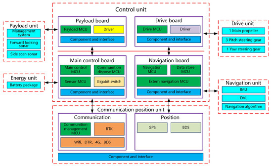
Figure 3.
The control system framework of the semi-submersible platform.
The energy unit is composed of a 22 kWh/48 V lithium battery pack and a Battery Management System (BMS), which supplies power to all electrical equipment of the SSOP. The propulsion unit employs a single propeller at the stern for propulsion, with heading changes achieved by controlling the vertical rudder and roll and pitch operations realized by adjusting the fore and aft horizontal control surfaces, thereby improving propulsion efficiency and control accuracy. The navigation unit incorporates an Inertial Measurement Unit (IMU), a Doppler Velocity Log (DVL), and navigation algorithms. The navigation unit transmits the combined results in real time to the main control system of the vehicle, which uses this data as the input position information to achieve position control during the vehicle’s operation. The communication and positioning unit includes modules such as the BeiDou Navigation Satellite System (BDS), data radio, RTK antenna, 4G, and WiFi. The various surface communication system modules are integrated into an antenna box of a folding antenna and connected to the control compartment via two cables. They can receive data sent from the main control system, process the data further, and then broadcast the data to the ground units of each communication device. The payload unit is composed of a payload management system, a PC, and a router, with external payload devices able to exchange, store, and process data with the PC.
The following sections will focus on the research of the control unit as well as the navigation and positioning unit.
3. System Modeling and Identification
3.1. Kinematic Modeling
For the SSOP AUV, the kinematics of the robot is defined relative to two coordinates, namely the inertial coordinate system (OI-XIYIZI) and the body coordinate system (OB-XBYBZB) [27]. The inertial coordinate system is a fixed Earth-referenced frame, typically defined using the North–East–Down (NED) convention, while the body coordinate system moves with the vehicle and is attached to its center of mass or buoyancy. The vehicle’s motion is described in six degrees of freedom (6 DOF), consisting of translational motion (position and velocity) and rotational motion (roll, pitch, and yaw), which define its orientation relative to the inertial frame. The transformation between these coordinate systems is handled through rotation matrices or quaternions, accounting for environmental disturbances such as currents and waves.
In this paper, due to the low center of gravity of the SSOP, it has a large restoring moment in its design, allowing it to quickly return to equilibrium under external disturbances and reducing roll angle variations. In addition, the semi-submersible structure enhances its stability, and the submerged portion provides damping, reducing the impact of waves on roll motion. Therefore, roll motion can be neglected. The three-degree-of-freedom kinematics of the SSOP is established in the right-hand coordinate system, as shown in Figure 4. Because only the motion on the water surface is considered, the position and direction of the robot are defined as relative to the center of mass, the submersible’s forward direction is determined in relation to the XI axis, and the clockwise direction is positive. The location and orientation of the SSOP are defined as follows: . The longitudinal, lateral, and turning angular velocities in the body coordinate system are expressed as . The conversion relationship [28] from the body coordinate system to the inertial coordinate system is as follows:
where the matrix is the transformation matrix about the turning angle in the inertial coordinate system [29], as shown in Equation (2).
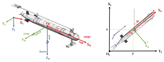
Figure 4.
The inertia coordinate is OI-XIYIZI, and the body coordinate is OB-XBYBZB. The translation and rotation motions are indicated along each axis.
3.2. Dynamic Modeling
Based on the Newton–Euler motion equations for a rigid body in fluid and AUV model proposed by Fossen [30], the vector representation method of the dynamic model is as follows:
where M represents the inertia matrix, incorporating added mass, C is the Coriolis and centripetal force matrix of the underwater robot, D is the fluid resistance matrix of the underwater robot, g denotes the restoring force (torque) vector generated by gravity and buoyancy, while τ is the force (torque) vector produced by the propeller.
Combining the representation methods of kinematics and dynamics [31,32], ignoring the couplings between degrees of freedom, the SSOP model can be expressed as Equation (4).
Based on the longitudinal and yaw two-degree-of-freedom dynamic model as the foundational framework, this study achieves optimal trajectory tracking control by integrating the Line-of-Sight (LOS) guidance method with the Model Predictive Control (MPC) algorithm. The pitch degree-of-freedom control is uniquely addressed through a model-independent dual-loop PID controller, thereby reducing the original system dynamics model to the simplified form presented in Equation (5). This architecture not only streamlines the model structure through algorithmic integration but also substantially alleviates the computational load of the LOS-MPC integrated controller described in Section 4 by decoupling the pitch-loop control, ultimately ensuring the system’s real-time performance.
3.3. Model Parameters Identification
Generally, the parameter identification of the underwater vehicle dynamic model involves various methods. These include the least squares method, maximum likelihood estimation, extended Kalman filter, and adaptive identification techniques. The dynamic model is a nonlinear equation with linear parameters, so it is reasonable to choose the least squares identification parameters [33]. The reason why this method is used for identification is that it can provide the consistency of parameter estimation, high robustness, and high fitting when processing the measured data of a noisy submersible. Compared to other methods, such as the extended Kalman filter (EKF), the least squares method offers several advantages. First, it is well-suited for handling nonlinear models with linear parameters and is computationally efficient, making it suitable for real-time applications. Additionally, it has strong robustness to noise, providing consistent and accurate parameter estimates with high fitting quality. In contrast, EKF requires more complex noise modeling and incurs higher computational costs. Therefore, the least squares method provides a simpler and more stable solution for parameter identification in SSOP dynamic modeling.
Before identifying the parameters of the dynamic model, the linear uniform experiment was designed to obtain the data on SSOP velocity and thrust, and the in situ rotation uniform circle experiment was designed to obtain the data on SSOP angular velocity and torque. Based on the data information obtained from the investigation, the unidentified coefficients of the dynamic model are obtained through the following identification process.
Assume that the system model to be identified is the following:
In Equation (6), t is time, is the observation vector, is the time-varying vector, and represents the model parameter vector that requires estimation. The least squares estimation of the parameter is:
Two single-degree-of-freedom models of the SSOP are obtained by identifying the model and the parameters in Equation (5) with the above classical least squares method.
4. LOS-MPC-Based Path Following Controller
4.1. System Controller for the Path Following
The system controller for path following is depicted in Figure 5. The controller consists of the LOS and the MPC controller. The LOS part calculates the expected heading angle according to the predicted trajectory point in real time. The MPC controller tracks the anticipated heading angle provided by LOS. Additionally, throughout this procedure, the practical limitations can be replicated in actual applications. The linearized predictive framework derived from state-space representation, the objective function, as well as the control strategies, must be formulated to develop the MPC controller. The subsequent subsections will provide specific designs for LOS and MPC controllers.
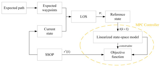
Figure 5.
System architecture of the SSOP.
4.2. LOS Tracking Method
The Line-of-Sight (LOS) method is a technique used to calculate the LOS angle, which can determine the desired heading angle in real time for an Autonomous Underwater Vehicle (AUV) to achieve path following. The selected path is a geometric path parameterized by arc length and consists of reference waypoints depicted in Figure 6. It is assumed that there is a circle with the center at the tracked reference waypoint with the Optimal Bayesian Filter Navigation (SSOP), and the radius is R. The criterion for selecting the next path point is that the current horizontal position of the AUV at a certain moment satisfies Equation (8). In Equation (8), R is typically chosen as 2–5 times the length of the AUV.
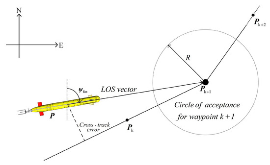
Figure 6.
Schematic diagram of LOS path following.
In this paper, the current position in the inertial coordinate system is obtained through inertial navigation. Assuming that the desired position for path following is denoted as , and the current actual position is . Then, the LOS angle is calculated using Equation (9).
4.3. Controller Based on MPC
The frame of a typical MPC controller contains three parts, which are the predictive model, the objective function, and rolling optimization. For the tracking control, the linear MPC is designed. The diagram of the proposed linear MPC controller is depicted in Figure 5. The linear MPC regulator can adjust the control command based on both the robot’s present condition and the anticipated future state deviation. Moreover, throughout this procedure, real-world constraints can be incorporated into practical implementation. The predictive model based on linear state space, along with the objective function and rules, must be established to develop a controller.
4.3.1. Linearized State-Space-Based Predictive Model of SSOP
The predictive model for state tracking is formulated with Equation (10) according to Equation (4) to obtain the control signal according to the target state.
where , , and , the matrices and in Equation (10) are presented as follows:
It is readily observed that the aforementioned state-space formulation is nonlinear. It is crucial to linearize Equation (10) to create an MPC approach based on state-space representation. Each point on the reference trajectory satisfies the above state-space equation, where the subscript d represents the reference. The general form is expressed as follows:
where is the desired state, and is the corresponding control value. The Taylor series expansion at the reference point is utilized in the Equation (10), and high-order terms are neglected to derive the following equation:
The SSOP linearized error model is derived from the difference between Equations (14) and (13).
where , and .
The model in Equation (15) is the continuous-time model. In order to apply the model to the SSOP plant, the approximate discrete method is used to discretize Formula (15). The discretized form of Equation (15) is expressed as follows:
where , , is an identity matrix, and is the sampling time of the SSOP system.
4.3.2. Design of the Optimization Function for the State Tracking of SSOP
Defining a suitable optimization objective is crucial for accurately tracking the desired state. In addition, the value of the control input should be as small as possible to save energy. A relaxation factor is formulated and incorporated into the objective function to avoid degeneracy. According to the above rules, the objective function is organized as follows:
where , , and are the weighting matrices, is the prediction horizon, and is the control horizon. is a weighting factor. is the relaxing factor. Therefore, the optimization problem of Model Predictive Controllers can be described as follows:
where and are the limit value of the control input.
4.3.3. Solution to the Proposed Algorithm
The optimization framework defined in Equation (18) is transformed into a quadratic programming (QP) formulation, incorporating the constraints outlined below:
where , , , . The matrix in the definition of H, and the matrix in the definition of G are expressed as follows:
The above standard quadratic optimization problem obtains the control input sequence in the control time domain and can be expressed as Equation (20). Within this sequence of control actions, the initial component is applied to the robot system.
5. Experiments and Analysis
5.1. The Prototype of SSOP
The SSOP platform utilized in this study is illustrated in Figure 7, with its specific characteristics provided in Table 1. The robot has dimensions of 5.9 m in length, 5.5 m in width, and 6.6 m in height when the antenna is raised, with a total weight of 920 kg. During underwater exploration missions, such as seafloor resource exploration or target searching, the robot can operate at a maximum depth of 10 m. The SSOP has a maximum speed of 6 knots, and with the embedded positioning system, the dead-reckoning error is less than 3‰ of the travel distance. The robot can continuously navigate for 40 h at a speed of 3 knots and for 12 h at a speed of 6 knots.
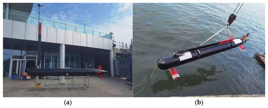
Figure 7.
The SSOP prototype.(a) SSOP antenna deployed; (b) SSOP layout diagram.

Table 1.
Mechanical details of the SSOP prototype.
5.2. Ocean Experimental Setup
The SSOP mentioned in this paper has been experimentally verified across several performance metrics, including maximum speed, navigation accuracy, maximum operating depth, continuous operation time, and terrain exploration capability. In this study, an SSOP was used for underwater motion control experiments. The experimental site is located in the southern offshore waters of the National Marine Comprehensive Test Site (Weihai), as indicated by the positioning marker in Figure 8a. Figure 8b illustrates the motion process of the SSOP during the sea trial.
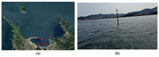
Figure 8.
Experimental scene. (a) Location of the experimental sea area; (b) Antenna above water during sea trial.
5.3. System Identification Results and Verification
To identify the dynamic model parameters of the SSOP, it is necessary to first obtain the state information of the submersible. To this end, an inertial navigation system (INS) and a DVL are installed on the SSOP to collect relevant data. In Figure 9, the data collected by the sensors are transmitted to the main control compartment via serial communication. The navigation board in the main control compartment parses and packages the data before sending it to the sensor board. The sensor board then fuses the received data with other information, repackages it, and sends it to the main control board. Subsequently, the primary control module transmits the state information of the SSOP to the ground station via the 4G antenna of the communication and positioning system. At the same time, commands from the ground station are transmitted to the central controller via the 4G link. The central controller adjusts the PWM signals to effectively control the main thruster and rudders.
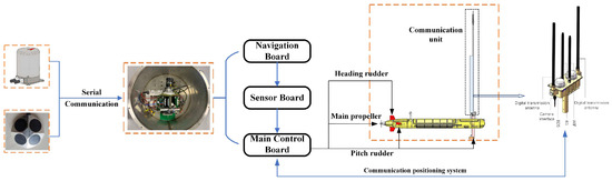
Figure 9.
Identification data acquisition flow chart: sensor data real-time acquisition and control instructions issued.
Using the aforementioned control methods, we designed linear uniform motion experiments and uniform circular motion experiments with in situ rotation, with each set of experiments being repeated three times. Finally, the dynamic model parameters were identified using the least squares method described in Section 3.3. During the experiments, different data intervals were selected multiple times to obtain the most accurate dynamic model of the SSOP, and the result with the smallest Root Mean Square Error (RMSE) was chosen as the final model. The final model results for the longitudinal and yaw degrees of freedom of the SSOP are as follows:
We analyzed and compared the fitting results of the aforementioned models with the actual values in Figure 10. Firstly, the pre-acquired data were substituted into the left-hand side of Equation (8) to calculate the model-predicted thrust and torque. Then, the calculated values were compared with the actual values. Figure 10a shows the comparison results between the calculated and actual values of thrust, whereas Figure 10b shows the analogous data between the calculated and actual values of torque. As observed in Figure 10, the identified model fits the actual values very well.
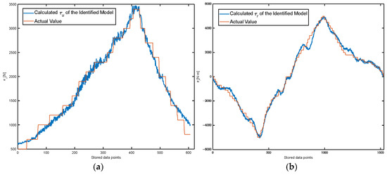
Figure 10.
Comparison between identification results and ground truth. (a) The comparison result between the identified thrust and the ground truth. (b) The comparison result between the identified torque and the ground truth.
5.4. Directional Control Experiments
To assess the actual heading performance of the SSOP, heading tests are carried out in a marine environment with a wind force of 4 and a wave height of 0.8 m. Since the initial heading of the SSOP is unknown in practical applications, we specifically simulated scenarios where the initial heading angle was significantly different from the desired heading angle. In the tests, the initial headings of the SSOP were 20.7°, 34.8°, and 36.4°, respectively, while the desired heading was 45°. Figure 11 shows the heading results of the SSOP, with the lower graph illustrating the heading convergence. The experimental results indicate that the final heading accuracy error was 2°. Despite the large deviation of the initial heading from the desired heading angle, the SSOP was able to quickly adjust its yaw angle and eventually stabilize at the desired heading. This demonstrates that the proposed MPC controller exhibits fast convergence and tracking performance.
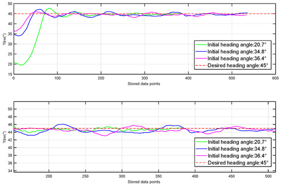
Figure 11.
Experimental results of the heading angle.
5.5. “8”-Type Path Following Experiments
To assess the performance of the previously introduced LOS-MPC method, sea trials for “figure-eight” trajectory tracking were conducted at the Weihai Test Site (Figure 8). The equation for the “figure-eight” trajectory is shown in Equation (22), where the parameter a is 150, resulting in a lateral extent of 300 m and a longitudinal extent of 106 m for the trajectory.
During the testing process, the high-precision GPS/INS inertial navigation system outputs the position information and attitude of the SSOP, including latitude, longitude, heading angle, and angular velocity. This data is transmitted to the ground control terminal via 4G communication at a frequency of 10 Hz. The ground terminal inputs the received SSOP state data into the LOS-MPC controller, which calculates the optimal thrust and torque and then sends these values back to the SSOP through the same communication link. Upon receiving the control commands, the communication and positioning module forwards them to the main controller for resolution and thrust allocation, which are ultimately applied to the main propulsion motor, pitch rudder, and yaw rudder.
Figure 12 shows a photo of the SSOP navigating along the “figure-eight” trajectory during the offshore sea trial. The trajectory tracking diagram of the SSOP’s upper computer is shown in Figure 13, where the red dots represent 32 preset trajectory points that constitute the predicted trajectory. The SSOP achieves trajectory tracking by following these points sequentially. Determined by whether the separation between the current position and the target position is less than three times the SSOP’s length, the control system can make real-time judgments on whether to switch to the next desired point.
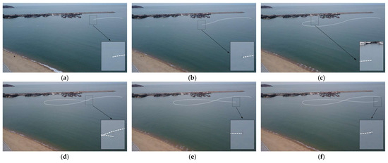
Figure 12.
The snapshot of the SSOP in the “8” path following experiment. (a) t = 128 s. (b) t = 251 s. (c) t = 416 s. (d) t = 536 s. (e) t = 636 s. (f) t = 688 s.
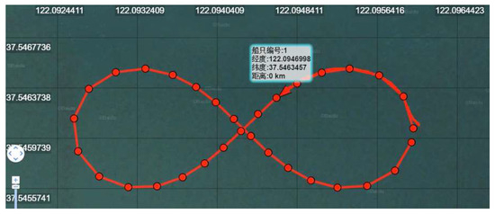
Figure 13.
“8”-type path following effect diagram. (The figure displays the SSOP serial numbers along with their latitude and longitude coordinates).
To demonstrate the superiority of the proposed LOS-MPC algorithm, this paper conducted comparative experiments with the traditional PID algorithm. Both algorithms were tested with the same desired trajectory, and to verify their disturbance rejection capabilities, comparative tests were also performed under adverse sea conditions. On the day of the sea trial, the sea conditions were characterized by a wind force of 4 and wave heights of 1 m. The comparative findings are illustrated in Figure 14. The LOS-MPC algorithm outperforms the PID algorithm in stability, reliability, and resistance to water currents. MPC’s model-based optimization dynamically adjusts control actions, counteracting flow disturbances more effectively than the fixed-gain PID controller. In contrast, PID often exhibits severe oscillations when facing currents due to overcompensation. By proactively optimizing control inputs, MPC ensures smoother and more stable trajectory tracking. Figure 15 illustrates the tracking errors of the two algorithms. The results indicate that even under time-varying sea conditions, the LOS-MPC algorithm can still maintain the effectiveness of path tracking, keeping the error between the SSOP and the desired point within 3 m.
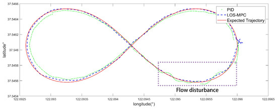
Figure 14.
Path following Results of the PID and the proposed LOS-MPC method.
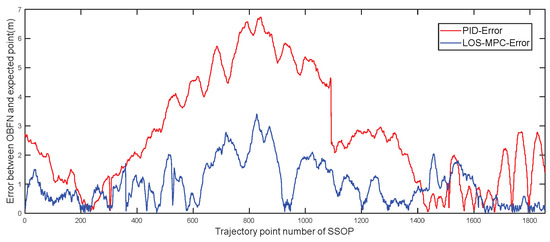
Figure 15.
Path following errors of PID and the proposed LOS-MPC method.
Under identical maritime experimental conditions and shared desired trajectories, the LOS-MPC significantly outperforms the conventional PID method in trajectory tracking for SSOP applications. LOS-MPC reduces the average position error by 59% compared to PID, with maximum and minimum errors reduced to 51% and 15% of PID’s values, respectively. The substantially lower Mean Squared Error (MSE) and tighter error bounds validate LOS-MPC’s enhanced robustness against extreme disturbances and steady-state conditions. As demonstrated in Figure 15 and Table 2, LOS-MPC achieves superior accuracy and stability in dynamic marine environments through real-time rolling optimization, effectively addressing multivariable coupling and system constraints. These results position LOS-MPC as a high-precision alternative to PID for SSOP trajectory control.
Table 2.
Experimental Results of Different Methods.
6. Conclusions
To address the path-tracking challenge of the SSOP under disturbances, this paper designs a real-time MPC strategy based on the LOS method. By integrating the kinematic and dynamic models of the SSOP and utilizing its previously recorded motion data, a more accurate predictive model is identified. This enables the improved LOS-MPC approach to track the desired trajectory more precisely. We also conducted ocean experiments and compared the improved LOS-MPC with traditional algorithms. The results demonstrate that the proposed method exhibits high effectiveness and robustness in path tracking, capable of quickly driving the SSOP to accurately follow the reference path. The future work of this research will further explore multi-source disturbance modeling and compensation, multi-objective optimization and collaborative control, real-time performance optimization, and long-term experimental validation. Through in-depth investigation of these directions, the findings of this study will be further refined, providing enhanced technical support for the autonomous navigation and control of the SSOP and other marine equipment, thereby advancing the intelligent development of marine engineering.
Author Contributions
Conceptualization was led by S.W., X.Y. and S.W. designed the methodology and developed the software in collaboration with R.Z. Experimental validation and formal analysis were jointly conducted by S.W., X.Y. and M.L., with technical investigations performed by S.W., R.Z. and X.Y. provided critical resources and secured funding for the research. S.W. curated the datasets and drafted the original manuscript. R.Z. contributed to data visualization and graphical representations. Manuscript review and editing were collaboratively undertaken by S.W. and X.Y. Project administration was managed by S.W. and M.L., while S.W. supervised the overall research workflow. All authors have read and agreed to the published version of the manuscript.
Funding
This work was supported by the Laoshan laboratory science and technology innovation project (LSKJ202205500) and the National Natural Science Foundation of China (Grant No. 42276187).
Data Availability Statement
The data presented in this study are available on request from the corresponding author.
Conflicts of Interest
The authors declare no conflicts of interest.
References
- Tang, Z.; Cao, X.; Zhou, Z.; Zhang, Z.; Xu, C.; Dou, J. Path Planning of Autonomous Underwater Vehicle in Unknown Environment Based on Improved Deep Reinforcement Learning. Ocean. Eng. 2024, 301, 117547. [Google Scholar] [CrossRef]
- Firat, E.; Shachak, P.; May-Win, T.; Yuri, R.; Barbaros, C.; Swift, M. Position, Orientation and Velocity Detection of Unmanned Underwater Vehicles (UUVs) Using an Optical Detector Array. Sensors 2017, 17, 1741. [Google Scholar] [CrossRef] [PubMed]
- He, Y.; Zhu, L.; Sun, G.; Qiao, J.; Guo, S. Underwater Motion Characteristics Evaluation of Multi Amphibious Spherical Robots. Microsyst. Technol. 2019, 25, 499–508. [Google Scholar]
- Du, S.; Wu, Z.; Yu, J. Design and Yaw Control of a Two-Motor-Actuated Biomimetic Robotic Fish. In Proceedings of the 2019 IEEE International Conference on Robotics and Biomimetics (ROBIO), Dali, China, 6–8 December 2019; pp. 126–131. [Google Scholar]
- Wu, Z.; Yu, J.; Yuan, J.; Tan, M. Towards a Gliding Robotic Dolphin: Design, Modeling, and Experiments. IEEE/ASME Trans. Mechatron. 2019, 24, 260–270. [Google Scholar] [CrossRef]
- Wang, S.; Wang, Y.; Wei, Q.; Tan, M.; Yu, J. A Bio-Inspired Robot With Undulatory Fins and Its Control Methods. IEEE/ASME Trans. Mechatron. 2017, 22, 206–216. [Google Scholar]
- Chen, Y.; Yuan, L.; Qin, L.; Zhang, N.; Li, L.; Wu, K.; Zhou, Z. A Forecasting Model with Hybrid Bidirectional Long Short-Term Memory for Mooring Line Responses of Semi-Submersible Offshore Platforms. Appl. Ocean. Res. 2024, 150, 104145. [Google Scholar] [CrossRef]
- Gu, H.; Chen, H.-C. Numerical Simulation of a Semi-Submersible FOWT Platform under Calibrated Extreme and Irregular Waves. Ocean. Eng. 2024, 311, 118847. [Google Scholar] [CrossRef]
- Degorre, L.; Fossen, T.I.; Delaleau, E.; Chocron, O. A Virtual Reference Point Kinematic Guidance Law for 3-D Path-Following of Autonomous Underwater Vehicles. IEEE Access 2024, 12, 109822–109831. [Google Scholar] [CrossRef]
- Jia, H.M.; Zhang, L.J.; Cheng, X.Q.; Bian, X.Q.; Zhou, J.J. Three-Dimensional Path Following Control for an Underactuated UUV Based on Nonlinear Iterative Sliding Mode. Acta Autom. Sin. 2012, 38, 308–314. [Google Scholar]
- Elmokadem, T.; Zribi, M.; Youcef-Toumi, K. Trajectory Tracking Sliding Mode Control of Underactuated AUVs. Nonlinear Dyn. 2016, 84, 1079–1091. [Google Scholar]
- Elmokadem, T.; Zribi, M.; Youcef-Toumi, K. Terminal Sliding Mode Control for the Trajectory Tracking of Underactuated Autonomous Underwater Vehicles. Ocean. Eng. 2016, 129, S0029801816304759. [Google Scholar]
- Soylu, S.; Proctor, A.A.; Podhorodeski, R.P.; Bradley, C.; Buckham, B.J. Precise Trajectory Control for an Inspection Class ROV. Ocean. Eng. 2016, 111, 508–523. [Google Scholar]
- Soylu, S.; Buckham, B.J.; Podhorodeski, R.P. A Chattering-Free Sliding-Mode Controller for Underwater Vehicles with Fault-Tolerant Infinity-Norm Thrust Allocation. Ocean. Eng. 2008, 35, 1647–1659. [Google Scholar]
- Pan, C.Z.; Lai, X.Z.; Yang, S.X.; Wu, M. An Efficient Neural Network Approach to Tracking Control of an Autonomous Surface Vehicle with Unknown Dynamics. Expert Syst. Appl. Int. J. 2013, 40, 1629–1635. [Google Scholar]
- Miao, B.; Li, T.; Luo, W. A DSC and MLP Based Robust Adaptive NN Tracking Control for Underwater Vehicle. Neurocomputing 2013, 111, 184–189. [Google Scholar] [CrossRef]
- Hu, Z.; Zhu, D.; Cui, C.; Sun, B. Trajectory Tracking and Re-Planning with Model Predictive Control of Autonomous Underwater Vehicles. J. Navig. 2018, 72, 321–341. [Google Scholar] [CrossRef]
- Sun, B.; Zhu, D.; Yang, S.X. A Bioinspired Filtered Backstepping Tracking Control of 7000-m Manned Submarine Vehicle. IEEE Trans. Ind. Electron. 2014, 61, 3682–3693. [Google Scholar]
- Liu, G.; Mo, C.; Wei, S.; Zhang, Y. Energy Consumption Optimization Strategy for Autonomous Underwater Vehicles Based on Model Prediction Control. In Proceedings of the 2024 IEEE 7th Advanced Information Technology, Electronic and Automation Control Conference (IAEAC), Chongqing, China, 15–17 March 2024; Volume 7, pp. 17–21. [Google Scholar]
- Shen, C.; Shi, Y.; Buckham, B. Integrated Path Planning and Tracking Control of an AUV: A Unified Receding Horizon Optimization Approach. IEEE/ASME Trans. Mechatron. 2017, 22, 1163–1173. [Google Scholar]
- Shen, C.; Buckham, B.; Shi, Y. Modified C/GMRES Algorithm for Fast Nonlinear Model Predictive Tracking Control of AUVs. IEEE Trans. Control. Syst. Technol. 2016, 25, 1896–1904. [Google Scholar]
- Shen, C.; Shi, Y.; Buckham, B. Trajectory Tracking Control of an Autonomous Underwater Vehicle Using Lyapunov-Based Model Predictive Control. IEEE Trans. Ind. Electron. 2017, 65, 5796–5805. [Google Scholar]
- Shen, C.; Shi, Y. Distributed Implementation of Nonlinear Model Predictive Control for AUV Trajectory Tracking. Automatica 2020, 115, 108863. [Google Scholar] [CrossRef]
- Xue, Y.; Wang, X.; Liu, Y.; Xue, G. Real-Time Nonlinear Model Predictive Control of Unmanned Surface Vehicles for Trajectory Tracking and Collision Avoidance. In Proceedings of the 2021 7th International Conference on Mechatronics and Robotics Engineering, ICMRE 2021, Budapest, Hungary, 3–5 February 2021; pp. 150–155. [Google Scholar] [CrossRef]
- Bhat, S.; Panteli, C.; Stenius, I.; Dimarogonas, D.V. Nonlinear Model Predictive Control for Hydrobatics: Experiments with an Underactuated AUV. J. Field Robot. 2023, 40, 1840–1859. [Google Scholar] [CrossRef]
- Zhao, D.; Gao, S.; Spurgeon, S.K.; Reichhartinger, M. Adaptive Sliding Mode Dynamic Positioning Control for a Semi-Submersible Offshore Platform. In Proceedings of the 2019 18th European Control Conference (ECC), Naples, Italy, 25–28 June 2019; IEEE: Naples, Italy, 2019; pp. 3103–3108. [Google Scholar]
- Kang, S.; Yu, J.; Zhang, J.; Hu, F.; Jin, Q. Research on Accurate Modeling of Hydrodynamic Interaction Forces on AUVs Operating in Tandem. Ocean. Eng. 2022, 251, 111125. [Google Scholar] [CrossRef]
- Sajedi, Y.; Bozorg, M. Robust Estimation of Hydrodynamic Coefficients of an AUV Using Kalman and H∞ Filters. Ocean. Eng. 2019, 182, 386–394. [Google Scholar] [CrossRef]
- Valluru, S.K.; Thareia, H. Maneuvering Control of Autonomous Underwater Vehicle (AUV) by Simulated Annealing and Moth Flame Optimization Tuned Controllers. In Proceedings of the 2022 International Conference on Electronic Systems and Intelligent Computing (ICESIC), Chennai, India, 22–23 April 2022; pp. 223–228. [Google Scholar]
- Källström, C.G. Guidance and Control of Ocean Vehicles; Fossen, T.I., Ed.; Wiley: Chichester, UK, 1996; Volume 32, p. 1235. ISBN 0-471-94113-1. [Google Scholar] [CrossRef]
- Du, P.; Ouahsine, A.; Toan, K.T.; Sergent, P. Simulation of Ship Maneuvering in a Confined Waterway Using a Nonlinear Model Based on Optimization Techniques. Ocean. Eng. 2017, 142, 194–203. [Google Scholar] [CrossRef]
- Tran Khanh, T.; Ouahsine, A.; Naceur, H.; El Wassifi, K. Assessment of Ship Manoeuvrability by Using a Coupling between a Nonlinear Transient Manoeuvring Model and Mathematical Programming Techniques. J. Hydrodyn. 2013, 25, 788–804. [Google Scholar] [CrossRef]
- Huang, J.; Zhang, Y.; Yang, X.; Luo, Z. Transfer Function Model Identification Based on Improved Least Square Method. In Proceedings of the 2020 Chinese Automation Congress (CAC), Shanghai, China, 6–8 November 2020; pp. 487–491. [Google Scholar]
Disclaimer/Publisher’s Note: The statements, opinions and data contained in all publications are solely those of the individual author(s) and contributor(s) and not of MDPI and/or the editor(s). MDPI and/or the editor(s) disclaim responsibility for any injury to people or property resulting from any ideas, methods, instructions or products referred to in the content. |
© 2025 by the authors. Licensee MDPI, Basel, Switzerland. This article is an open access article distributed under the terms and conditions of the Creative Commons Attribution (CC BY) license (https://creativecommons.org/licenses/by/4.0/).