
Surface Current Observations in the Southeastern Tropical Indian Ocean Using Drifters


Abstract
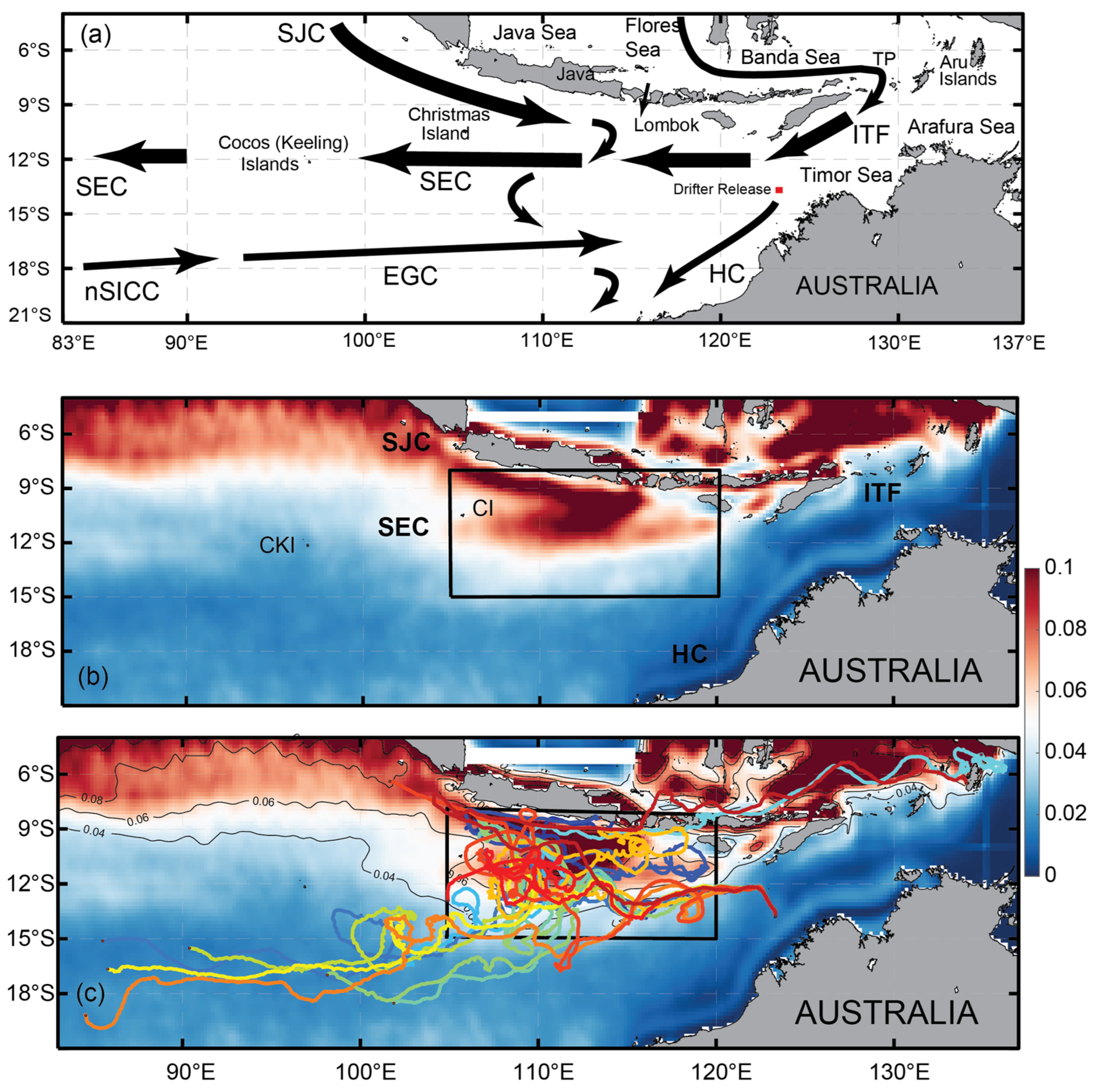
1. Introduction
2. Methodology
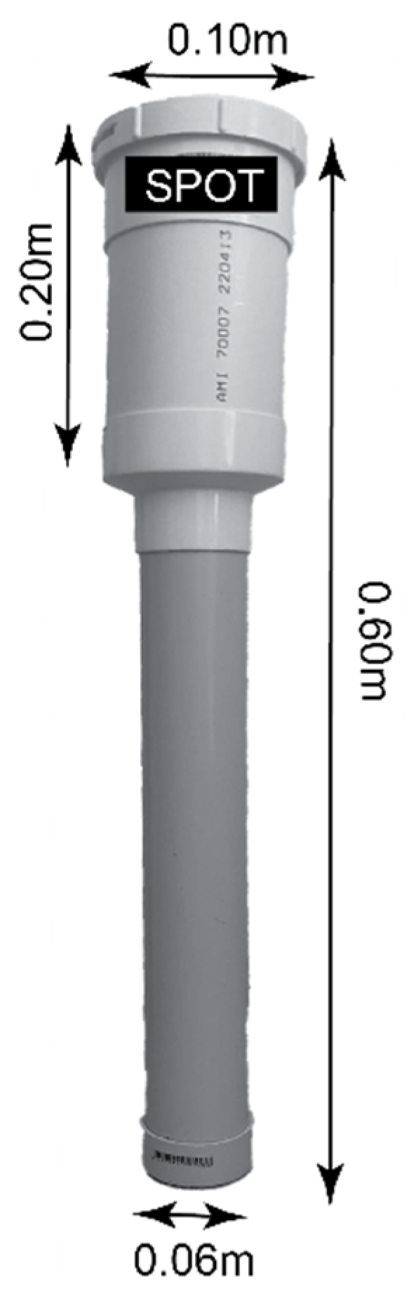
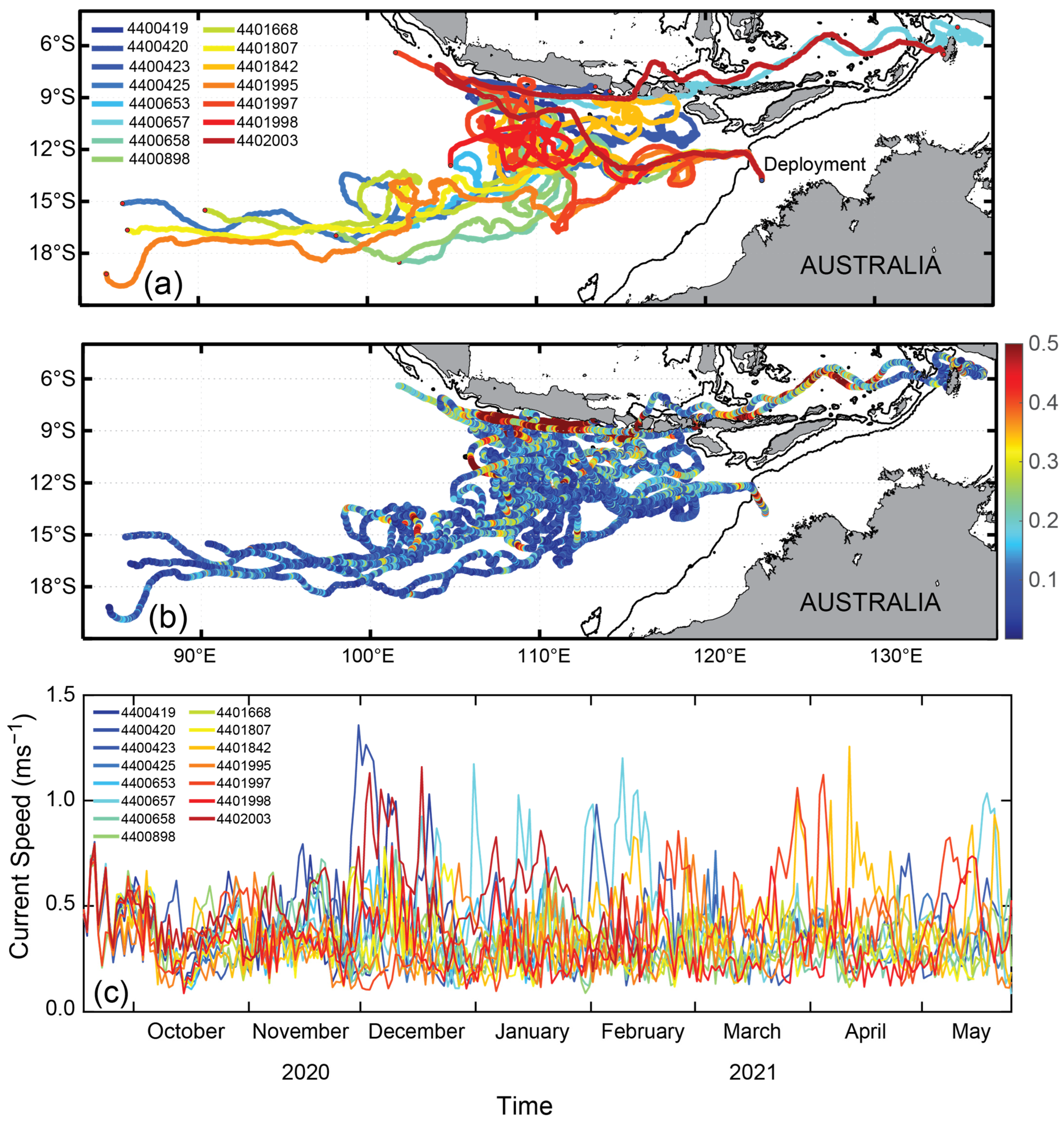
2.1. The Surface Drifters
2.2. Analytical Approaches
2.2.1. Outlier Removal
2.2.2. Spectral Analysis and Wavelet Analysis
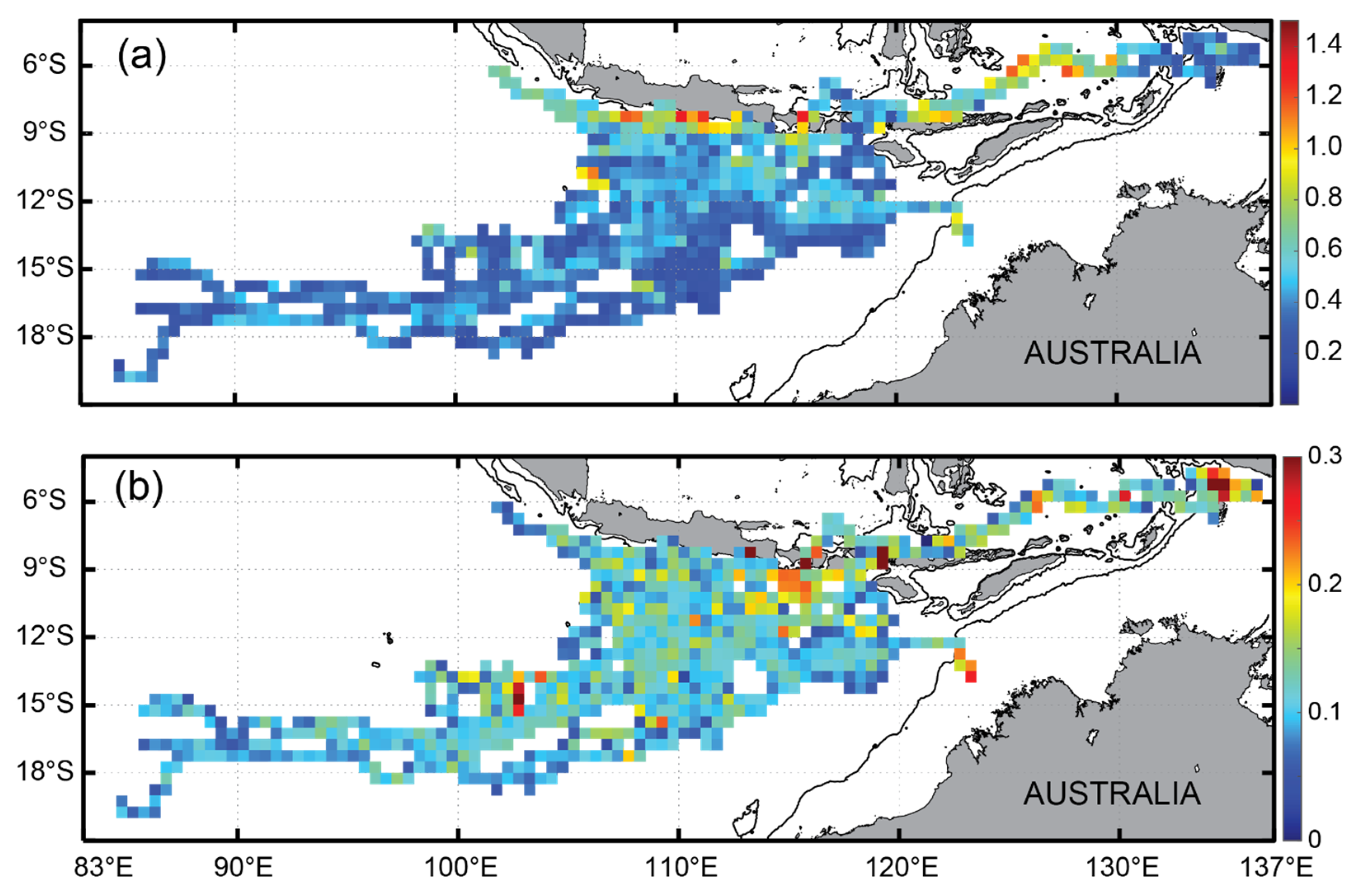
2.3. Kinetic Energy and Eddy Kinetic Energy
3. Results
3.1. Forcing Mechanisms of Surface Currents
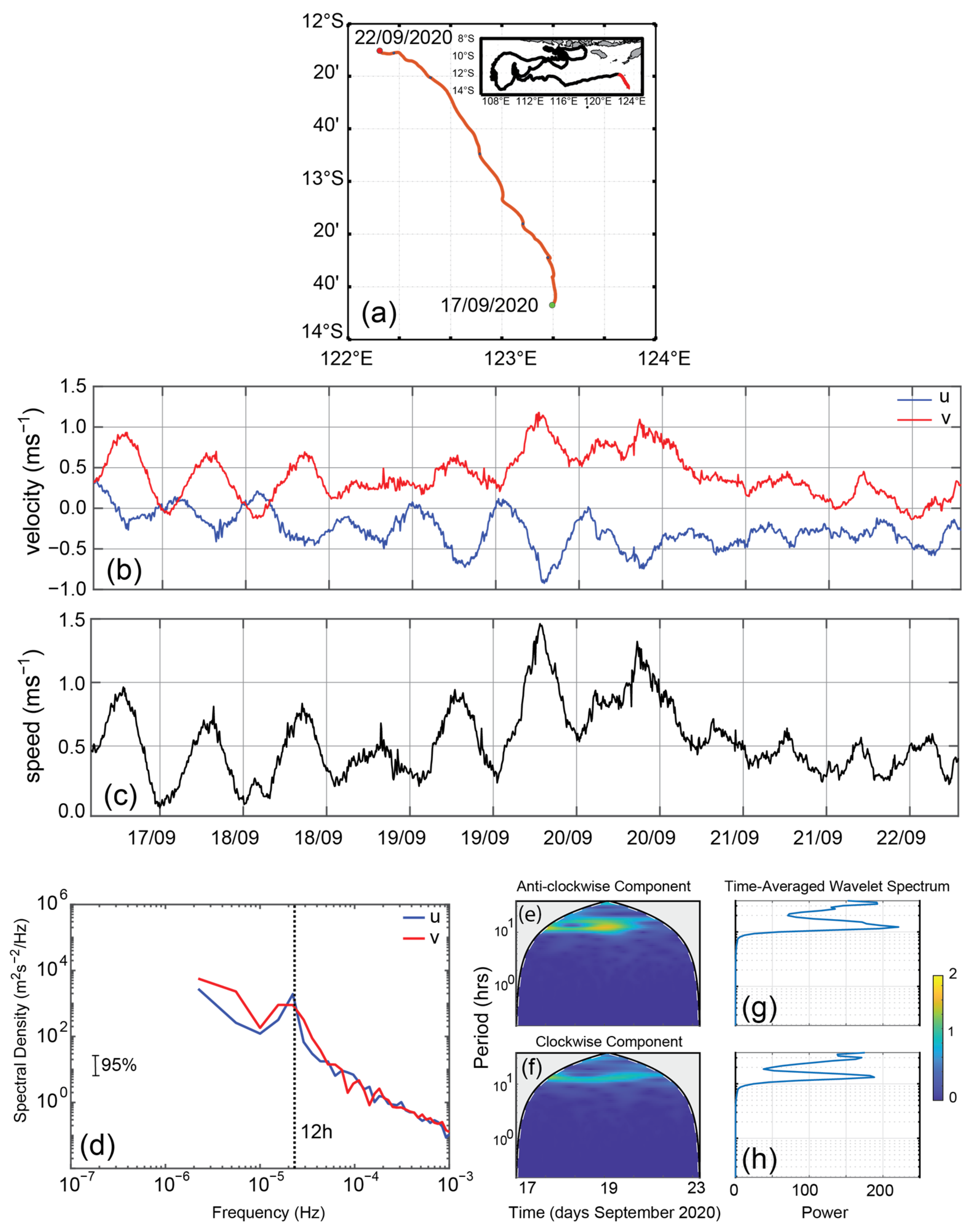
3.1.1. Semidiurnal Tides
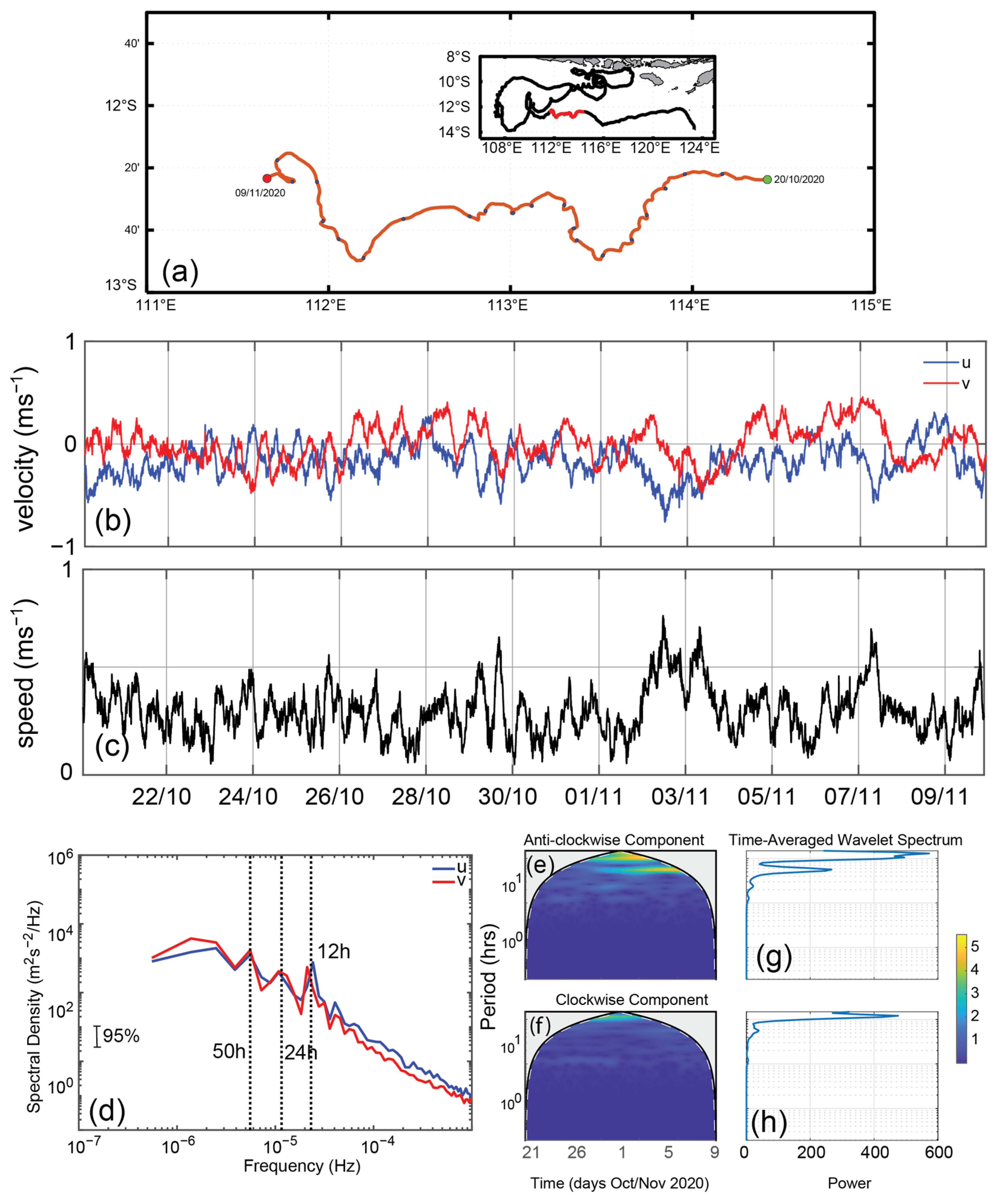
3.1.2. Mixed Forcing: Inertial, Semi-Diurnal, and Diurnal Tides
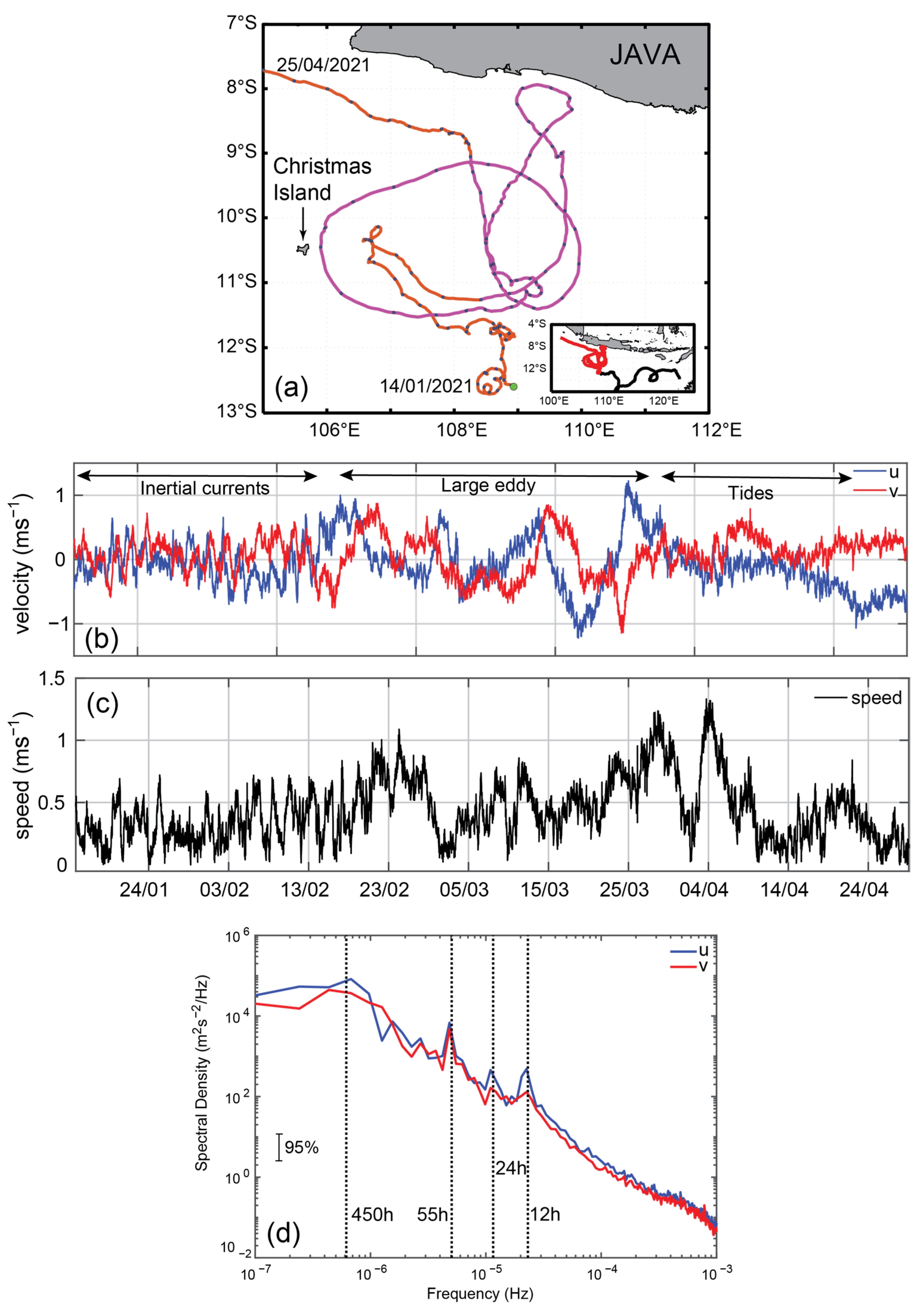
3.1.3. Mesoscale Eddy
3.1.4. Strait Flow
3.1.5. Headland Flow—Diurnal Tidal Currents
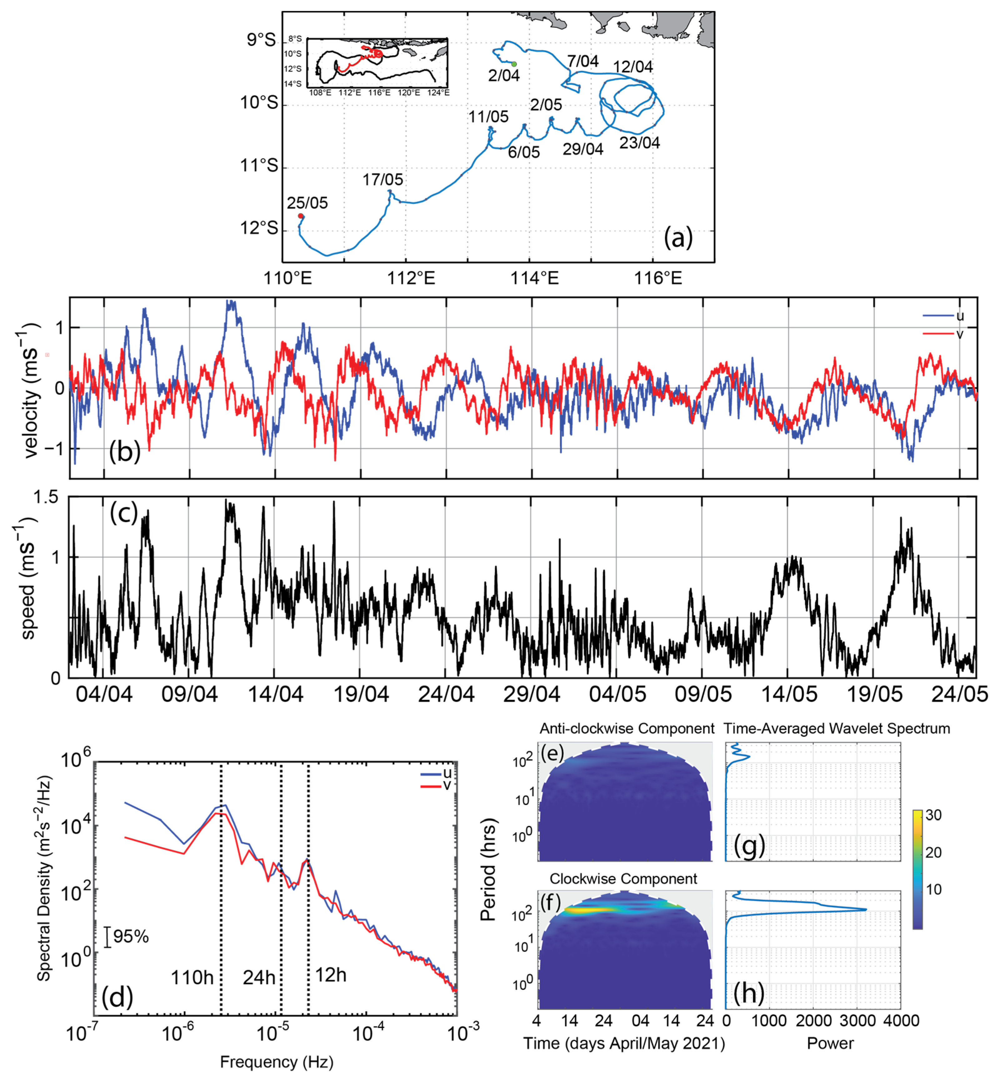
3.1.6. Inertial Currents from a Tropical Storm
4. Discussion
5. Conclusions
Author Contributions
Funding
Informed Consent Statement
Data Availability Statement
Acknowledgments
Conflicts of Interest
References
- Siegel, D.A.; Kinlan, B.P.; Gaylord, B.; Gaines, S.D. Lagrangian descriptions of marine larval dispersion. Mar. Ecol. Prog. Ser. 2003, 260, 83–96. [Google Scholar] [CrossRef]
- Pattiaratchi, C.; van der Mheen, M.; Schlundt, C.; Narayanaswamy, B.E.; Sura, A.; Hajbane, S.; White, R.; Kumar, N.; Fernandes, M.; Wijeratne, S. Plastics in the Indian Ocean–sources, transport, distribution, and impacts. Ocean Sci. 2022, 18, 1–28. [Google Scholar]
- Azis Ismail, M.F.; Ribbe, J.; Arifin, T.; Taofiqurohman, A.; Anggoro, D. A census of eddies in the tropical eastern boundary of the Indian Ocean. J. Geophys. Res. Ocean. 2021, 126, e2021JC017204. [Google Scholar] [CrossRef]
- Feng, M.; Zhang, N.N.; Liu, Q.Y.; Wijffels, S. The Indonesian throughflow, its variability and centennial change. Geosci. Lett. 2018, 5, 3. [Google Scholar] [CrossRef]
- Guo, Y.; Li, Y.; Cheng, L.; Chen, G.; Liu, Q.; Tian, T. An updated estimate of the Indonesian Throughflow geostrophic transport: Interannual variability and salinity effect. Geophys. Res. Lett. 2023, 50, e2023GL103748. [Google Scholar] [CrossRef]
- Broecker, W.S. The great ocean conveyor. Oceanography 1991, 4, 79–89. [Google Scholar] [CrossRef]
- Gordon, A.L.; Fine, R.A. Pathways of water between the Pacific and Indian oceans in the Indonesian seas. Nature 1996, 379, 146–149. [Google Scholar] [CrossRef]
- Qu, T.; Meyers, G. Seasonal characteristics of circulation in the southeastern tropical Indian Ocean. J. Phys. Ocean. 2005, 35, 255–267. [Google Scholar]
- Schott, F.A.; Xie, S.P.; McCreary, J.P., Jr. Indian Ocean circulation and climate variability. Rev. Geophys. 2009, 47, RG1002. [Google Scholar]
- Sprintall, J.; Gordon, A.L.; Koch-Larrouy, A.; Lee, T.; Potemra, J.T.; Pujiana, K.; Wijffels, S.E. The Indonesian seas and their role in the coupled ocean–climate system. Nat. Geosci. 2014, 7, 487–492. [Google Scholar]
- Chen, G.; Han, W.; Wang, D.; Zhang, L.; Chu, X.; He, Y.; Chen, J. Seasonal structure and interannual variation of the South Equatorial Current in the Indian Ocean. J. Geophys. Res. Ocean. 2022, 127, e2022JC018969. [Google Scholar] [CrossRef]
- Gruenburg, L.K.; Gordon, A.L.; Thurnherr, A.M. Indonesian Throughflow partitioning between Leeuwin and south equatorial currents. J. Phys. Ocean. 2023, 53, 2159–2170. [Google Scholar] [CrossRef]
- Saji, N.H.; Goswami, B.N.; Vinayachandran, P.N.; Yamagata, T. A dipole mode in the tropical Indian Ocean. Nature 1999, 401, 360–363. [Google Scholar] [CrossRef] [PubMed]
- Meyers, G.; McIntosh, P.; Pigot, L.; Pook, M. The years of El Niño, La Niña, and interactions with the tropical Indian Ocean. J. Clim. 2007, 20, 2872–2880. [Google Scholar] [CrossRef]
- Chen, G.; Wang, D.; Han, W.; Feng, M.; Wang, F.; Li, Y.; Chen, J.; Gordon, A.L. The extreme El Niño events suppressing the intraseasonal variability in the eastern tropical Indian Ocean. J. Phys. Ocean. 2020, 50, 2359–2372. [Google Scholar] [CrossRef]
- Chen, G.; Han, W.; Li, Y.; Wang, D. Interannual variability of equatorial eastern Indian Ocean upwelling: Local versus remote forcing. J. Phys. Ocean. 2016, 46, 789–807. [Google Scholar] [CrossRef]
- Telcik, N.; Pattiaratchi, C. Influence of northwest cloud bands on southwest Australian rainfall. J. Climatol. 2014, 2014, 671394. [Google Scholar] [CrossRef]
- Honda, K.; Hobday, A.J.; Kawabe, R.; Tojo, N.; Fujioka, K.; Takao, Y.; Miyashita, K. Age-dependent distribution of juvenile southern bluefin tuna (Thunnus maccoyii) on the continental shelf off southwest Australia determined by acoustic monitoring. Fish. Oceanog. 2010, 19, 151–158. [Google Scholar] [CrossRef]
- Tussadiah, A.; Pranowo, W.S.; Syamsuddin, M.L.; Riyantini, I.; Nugraha, B.; Novianto, D. Characteristic of eddies kinetic energy associated with yellowfin tuna in southern Java Indian Ocean. IOP Conf. Ser. Earth Environ. Sci. 2018, 176, 012004. [Google Scholar] [CrossRef]
- Gordon, A.L. Interocean exchange of thermocline water. J. Geophys. Res. Ocean. 1986, 91, 5037–5046. [Google Scholar] [CrossRef]
- Gordon, A.L.; McClean, J.L. Thermohaline stratification of the Indonesian Seas: Model and observations. J. Phys. Ocean. 1999, 29, 198–216. [Google Scholar]
- Wijeratne, S.; Pattiaratchi, C.; Proctor, R. Estimates of surface and subsurface boundary current transport around Australia. J. Geophys. Res. Ocean. 2018, 123, 3444–3466. [Google Scholar]
- Sprintall, J.; Wijffels, S.E.; Molcard, R.; Jaya, I. Direct estimates of the Indonesian Throughflow entering the Indian Ocean: 2004–2006. J. Geophys. Res. Ocean. 2009, 114, C07001. [Google Scholar] [CrossRef]
- Bray, N.A.; Wijffels, S.E.; Chong, J.C.; Fieux, M.; Hautala, S.; Meyers, G.; Morawitz, W.M.L. Characteristics of the Indo-Pacific throughflow in the eastern Indian Ocean. Geophys. Res. Lett. 1997, 24, 2569–2572. [Google Scholar]
- Meyers, G.; Bailey, R.J.; Worby, A.P. Geostrophic transport of Indonesian throughflow. Deep Sea Res. 1995, 42, 1163–1174. [Google Scholar]
- Menezes, V.V.; Phillips, H.E.; Schiller, A.; Bindoff, N.L.; Domingues, C.M.; Vianna, M.L. South Indian Countercurrent and associated fronts. J. Geophys. Res. Ocean. 2014, 119, 6763–6791. [Google Scholar] [CrossRef]
- Menezes, V.V.; Phillips, H.E.; Vianna, M.L.; Bindoff, N.L. Interannual variability of the south Indian countercurrent. J. Geophys. Res. Ocean. 2016, 121, 3465–3487. [Google Scholar] [CrossRef]
- Soeriaatmadja, R.E. The coastal current south of Java. Mar. Res. 1957, 3, 41–55. [Google Scholar]
- Quadfasel, D.; Cresswell, G.R. A note on the seasonal variability of the South Java Current. J. Geophys. Res. Ocean. 1992, 97, 3685–3688. [Google Scholar]
- Sprintall, J.; Chong, J.; Syamsudin, F.; Morawitz, W.; Hautala, S.; Bray, N.; Wijffels, S. Dynamics of the South Java current in the Indo-Australian basin. Geophys. Res. Lett. 1999, 26, 2493–2496. [Google Scholar]
- Sprintall, J.; Wijffels, S.; Molcard, R.; Jaya, I. Direct evidence of the south Java current system in Ombai Strait. Dyn. Atmos. Ocean. 2010, 50, 140–156. [Google Scholar]
- Syamsudin, F.; Kaneko, A. Ocean variability along the southern coast of Java and Lesser Sunda Islands. J. Oceanogr. 2013, 69, 557–570. [Google Scholar]
- Wyrtki, K. An equatorial jet in the Indian Ocean. Science 1973, 181, 262–264. [Google Scholar] [PubMed]
- Clarke, A.J.; Liu, X. Observations and dynamics of semi-annual and annual sea levels near the eastern equatorial Indian Ocean boundary. J. Phys. Ocean. 1993, 23, 386–399. [Google Scholar]
- Feng, M.; Wijffels, S. Intraseasonal variability in the South Equatorial Current of the east Indian Ocean. J. Phys. Ocean. 2002, 32, 265–277. [Google Scholar]
- Hanifah, F.; Ningsih, N.S.; Sofian, I. Dynamics of eddies in the southeastern tropical Indian Ocean. J. Phys. Conf. Ser. 2016, 739, 012042. [Google Scholar]
- Utari, P.A.; Setiabudidaya, D.; Khakim, M.; Iskandar, I. Dynamics of the South Java Coastal Current revealed by RAMA observing network. Terr. Atmos. Ocean. Sci. 2019, 30, 235–245. [Google Scholar]
- Ningsih, N.S.; Sakina, S.L.; Susanto, R.D.; Hanifah, F. Zonal Current Characteristics in the Southeastern Tropical Indian Ocean (SETIO). Ocean Sci. 2020, 17, 1115–1140. [Google Scholar] [CrossRef]
- Yu, Z.; Potemra, J. Generation mechanism for the intraseasonal variability in the Indo-Australian basin. J. Geophys. Res. Ocean. 2006, 111, C01013. [Google Scholar]
- Sengupta, D.; Senan, R.; Goswami, B.N.; Vialard, J. Intra-seasonal variability of equatorial Indian Ocean zonal currents. J. Clim. 2007, 20, 3036–3055. [Google Scholar] [CrossRef]
- Ogata, T.; Masumoto, Y. Interannual modulation and its dynamics of the mesoscale eddy variability in the southeastern tropical Indian Ocean. J. Geophys. Res. Ocean. 2011, 116, 1–20. [Google Scholar] [CrossRef]
- Yang, G.; Yu, W.; Yuan, Y.; Zhao, X.; Wang, F.; Chen, G.; Liu, L.; Duan, Y. Characteristics, vertical structures, and heat/salt transports of mesoscale eddies in the southeastern tropical Indian Ocean. J. Geophys. Res. Ocean. 2015, 120, 6733–6750. [Google Scholar] [CrossRef]
- Feng, X.; Shinoda, T. Air-sea heat flux variability in the southeast Indian Ocean and its relation with Ningaloo Niño. Front. Mar. Sci. 2019, 6, 266. [Google Scholar] [CrossRef]
- Phillips, H.E.; Tandon, A.; Furue, R.; Hood, R.; Ummenhofer, C.C.; Benthuysen, J.A.; Menezes, V.; Hu, S.; Webber, B.; Sanchez-Franks, A.; et al. Progress in understanding of Indian Ocean circulation, variability, air–sea exchange, and impacts on biogeochemistry. Ocean Sci. 2021, 17, 1677–1751. [Google Scholar] [CrossRef]
- Zu, Y.; Fang, Y.; Sun, S.; Yang, G.; Gao, L.; Duan, Y. The seasonality of mesoscale eddy intensity in the Southeastern Tropical Indian Ocean. Front. Mar. Sci. 2022, 9, 855832. [Google Scholar] [CrossRef]
- Lumpkin, R.; Özgökmen, T.; Centurioni, L. Advances in the application of surface drifters. Ann. Rev. Mar. Sci. 2017, 9, 59–81. [Google Scholar] [CrossRef] [PubMed]
- D’Asaro, E.A.; Shcherbina, A.Y.; Klymak, J.M.; Molemaker, J.; Novelli, G.; Guigand, C.M.; Haza, A.C.; Haus, B.K.; Ryan, E.H.; Jacobs, G.A.; et al. Ocean convergence and the dispersion of flotsam. Proc. Natl. Acad. Sci. USA 2018, 115, 1162–1167. [Google Scholar] [CrossRef]
- Richardson, P.L. Drifters and floats. In Elements of Physical Oceanography: A derivative of the Encyclopedia of Ocean Sciences; Academic Press: Cambridge, MA, USA, 2009; p. 89. [Google Scholar]
- Johnson, D.; Stocker, R.; Head, R.; Imberger, J.; Pattiaratchi, C. A compact, low-cost GPS drifter for use in the oceanic nearshore zone, lakes, and estuaries. J. Atmos. Ocean. Technol. 2003, 20, 1880–1884. [Google Scholar] [CrossRef]
- Johnson, D.; Pattiaratchi, C. Transient rip currents and nearshore circulation on a swell-dominated beach. J. Geophys. Res. Ocean. 2004, 109, C001798. [Google Scholar] [CrossRef]
- Johnson, D.; Pattiaratchi, C.B. Application, modelling and validation of surf zone drifters. Coast. Eng. 2004, 51, 455–471. [Google Scholar] [CrossRef]
- Spydell, M.; Feddersen, F.; Guza, R.T.; Schmidt, W.E. Observing surf-zone dispersion with drifters. J. Phys. Ocean. 2007, 37, 2920–2939. [Google Scholar] [CrossRef]
- Pawlowicz, R.; Hannah, C.; Rosenberger, A. Lagrangian observations of estuarine residence times, dispersion, and trapping in the Salish Sea. Estuar. Coast. Shelf Sci. 2019, 225, 106246. [Google Scholar] [CrossRef]
- Meyerjürgens, J.; Badewien, T.H.; Garaba, S.P.; Wolff, J.O.; Zielinski, O. A state-of-the-art compact surface drifter reveals pathways of floating marine litter in the German bight. Front. Mar. Sci. 2019, 6, 58. [Google Scholar] [CrossRef]
- Callies, U.; Groll, N.; Horstmann, J.; Kapitza, H.; Klein, H.; Maßmann, S.; and Schwichtenberg, F. Surface drifters in the German Bight: Model validation considering windage and Stokes drift. Ocean Sci. 2017, 13, 799–827. [Google Scholar] [CrossRef]
- van der Mheen, M.; Pattiaratchi, C.; Cosoli, S.; Wandres, M. Depth-dependent correction for wind-driven drift current in particle tracking applications. Front. Mar. Sci. 2020, 7, 305. [Google Scholar] [CrossRef]
- Hetzel, Y.; Pattiaratchi, C.B.; Mihanović, H. Exchange flow variability between hypersaline Shark Bay and the ocean. J. Mar. Sci. Eng. 2018, 6, 65. [Google Scholar] [CrossRef]
- Poulain, P.M.; Centurioni, L. Direct measurements of World Ocean tidal currents with surface drifters. J. Geophys. Res. Ocean. 2015, 120, 6986–7003. [Google Scholar] [CrossRef]
- Elipot, S.; Lumpkin, R.; Perez, R.C.; Lilly, J.M.; Early, J.J.; Sykulski, A.M. A global surface drifter data set at hourly resolution. J. Geophys. Res. Ocean. 2016, 121, 2937–2966. [Google Scholar] [CrossRef]
- van Sebille, E.; Zettler, E.; Wienders, N.; Amaral-Zettler, L.; Elipot, S.; Lumpkin, R. Dispersion of Surface Drifters in the Tropical Atlantic. Front. Mar. Sci. 2020, 7, 607426. [Google Scholar] [CrossRef]
- Lilly, J.M.; Pérez-Brunius, P. A gridded surface current product for the Gulf of Mexico from consolidated drifter measurements. Earth Syst. Sci. Data 2021, 13, 645–669. [Google Scholar] [CrossRef]
- Essink, S.; Hormann, V.; Centurioni, L.R.; Mahadevan, A. On characterizing ocean kinematics from surface drifters. J. Atmos. Ocean. Technol. 2022, 39, 1183–1198. [Google Scholar] [CrossRef]
- McAdam, R.; van Sebille, E. Surface connectivity and interocean exchanges from drifter-based transition matrices. J. Geophys. Res. Ocean. 2018, 123, 514–532. [Google Scholar] [CrossRef] [PubMed]
- van der Mheen, M.; Pattiaratchi, C.; van Sebille, E. Role of Indian Ocean dynamics on accumulation of buoyant debris. J. Geophys. Res. Ocean. 2019, 124, 2571–2590. [Google Scholar] [CrossRef]
- Molinari, R.L.; Olson, D.; Reverdin, G. Surface current distributions in the tropical Indian Ocean derived from compilations of surface buoy trajectories. J. Geophys. Res. Ocean. 1990, 95, 7217–7238. [Google Scholar] [CrossRef]
- Shenoi, S.S.C.; Saji, P.K.; Almeida, A.M. Near-surface circulation and kinetic energy in the tropical Indian Ocean derived from Lagrangian drifters. J. Mar. Res. 1999, 57, 885–907. [Google Scholar] [CrossRef]
- Saji, P.K.; Shenoi, S.C.; Almeida, A.; Gangadhara, R.A.O. Inertial currents in the Indian Ocean derived from satellite tracked surface drifters. Oceanol. Acta 2000, 23, 635–640. [Google Scholar] [CrossRef]
- Michida, Y.; Yoritaka, H. Surface currents in the area of the Indo-Pacific throughflow and in the tropical Indian Ocean observed with surface drifters. J. Geophys. Res. Ocean. 1996, 101, 12475–12482. [Google Scholar] [CrossRef]
- Wu, W.; Du, Y.; Qian, Y.K.; Chen, J.; Jiang, X. Large South Equatorial Current meander in the southeastern tropical Indian Ocean captured by surface drifters deployed in 2019. Geophys. Res. Lett. 2022, 49, e2021GL095124. [Google Scholar] [CrossRef]
- Peng, S.; Qian, Y.-K.; Lumpkin, R.; Du, Y.; Wang, D.; Li, P. Characteristics of the near-surface currents in the Indian Ocean as deduced from satellite-tracked surface drifters. Part I: Pseudo-Eulerian Statistics. J. Phys. Ocean. 2015, 45, 441–458. [Google Scholar] [CrossRef]
- Peng, S.; Qian, Y.-K.; Lumpkin, R.; Li, P.; Wang, D.; Du, Y. Characteristics of the near-surface currents in the Indian Ocean as deduced from satellite-tracked surface drifters. Part II: Lagrangian statistics. J. Phys. Ocean. 2015, 45, 459–477. [Google Scholar] [CrossRef]
- Novelli, G.; Guigand, C.M.; Cousin, C.; Ryan, E.H.; Laxague, N.J.; Dai, H.; Haus, B.K.; Özgökmen, T.M. A biodegradable surface drifter for ocean sampling on a massive scale. J. Atmos. Ocean. Technol. 2017, 34, 2509–2532. [Google Scholar] [CrossRef]
- Morey, S.L.; Wienders, N.; Dukhovskoy, D.S.; Bourassa, M.A. Measurement characteristics of near-surface currents from ultra-thin drifters, drogued drifters, and HF radar. Rem. Sens. 2018, 10, 633. [Google Scholar] [CrossRef]
- Richardson, P. Drifting in the wind: Leeway error in ship drift data. Deep Sea Res. 1997, 44, 1877–1903. [Google Scholar] [CrossRef]
- Isobe, A.; Hinata, H.; Kako, S.; Yoshioka, S. Formulation of leeway-drift velocities for sea-surface drifting-objects based on a wind-wave flume experiment. In Interdisciplinary Studies on Environmental Chemistry-Marine Environmental Modeling & Analysis; Terrapub: Tokyo, Japan, 2011; pp. 239–249. [Google Scholar]
- Lumpkin, R.; Pazos, M. Measuring surface currents with Surface Velocity Program drifters: The instrument, its data, and some recent results. In Lagrangian Analysis and Prediction of Coastal and Ocean Dynamics; Griffa, A., Kirwan, A.D.J., Mariano, A.J., Ozgokmen, T., Rossby, H.T., Eds.; Cambridge University Press: Cambridge, UK, 2007; pp. 39–67. [Google Scholar]
- Suara, K.A.; Wang, C.; Feng, Y.; Brown, R.J.; Chanson, H.; Borgas, M. High resolution GNSS-tracked drifter for studying surface dispersion in shallow water. J. Atmos. Ocean. Technol. 2015, 32, 579–590. [Google Scholar] [CrossRef]
- Carlson, D.F.; Suaria, G.; Aliani, S.; Fredj, E.; Fortibuoni, T.; Griffa, A. Combining litter observations with a regional ocean model to identify sources and sinks of floating debris in a semi-enclosed basin: The Adriatic Sea. Front. Mar. Sci. 2017, 4, 78. [Google Scholar] [CrossRef]
- Niiler, P.P.; Paduan, J.D. Wind-driven motions in the Northeast Pacific as measured by Lagrangian drifters. J. Phys. Oceanogr. 1995, 25, 2819–2830. [Google Scholar] [CrossRef]
- Hughes, P. A determination of the relation between wind and sea-surface drift. Q. J. Roy. Met. Soc. 1956, 82, 494–502. [Google Scholar] [CrossRef]
- Hammond, T.; Pattiaratchi, C.; Eccles, D.; Osborne, M.; Nash, L.; Collins, M. Ocean surface current radar (OSCR) vector measurements on the inner continental shelf. Cont. Shelf Res. 1987, 7, 411–431. [Google Scholar] [CrossRef]
- Sprintall, J.; Wijffels, S.; Chereskin, T.; Bray, N. The JADE and WOCE I10/IR6 Throughflow sections in the southeast Indian Ocean. Part 2: Velocity and transports. Deep Sea Res. Part II 2002, 49, 1363–1389. [Google Scholar] [CrossRef]
- Liu, H.; Shah, S.; Jiang, W. On-line outlier detection and data cleaning. Comp. Chem. Eng. 2004, 28, 1635–1647. [Google Scholar] [CrossRef]
- Fritsch, F.N.; Carlson, R.E. Monotone Piecewise Cubic Interpolation. SIAM J. Numer. Anal. 1980, 17, 238–246. [Google Scholar] [CrossRef]
- Pattiaratchi, C.B.; Wijeratne, E.M.S. Tide gauge observations of the 2004–2007 Indian Ocean tsunamis from Sri Lanka and Western Australia. Pure Appl. Geophys. 2009, 166, 233–258. [Google Scholar] [CrossRef]
- Torrence, C.; Compo, G.P. A practical guide to wavelet analysis. Bull. Am. Meteorol. Soc. 1998, 79, 61–78. [Google Scholar]
- Pattiaratchi, C.B.; Siji, P. Variability in ocean currents around Australia. In State and Trends of Australia’s Ocean Report; Richardson, A.J., Eriksen, R., Moltmann, T., Hodgson-Johnston, I., Wallis, J.R., Eds.; Integrated Marine Observing System: Battery Point, Australia, 2020; pp. 1.4.1–1.4.6. [Google Scholar]
- Caballero, A.; Pascual, A.; Dibarboure, G.; Espino, M. Sea level and Eddy Kinetic Energy variability in the Bay of Biscay, inferred from satellite altimeter data. J. Mar. Syst. 2008, 72, 116–134. [Google Scholar] [CrossRef]
- Pattiaratchi, C.B.; James, A.E.; Collins, M.B. Island wakes and headland eddies: A comparison between remotely sensed data and laboratory experiments. J. Geophys. Res. Ocean. 1987, 92, 783–794. [Google Scholar] [CrossRef]
- Jia, F.; Wu, L.; Qiu, B. Seasonal modulation of eddy kinetic energy and its formation mechanism in the southeast Indian Ocean. J. Phys. Ocean. 2011, 41, 657–665. [Google Scholar] [CrossRef]
- Nof, D.; Pichevin, T.; Sprintall, J. “Teddies” and the origin of the Leeuwin Current. J. Phys. Ocean. 2002, 32, 2571–2588. [Google Scholar] [CrossRef]
- Lumpkin, R.; Johnson, G.C. Global ocean surface velocities from drifters: Mean, variance, ENSO response, and seasonal cycle. J. Geophys. Res. Ocean. 2013, 118, 2992–3006. [Google Scholar] [CrossRef]
- Lumpkin, R.; Bringas, F.; Goni, G.; Qiu, B. Surface Currents. Bull. Am. Meteor. Soc. 2023, 104, S173–S176. [Google Scholar]


Disclaimer/Publisher’s Note: The statements, opinions and data contained in all publications are solely those of the individual author(s) and contributor(s) and not of MDPI and/or the editor(s). MDPI and/or the editor(s) disclaim responsibility for any injury to people or property resulting from any ideas, methods, instructions or products referred to in the content. |
© 2025 by the authors. Licensee MDPI, Basel, Switzerland. This article is an open access article distributed under the terms and conditions of the Creative Commons Attribution (CC BY) license (https://creativecommons.org/licenses/by/4.0/).
Share and Cite
Siji, P.; Pattiaratchi, C. Surface Current Observations in the Southeastern Tropical Indian Ocean Using Drifters. J. Mar. Sci. Eng. 2025, 13, 717. https://doi.org/10.3390/jmse13040717
Siji P, Pattiaratchi C. Surface Current Observations in the Southeastern Tropical Indian Ocean Using Drifters. Journal of Marine Science and Engineering. 2025; 13(4):717. https://doi.org/10.3390/jmse13040717
Chicago/Turabian StyleSiji, Prescilla, and Charitha Pattiaratchi. 2025. "Surface Current Observations in the Southeastern Tropical Indian Ocean Using Drifters" Journal of Marine Science and Engineering 13, no. 4: 717. https://doi.org/10.3390/jmse13040717
APA StyleSiji, P., & Pattiaratchi, C. (2025). Surface Current Observations in the Southeastern Tropical Indian Ocean Using Drifters. Journal of Marine Science and Engineering, 13(4), 717. https://doi.org/10.3390/jmse13040717