Abstract
Ray-based blind deconvolution (RBD) is a technique for estimating the source-to-receiver array channel impulse response (CIR) without prior knowledge of the source waveform. Given its diverse applications, including source–receiver range estimation and the inversion of ocean waveguide parameters, RBD has been actively studied in underwater acoustics. However, the accuracy of CIR estimation in RBD may be compromised by phase uncertainty in the source waveform, necessitating enhancements in its performance. This paper proposes a method to improve RBD performance by estimating the phase of the source waveform using an optimization algorithm. Specifically, the particle swarm optimization (PSO) algorithm is employed to minimize phase estimation errors by optimizing the time delay for each receiver to maximize the beamformer output. The effectiveness of the proposed method was evaluated using two types of source signals: ship noise and linear frequency modulation (LFM), which corresponded to relatively low- and high-frequency sources, respectively. Performance comparisons with conventional RBD across various source-to-vertical line array distances revealed that the proposed method yielded more compact arrival paths with reduced time spread and a higher signal-to-noise ratio at short distances in the low-frequency band, and it consistently outperformed conventional RBD at all distances in the high-frequency band.
1. Introduction
Ray-based blind deconvolution (RBD) enables the estimation of the acoustic channel impulse response (CIR) at a receiver array without prior knowledge of the source waveform. Instead, it only requires elementary knowledge of the receiver array geometry and sound speed at the array location to perform CIR estimation [1]. Typically, CIR estimation necessitates knowledge of both the received signal and the source waveform, typically rendering direct estimation from the received signal alone an ill-posed problem. RBD addresses this challenge by utilizing the receiver array to remove the unknown source waveform from the received signals, thereby enabling CIR estimation. The ability to estimate the CIR without prior knowledge of the source waveform has broadened the application of RBD across various fields. For example, RBD was applied to geoacoustic inversion using active sonar pings [2] and underwater acoustic communication [3]. Additionally, many studies used this technique, combined with the array invariant method [4], to estimate the source-to-receiver range by analyzing the ship noise captured by a vertical line array (VLA) [5,6] and horizontal line array (HLA) [7]. In parallel, systematic studies were conducted to explore the processing parameters and factors that influence RBD performance across different frequency bands and integration times in comparison with CIR measurements obtained using controlled acoustic sources [8]. Additionally, a quantitative assessment was carried out to evaluate the biases in estimated arrival angles and travel times introduced by source motion, which can affect RBD performance [9]. Extensive research was also conducted to improve RBD performance through various approaches. These include the coherent combination of both multiple CIRs through beam signal separation [10] and CIRs derived at adjacent distances for moving sources [11], as well as the application of image theory to overcome a low beam resolution in deep water [12] and adaptive beamforming to improve source phase estimation [13]. These efforts have contributed to expanding the applicability of RBD in underwater acoustics.
Accurately estimating the phase of the source waveform from signals received by the array is critical for improving RBD performance. Most previous studies employed conventional beamforming to estimate the source waveform phase during the RBD process [14,15]. However, phase estimation errors may arise due to an insufficient beam resolution caused by multipath interference or the limitations of a short-aperture receiving array. Although such errors can be partially mitigated by advanced beamforming techniques, irregular arrival time differences induced by unexpected events, such as an array tilt caused by ocean currents, can still lead to phase estimation errors. These errors become more pronounced at higher frequencies due to shorter wavelengths. To address this issue, Yoon et al. [16] proposed a phase correction technique that utilizes an optimization algorithm to maximize the kurtosis of estimated CIRs by iteratively adjusting the source phase in the high-frequency band (11–31 kHz). However, their study was limited to a fixed source-to-receiver distance and focused on performance enhancement in the high-frequency band.
This article proposes a method to enhance RBD performance by integrating the particle swarm optimization (PSO) algorithm [17]. PSO is a metaheuristic optimization algorithm in which particles explore the search space by sharing information between individuals to identify the optimal solution. It is widely applied across various fields due to its fast convergence and ability to efficiently navigate the search space [18,19,20]. Unlike other metaheuristic algorithms, such as genetic algorithms, PSO requires fewer parameters to adjust [19,20], while maintaining robust optimization by avoiding local minima. Moreover, PSO can be seamlessly integrated with other optimization techniques, enabling hybrid approaches to further enhance performance [18]. In this study, PSO was employed to correct time delay errors that arose during the beamforming process, which improved the accuracy of the phase estimation. This was achieved by optimizing the time delays to align the signals from different arrival paths, which ensured they remained in phase. These optimized time delays enabled a more effective correction of the underlying causes of phase estimation errors, which contributed to an enhanced robustness of RBD in complex acoustic environments. The proposed method was evaluated using both ship noise and linear frequency modulation (LFM) signals, which represented relatively low- and high-frequency sources, respectively, at various distances. The evaluation was conducted using data acquired from the Shallow-water Acoustic Variability Experiment 2015 (SAVEX15). It is anticipated that the proposed method will enhance the applicability of RBD in various underwater acoustic applications, including source localization, geoacoustic inversion, and underwater communications. The details of the proposed method and the experimental setup are presented in Section 2 and Section 3, respectively.
2. Proposed Method
This section presents the theoretical formulation of RBD [1] and the integration of PSO to enhance the RBD performance. Let a source be located at and let a vertical line array comprise receivers located at . The received signal in the frequency domain at the -th element can be expressed as the product of the source spectrum and the frequency-domain CIR (Green’s function) as follows:
where represents the phase of the source waveform. Assuming an omnidirectional point source, the amplitude of the source spectrum can be normalized through the following process, leaving the normalized Green’s functions and the source phase:
The unknown source phase can be eliminated by applying a phase rotation to the signal after beamforming the received signals. The beamformer output steered in a specific direction is expressed as follows:
where is the relative time delay of the -th multipath component at the -th element and is the absolute travel time to the reference element. The phase of the delay-and-sum signal obtained through beamforming is assumed to consist of the source phase and the absolute travel time of a specific path [8]. Generally, the relative time delay is determined by steering the array signals toward the angle that maximizes the power [5,6,21], ensuring in-phase time alignment. The CIRs estimated using RBD are expressed as the normalized Green’s functions with time-shifting by a delay [22]:
The estimated CIRs obtained through RBD are influenced by the accuracy of the source phase estimation, despite the source phase appearing to have been removed. Specifically, when steering toward a particular angle, small errors in time delays between receivers—relative to the reference receiver—can introduce inaccuracies in the source phase estimation. To address this, an optimization algorithm can be employed to determine the optimal time delay for each element, thereby minimizing the phase estimation errors. Accordingly, a method that integrates RBD with PSO is proposed, hereafter referred to as RBD-PSO. This approach enhances the accuracy of the time alignment for signals received by the array, thereby improving the performance of the source phase estimation. In particular, it effectively corrects nonlinear factors, such as acoustic wave refraction, array tilt caused by strong ocean currents, interference from multipath arrivals, and time-alignment inaccuracies that result from a low signal-to-noise ratio (SNR).
The PSO algorithm, a stochastic optimization method, is designed to identify the optimal positions of particles in an M-dimensional space, with each particle retaining a memory of its previous best position and velocity [17,20,23]. During each iteration, the particles’ velocities are updated based on a weighted combination of their previous velocity, their best-known position, and the best position identified by the swarm. The updated velocity is then used to compute the particle’s new position. This mechanism enables the swarm to balance exploration and exploitation, facilitating convergence toward an optimal solution. In this study, the PSO algorithm was employed to determine the optimal time delays for each hydrophone. Each particle was represented as a 16-dimensional vector, corresponding to the time delays for 16 receivers. The objective function was set as the beamformer output integrated over the given frequency band, as shown in the fourth box of the flowchart in Figure 1. Although PSO encounters challenges in high-dimensional optimization problems, particularly when the search space is vast and poorly defined, studies showed that appropriate initialization strategies can significantly improve the convergence efficiency and minimize the risk of premature convergence [24,25,26]. In this study, the search space was effectively constrained by leveraging prior information from beamforming. To further prevent premature convergence and enhance the search efficiency, the initial values of each particle were set to linearly estimated time delays. These estimates were derived from the relationship between the element spacing and the speed of sound in water, corresponding to the direction in which the conventional beamformer output is maximized. By initializing the particles within a region expected to be near the optimal solution, the search process becomes significantly more efficient compared with cases where no prior information is available. In the PSO process, the number of particles and iterations was empirically determined based on the analyzed frequency band. Specifically, 500 particles and 500 iterations were used for the low-frequency band (200–2700 Hz), whereas 1500 particles and 1000 iterations were employed for the high-frequency band (12–26 kHz). This configuration was selected because the high-frequency band is more sensitive to phase interference, necessitating a larger number of particles and iterations to achieve accurate optimization. In contrast, the low-frequency band is less affected by phase interference, allowing for reliable convergence with fewer particles and iterations. Since this study focused on evaluating the optimization performance rather than real-time implementation, the computational time was not considered a primary factor. Additionally, three key parameters influence particle motion in PSO: inertia weight, cognitive coefficient, and social coefficient. The inertia weight was set empirically, starting at 1 and decreasing exponentially with the iteration count at a damping ratio of 0.99. This approach prioritizes global exploration in the early stages and gradually transitions toward refined solutions as the iterations progress, thereby reducing the risk of premature convergence [27]. Both the cognitive and social coefficients were set to 2, which are commonly used values [28]. To further validate these parameter choices, an additional analysis was conducted. The results, presented in Appendix A, confirm that these values ensure a stable and effective optimization performance. The flowchart for the RBD-PSO process, illustrating the steps involved in determining the optimal time delay for each hydrophone, is shown in Figure 1.
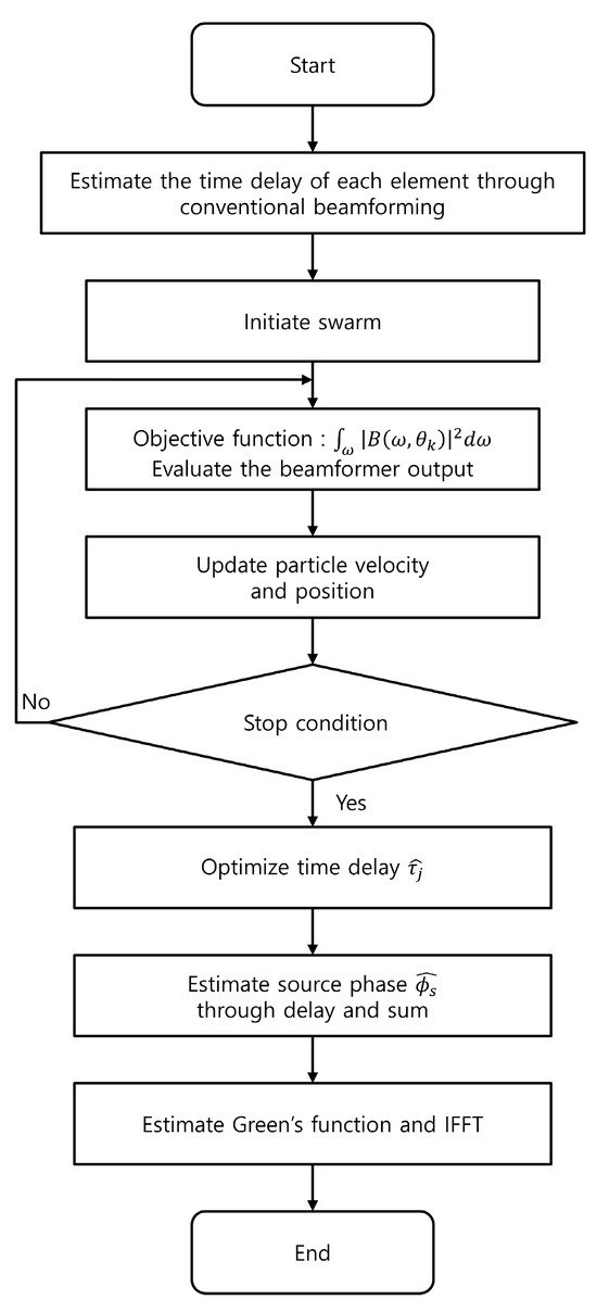
Figure 1.
Flowchart of the RBD-PSO algorithm for searching the optimal time delays for each hydrophone.
3. Experimental Description
Acoustic data collected from the SAVEX15 experiment, which was conducted approximately 100 km south of Jeju Island, Korea, were widely used in previous RBD-related research and were utilized in this study. The water depth at the experiment site was approximately 100 m, and two VLAs, each consisted of 16 elements, were deployed to span half of the water column from 25 to 81 m. Figure 2 illustrates the experimental layout for the segment of the experiment in which the acoustic data analyzed in this study were collected. At 04:11 UTC on 26 May, the R/V Onnuri approached one of the two moored VLAs to a distance of approximately 220 m and then moved away to a distance of approximately 3800 m by 05:01 UTC. During this movement, the R/V Onnuri simultaneously towed two acoustic sources, the ITC-2040X and ITC-1001, which emitted acoustic waves at frequencies of 3–10 kHz and 12–26 kHz, respectively, at a depth of approximately 50 m, while maintaining a nearly constant speed of approximately 1.5 m/s. Continuous wave and LFM signals with varying pulse lengths and bandwidths were transmitted by omnidirectional transducers. To evaluate the proposed method across both high- and low-frequency bands, the high-frequency LFM signals (12–26 kHz), transmitted every 4 min with a 60 ms duration, were analyzed, along with the ship noise data (200–2700 Hz), which represented a lower-frequency band than the towed source.
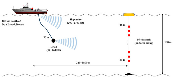
Figure 2.
Experimental layout of acoustic measurements.
Green’s functions were extracted from the LFM signal and ship noise data using 0.12 s and 1 s time windows, respectively. For the ship noise, where the source waveform was unknown, the CIRs were estimated using RBD with both conventional beamforming and the RBD-PSO method proposed in this study. The differences in the CIRs, normalized by the intensity for each array element, were then compared at various distances, with examples provided at approximately 240 m and 900 m. Similarly, for the LFM signal, where the source waveform was known, the CIRs were estimated at multiple distances, with examples presented for 255 m and 1280 m using both methods. The estimated CIRs were then used to reconstruct the source waveform through inverse processing, and cross-correlation coefficients were calculated to quantitatively assess the similarity between the reconstructed and known source waveforms. Furthermore, the effectiveness of the proposed method at improving the arrival time delay estimation was validated by comparing the optimal time delays derived from the PSO with those obtained through matched filtering (MF) at two distances.
4. Results and Discussion
4.1. CIR Estimation in the Low-Frequency Band Using Ship-Radiated Noise
The CIRs were estimated from 1 s recordings of ship noise collected at two distances: approximately 240 m (26 May, 04:12 UTC) and 900 m (26 May, 04:24 UTC), using the ship noise as a low-frequency source. Figure 3a,b present the CIRs, which were normalized for each array element and estimated using RBD and RBD-PSO (denoted as and , respectively) for the 240 m measurements. The arrival paths are clearly illustrated by highlighting a 40 ms segment of the 1 s signal in the figures. A single arrival path was estimated from an element positioned near the sea surface, as the source was located near the surface. When the ship was modeled as a point source positioned at a depth of 2 m, simulated eigenrays obtained using ray-theory-based acoustic propagation modeling [29] for each source–receiver pair confirmed that the direct path and the sea-surface-reflected path arrived at closely adjacent times, which prevented their resolution as separate arrival paths (Figure A2). The exhibited lower noise levels, particularly near the array ends, and displayed arrival paths with shorter durations and sharper peaks compared with , except for certain elements near the center of the array. To quantify the noise reduction in compared with , was defined, which represents the time-averaged difference between the and for each array element as follows:
where is the number of samples in the time series. The metric normalizes the CIRs for each element and then calculates their difference, minimizing the strong sound pressure level variations between the arrival paths and isolating the noise difference. Figure 3c,d depict the element-wise differences, , and the corresponding . The CIR estimation results demonstrate an improvement in most elements, except for the four near the center of the receiving array, with a depth-averaged of 1.9 dB, as indicated by the blue dashed line in Figure 3d.
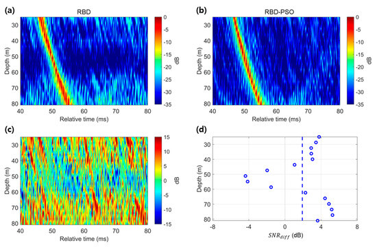
Figure 3.
Normalized intensities for each element representing the CIRs estimated by (a) RBD and (b) RBD-PSO using ship noise (200–2700 Hz) at a range of approximately 240 m. (c) Difference (). (d) for each element (blue circles), with the blue dashed line indicating the depth-averaged of 1.9 dB.
Figure 4 presents and , their difference (), and at a distance of 900 m. Three distinct arrival paths were identified (Figure 4a,b). In contrast to the results at 240 m, where a single arrival path was estimated, at 900 m, the first arrival path was observed from the element positioned closest to the seabed. Eigenray analysis (Figure A2) confirmed that the first arrival path, which appeared as a single path, resulted from the near-simultaneous arrival of the bottom-reflected path (B-path) and the surface–bottom-reflected path (SB-path), which arrived within approximately 0.4 ms of each other at the first element from the sea surface. As the distance increased from 240 m to 900 m, the predicted arrival time difference between the direct and surface-reflected paths decreased from 0.2 ms to 0.001 ms, and thus, became sufficiently small to cause superposition. This superposition led to destructive interference, which prevented these paths from being observed. This prediction was consistent with the CIRs estimated using both RBD and RBD-PSO. In the estimated CIRs, the second arrival path appeared as a single arrival with the strongest intensity, which resulted from the consecutive arrivals of the bottom–surface-reflected path (BS-path) and the surface–bottom–surface-reflected path (SBS-path). The third estimated arrival path was identified as two closely spaced subsequent paths. Each arrival path was found to form a pair, where the second arrival path exhibited the highest intensity due to the coherent summation of the paired paths (Figure A2e). Figure 4c,d show the results obtained using the same method as in Figure 3 to evaluate the performance improvement of the proposed method at 900 m. In Figure 4c, which depicts , the arrival paths in the CIRs were significantly reduced. However, no reduction in the noise level was observed, regardless of the receiver depth. Figure 4d depicts the time-averaged across all 16 elements, which yielded a depth-averaged value of 0.3 dB. Consequently, no significant improvement in the CIR performance was observed at this distance.
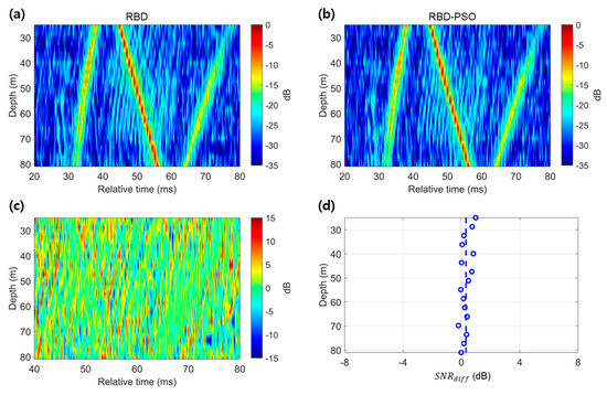
Figure 4.
Normalized intensities for each element representing the CIRs estimated by (a) RBD and (b) RBD-PSO using ship noise (200–2700 Hz) at a range of approximately 900 m. (c) Difference (). (d) for each element (blue circles), with the blue dashed line indicating the depth-averaged of 0.3 dB.
The performance of the CIR estimation in the low-frequency band improved significantly at shorter ranges compared with longer ranges. Figure 5 depicts the relative time delays of each element estimated using conventional beamforming and PSO, along with the differences between the relative time delays obtained from these two methods at approximately 240 m and 900 m. As shown on the left side of Figure 5a, the time delay interval ( between adjacent elements, which was estimated using conventional beamforming, remained constant, as it was determined by the element spacing and the speed of sound in water. In contrast, the intervals estimated using PSO were not constant. On the right side of Figure 5a, the differences in time delays between the two methods for each element exhibited a curved shape, indicating the extent to which the PSO corrected the time delays estimated by conventional beamforming. This discrepancy arose from errors in the conventional beamformer, which assumed a linear relationship based on the speed of sound in water and element spacing but did not account for the spherical wavefront at close range. However, at longer ranges, the relative time delays estimated using both methods became more similar, as the plane-wave approximation held under far-field conditions.
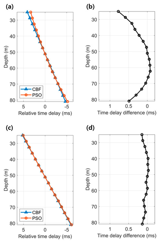
Figure 5.
(a) Relative time delays, referenced to the 8th receiver and estimated using conventional beamforming and PSO at a distance of approximately 240 m, and (b) the corresponding time delay differences for each element. (c,d) show the relative time delays and differences at approximately 900 m, respectively.
The depth-averaged was calculated as a function of distance from 240 m to 3800 m (Figure 6). It decreased rapidly as the distance increased to approximately 400 m. Beyond this distance, it remained mostly below 0.5 dB, indicating no significant performance improvement.
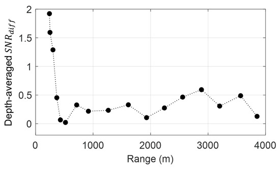
Figure 6.
Depth-averaged as a function of distance.
4.2. Source Waveform Reconstruction Using the CIRs Estimated from LFM Signals in the High-Frequency Band
In the high-frequency band, an LFM signal emitted from a towed source at a depth of 50 m was analyzed at two distances: 255 m (26 May, 04:13 UTC) and 1280 m (26 May, 04:29 UTC). The source waveform was reconstructed through deconvolution of the received signal using the estimated CIRs. Cross-correlation coefficients with the known source waveform were calculated in the same manner in [22]. Since a higher cross-correlation coefficient indicates a greater accuracy in CIR estimation, this metric was used to evaluate the performance improvements. Figure 7 presents the estimated CIRs using RBD and RBD-PSO, along with the short-time Fourier transforms (STFTs) of the reconstructed source waveform at close range. The CIRs estimated using RBD-PSO exhibited arrival paths with shorter durations, sharper peaks, and a higher SNR compared with those obtained using RBD (direct path: ~50 ms; surface-reflected path: ~60–75 ms). The second row of Figure 7 presents the STFTs of the reconstructed source waveform, where the RBD-PSO method demonstrated a higher SNR and a smoother upsweep frequency pattern compared with the RBD estimation. Furthermore, the cross-correlation coefficient with the original source waveform increased significantly from 0.29 to 0.79.
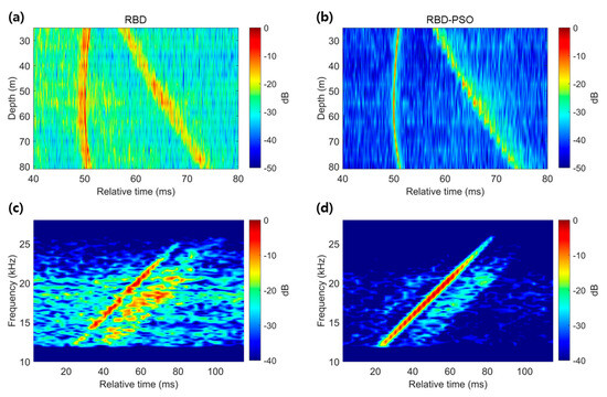
Figure 7.
Normalized intensities of the CIRs estimated by (a) RBD and (b) RBD-PSO at a distance of approximately 255 m between R/V Onnuri and the VLA, with an LFM signal (12–26 kHz). The second row shows the STFTs of the reconstructed source waveform using (c) RBD and (d) RBD-PSO.
The CIRs estimated using RBD and RBD-PSO at a range of 1280 m are shown in Figure 8a and Figure 8b, respectively. The results indicate that multiple paths arrived simultaneously due to refraction effects as the distance increased (Figure A3a). Similar to the findings at shorter ranges, the arrival paths estimated using RBD-PSO exhibited more impulsive features and a higher SNR. This observation was further supported by an increase in the cross-correlation coefficient from 0.43 with RBD to 0.84 with RBD-PSO. Additionally, an eigenray tracing analysis was conducted by simulating a source depth of 50 m, which differed from the low-frequency band case. This analysis confirmed that surface-reflected or bottom-reflected paths arrived earlier than the direct path (Figure A3).
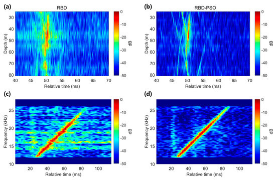
Figure 8.
Normalized intensities of the CIRs estimated by (a) RBD and (b) RBD-PSO at a distance of approximately 1280 m between the R/V Onnuri and the VLA with an LFM signal (12–26 kHz). The second row shows the STFTs of the reconstructed source waveform using (c) RBD and (d) RBD-PSO.
Figure 8c,d present the STFTs of the reconstructed source waveform. The cross-correlation coefficient increased from 0.43 to 0.84, demonstrating a performance improvement comparable with that observed at shorter distances. This result contrasts with the ship noise results in the low-frequency band, where performance improvements were only observed at a short range but not at a long range.
Figure 9 depicts the relative time delays for each element estimated using conventional beamforming, MF, and PSO at two distances. In Figure 9a, conventional beamforming assumed a plane wave, which resulted in relative time delays that appeared as a straight line. In contrast, the relative time delays estimated using PSO closely matched those obtained through MF, which could be considered the ground truth. Additionally, the acoustic wavefronts exhibited a curved shape caused by the direct path that arrived slightly later at both ends of the array due to spherical spreading. The relative time delays at a range of 1280 m are shown in Figure 9b. For the ship noise case, the relative time delays estimated using conventional beamforming and PSO were nearly identical, as the acoustic wavefront conformed to the plane-wave assumption at longer distances. However, for the LFM signal case, the relative time delays differed from those estimated using conventional beamforming, even at a sufficiently large distance, where the wavefront was expected to approximate a plane wave. This discrepancy arose because the ship-radiated noise was generated near the sea surface, whereas the LFM signal was emitted closer to the sound channel axis, where acoustic wave refraction was more pronounced (Figure A3). Furthermore, RBD-PSO accurately estimated the time delay corresponding to the direction of strong arrival paths, which are identified refracted direct paths (Figure A3d). Additionally, the relative time delays estimated using PSO were nearly identical to the MF results, even at long distances.
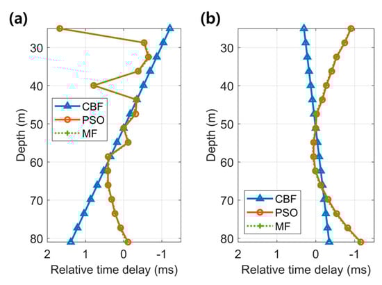
Figure 9.
Relative time delays, referenced to the 8th receiver and estimated using conventional beamforming, PSO, and matched filtering at distances of approximately (a) 255 m and (b) 1280 m.
For the high-frequency band, the performance improvement was evaluated at varying distances. Figure 10 presents the cross-correlation coefficients between the original source waveform and the source waveforms reconstructed using RBD and RBD-PSO as the distance increased from approximately 255 m to 3800 m. At all distances, RBD-PSO achieved higher cross-correlation coefficients in the source waveform reconstruction compared with RBD. Although the magnitude of improvement varied with distance, the CIRs were estimated more accurately in the high-frequency band, which led to a clear performance enhancement.
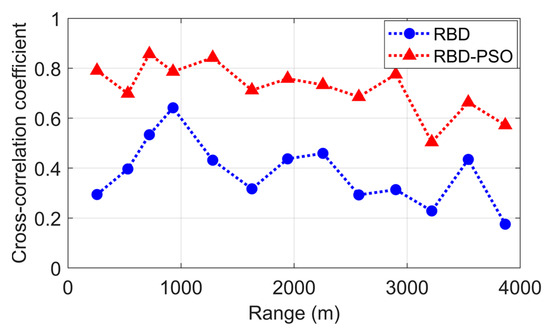
Figure 10.
Cross-correlation coefficients between the original and reconstructed source waveforms from RBD and RBD-PSO as a function of the range.
5. Conclusions
This paper proposes a method to enhance the CIR estimation performance of the RBD technique, which is widely used in underwater acoustics. In the RBD process, CIRs are estimated by determining the phase of the source waveform through the summation of received signals, each adjusted with time delays corresponding to the direction of the maximum beamformer output. The proposed RBD-PSO method improved the source phase estimation by integrating the PSO algorithm into the RBD framework to obtain more precise time delays. This method was applied to subsets of acoustic data collected by a VLA during the SAVEX15 experiment, which included ship-radiated noise for the low-frequency band and LFM signals for the high-frequency band, at both short and long distances. Its performance was evaluated by comparing the results with those obtained using the conventional approach. The findings demonstrate more compact arrival paths with reduced time spread and a higher SNR, except in the low-frequency band at long distances. Notably, in the high-frequency band, where the wavelengths are relatively short, the proposed method achieved significant performance improvements regardless of distance. Furthermore, the proposed method successfully estimated the time delays in both relatively simple environments, where individual propagation paths were clearly distinguishable, and more complex scenarios that involved multiple simultaneous arrival paths (Figure A3).
A key advantage of the proposed method is its ability to correct phase distortions caused by signal interference, which become more pronounced at higher frequencies due to shorter wavelengths. While near-field beamforming techniques can also address time alignment issues when far-field conditions are not met at short distances, our approach offers an effective alternative by incorporating an optimization algorithm into the time alignment process for array-received signals. In contrast to conventional methods that assume a plane wave, the proposed approach enhances CIR estimation by compensating for unexpected or nonlinear influences, such as refraction due to variations in the sound speed structure and array tilt caused by ocean currents. This refinement will enhance its applicability in underwater acoustic research, where precise CIR estimation is essential. Nevertheless, further research is needed to evaluate its performance under more challenging conditions, such as a lower SNR condition caused by unexpected signals or increased source–receiver distances, which were not explicitly examined in this study.
Future research will focus on applying the proposed method to enhance the reliability of geoacoustic inversion through bottom reflection loss estimation. Furthermore, the method has the potential to be extended to broader applications that involve high-frequency signals with unknown source waveforms, such as marine mammal localization [30] and underwater acoustic communications [31], thereby expanding its impact across various underwater acoustic studies.
Author Contributions
Conceptualization, W.Y. and D.-G.H.; methodology, W.Y. and D.-G.H.; formal analysis, W.Y.; investigation, W.Y.; data curation, W.Y.; writing—original draft preparation, W.Y.; writing—review and editing, D.-G.H.; visualization, W.Y.; supervision, D.-G.H. All authors have read and agreed to the published version of the manuscript.
Funding
This work was supported by Korea Research Institute for defense Technology planning and advancement (KRIT)-Grant funded by Defense Acquisition Program Administration (DAPA), South Korea (KRIT-CT-23-026, Integrated Underwater Surveillance Research Center for Adapting Future Technologies, 2023–2029).
Data Availability Statement
The original contributions presented in this study are included in this article; further inquiries can be directed to the corresponding author.
Acknowledgments
The authors thank J. W. Choi for his comments on this research.
Conflicts of Interest
The authors declare no conflicts of interest.
Appendix A
To validate the selected PSO parameters (inertia weight, cognitive and social coefficients), analyses were conducted for low-frequency (240 m and 900 m) and high-frequency (255 m and 1280 m) scenarios. In these analyses, 50 particles with 500 iterations were used for the low-frequency band, while 150 particles with 1000 iterations were used for the high-frequency band—ten times fewer than in Section 4, where a larger number of particles was employed to enhance the accuracy of the time delay estimation. The objective function was calculated and averaged over ten trials for each parameter combination by varying three PSO parameters: inertia weight from 0.25 to 2, and cognitive and social coefficients from 0.25 to 3, all in increments of 0.25. The results of the parameter analysis are presented in Figure A1.
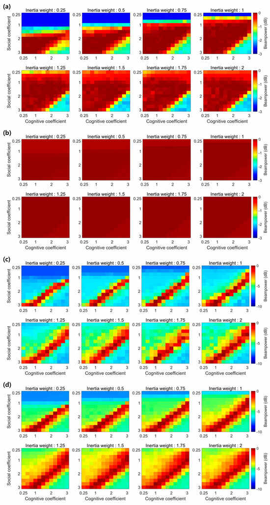
Figure A1.
Parameter analysis results for different frequency bands and distances: low-frequency band at distances of approximately (a) 240 m and (b) 900 m; high-frequency band at distances of approximately (c) 255 m and (d) 1280 m.
Appendix B
The destructive interference between the direct path and the surface-reflected path in the low-frequency band as the distance increased was investigated by simulating the CIRs using eigenray tracing for the source-to-VLA distances of 240 m and 900 m (Figure A2). The sound speed profiles were calculated using the temperature and depth data from thermistor strings installed on the VLA during the experiment. Notably, although the experiment was conducted in a shallow-water environment, the sound speed profile exhibited a minimum at mid-depth—a characteristic more commonly observed in deep-water environments [6,32].
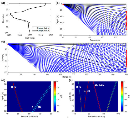
Figure A2.
(a) Sound speed profiles. Simulated CIRs between the source and the VLA at distances of (b) 240 m and (c) 900 m in the low-frequency band, where black and blue lines represent direct paths and multipath trajectories, respectively. Simulated CIRs between the source and the VLA at (d) 240 m and (e) 900 m in the low-frequency band.
In the high-frequency band, where the source depth was 50 m, the sound speed profile also exhibited a mid-depth minimum, which created an environment where surface- or bottom-reflected paths arrived earlier than the direct path. Ray trajectories and the arrival times of multipaths were simulated for a source-to-VLA distance of 1280 m (Figure A3). Figure A3d shows the simulated CIRs, which confirmed that the time delays estimated using PSO and MF in Figure 9b were caused by refraction. Due to this refraction, the direct path arrived at various angles, and multipaths, including the bottom- and surface-reflected paths, were received simultaneously, which resulted in a complex arrival pattern. The red-dotted lines with circles represent the strongest arrival path for each element. The simulation results indicate that the time delays estimated by PSO and MF corresponded to the direct path, which arrived later than the surface- or bottom-reflected paths but exhibited a stronger amplitude. Specifically, discrepancies were observed at two depths, which corresponded to the second and fifth elements from the sea surface showing discrepancies compared with the simulation results (see the white dashed boxes in Figure A3d). These differences can be attributed to the following: At the second element, two direct paths were observed in the measured data, whereas only one was predicted in the simulation. At the fifth element, the amplitude at the overlapping arrival time of the bottom-reflected and direct paths (~48.5 ms) was larger in the measured data, whereas in the simulation, the strongest amplitude was associated with another direct path that arrived at approximately 50 ms.
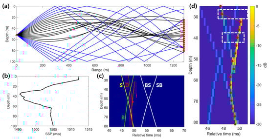
Figure A3.
(a) Ray trajectories (black lines: direct paths; blue lines: multipath trajectories) and (b) corresponding sound speed profile during the experiment. In (a), the black lines represent the direct paths, and the blue lines indicate multipath components. (c) Simulated arrival times of the multipath components and (d) CIRs between the source and the VLA at a distance of 1280 m in the high-frequency band. The red dotted lines with circular markers represent the relative times of the strongest received paths for each receiver (white dashed boxes indicate depths where the CIRs estimated using RBD-PSO differed from the simulation).
References
- Sabra, K.G.; Song, H.-C.; Dowling, D.R. Ray-based blind deconvolution in ocean sound channels. J. Acoust. Soc. Am. 2010, 127, EL42–EL47. [Google Scholar] [CrossRef]
- Zhang, X.; Durofchalk, N.C.; Niu, H.; Wu, L.; Zhang, R.; Sabra, K.G. Geoacoustic inversion using ray-based blind deconvolution of shipping sources. J. Acoust. Soc. Am. 2020, 147, 285–299. [Google Scholar] [CrossRef] [PubMed]
- Kim, D.; Park, H.; Kim, J.; Hahn, J.Y. Application of ray-based blind deconvolution to long-range acoustic communication in deep water. J. Acoust. Soc. Korea 2022, 41, 242–253. [Google Scholar]
- Lee, S.; Makris, N.C. The array invariant. J. Acoust. Soc. Am. 2006, 119, 336–351. [Google Scholar] [CrossRef] [PubMed]
- Byun, G.; Kim, J.; Cho, C.; Song, H.; Byun, S.-H. Array invariant-based ranging of a source of opportunity. J. Acoust. Soc. Am. 2017, 142, EL286–EL291. [Google Scholar] [CrossRef]
- Song, H.-C.; Cho, C.; Byun, G.; Kim, J.S. Cascade of blind deconvolution and array invariant for robust source-range estimation. J. Acoust. Soc. Am. 2017, 141, 3270–3273. [Google Scholar] [PubMed]
- Byun, G.; Song, H.; Kim, J.; Park, J. Real-time tracking of a surface ship using a bottom-mounted horizontal array. J. Acoust. Soc. Am. 2018, 144, 2375–2382. [Google Scholar] [CrossRef]
- Durofchalk, N.C.; Sabra, K.G. Analysis of the ray-based blind deconvolution algorithm for shipping sources. J. Acoust. Soc. Am. 2020, 147, 1927–1938. [Google Scholar]
- Touret, R.X.; Durofchalk, N.; Sabra, K.G. Quantifying the influence of source motion on the ray-based blind deconvolution algorithm. JASA Express Lett. 2024, 4, 116002. [Google Scholar] [CrossRef]
- Byun, S.-H.; Byun, G.; Sabra, K.G. Ray-based blind deconvolution of shipping sources using multiple beams separated by alternating projection. J. Acoust. Soc. Am. 2018, 144, 3525–3532. [Google Scholar]
- Kim, D.; Kim, D.; Byun, G.; Kim, J.; Song, H. Improvement of a Green’s Function Estimation for a Moving Source Using the Waveguide Invariant Theory. Sensors 2024, 24, 5782. [Google Scholar] [CrossRef]
- Xu, Z.; Li, H.; Yang, K.; Li, P. A deep-water ray-based blind deconvolution for a near-surface source with a bottom-moored short-aperture vertical array. JASA Express Lett. 2022, 2, 026001. [Google Scholar] [CrossRef] [PubMed]
- Zhang, X.; Yang, J.; Sabra, K. Ray-based blind deconvolution of shipping sources using single-snapshot adaptive beamforming. J. Acoust. Soc. Am. 2020, 147, EL106–EL112. [Google Scholar]
- Abadi, S.H.; Rouseff, D.; Dowling, D.R. Blind deconvolution for robust signal estimation and approximate source localization. J. Acoust. Soc. Am. 2012, 131, 2599–2610. [Google Scholar] [PubMed]
- Song, H.; Cho, C. Array invariant-based source localization in shallow water using a sparse vertical array. J. Acoust. Soc. Am. 2017, 141, 183–188. [Google Scholar]
- Yoon, S.; Yang, H.; Seong, W. Ray-based blind deconvolution with maximum kurtosis phase correction. J. Acoust. Soc. Am. 2022, 151, 4237–4251. [Google Scholar] [CrossRef]
- Kennedy, J.; Eberhart, R. Particle swarm optimization. In Proceedings of the Proceedings of ICNN’95-International Conference on Neural Networks, Perth, WA, Australia, 27 November–1 December 1995; pp. 1942–1948. [Google Scholar]
- AlRashidi, M.R.; El-Hawary, M.E. A survey of particle swarm optimization applications in electric power systems. IEEE Trans. Evol. Comput. 2008, 13, 913–918. [Google Scholar]
- Liu, F.; Zhou, Z. An improved QPSO algorithm and its application in the high-dimensional complex problems. Chemom. Intell. Lab. Syst. 2014, 132, 82–90. [Google Scholar] [CrossRef]
- Sen, M.K.; Stoffa, P.L. Global Optimization Methods in Geophysical Inversion; Cambridge University Press: Cambridge, UK, 2013. [Google Scholar]
- Byun, G.; Cho, C.; Song, H.; Kim, J.; Byun, S.-H. Array invariant-based calibration of array tilt using a source of opportunity. J. Acoust. Soc. Am. 2018, 143, 1318–1325. [Google Scholar] [CrossRef]
- Byun, S.-H.; Verlinden, C.; Sabra, K.G. Blind deconvolution of shipping sources in an ocean waveguide. J. Acoust. Soc. Am. 2017, 141, 797–807. [Google Scholar]
- Poli, R.; Kennedy, J.; Blackwell, T. Particle swarm optimization: An overview. Swarm Intell. 2007, 1, 33–57. [Google Scholar]
- Gutiérrez, A.; Lanza, M.; Barriuso, I.; Valle, L.; Domingo, M.; Perez, J.; Basterrechea, J. Comparison of different PSO initialization techniques for high dimensional search space problems: A test with FSS and antenna arrays. In Proceedings of the Proceedings of the 5th European Conference on Antennas and Propagation (EUCAP), Rome, Italy, 11–15 April 2011; pp. 965–969. [Google Scholar]
- Helwig, S.; Wanka, R. Particle swarm optimization in high-dimensional bounded search spaces. In Proceedings of the 2007 IEEE Swarm Intelligence Symposium, Honolulu, HI, USA, 1–5 April 2007; pp. 198–205. [Google Scholar]
- Yahya, A.A.; Osman, A.; El-Bashir, M.S. Rocchio algorithm-based particle initialization mechanism for effective PSO classification of high dimensional data. Swarm Evol. Comput. 2017, 34, 18–32. [Google Scholar]
- Xinchao, Z. A perturbed particle swarm algorithm for numerical optimization. Appl. Soft Comput. 2010, 10, 119–124. [Google Scholar]
- Wang, D.; Tan, D.; Liu, L. Particle swarm optimization algorithm: An overview. Soft Comput. 2018, 22, 387–408. [Google Scholar]
- Porter, M.B.; Bucker, H.P. Gaussian beam tracing for computing ocean acoustic fields. J. Acoust. Soc. Am. 1987, 82, 1349–1359. [Google Scholar] [CrossRef]
- Gong, Z.; Ratilal, P.; Makris, N.C. Simultaneous localization of multiple broadband non-impulsive acoustic sources in an ocean waveguide using the array invariant. J. Acoust. Soc. Am. 2015, 138, 2649–2667. [Google Scholar]
- Oh, S.H.; Byun, G.H.; Kim, J. Performance improvement of underwater acoustic communication using ray-based blind deconvolution in passive time reversal mirror. J. Acoust. Soc. Korea 2016, 35, 375–382. [Google Scholar]
- Jensen, F.B.; Kuperman, W.A.; Porter, M.B.; Schmidt, H.; Tolstoy, A. Computational Ocean Acoustics; Springer: Berlin/Heidelberg, Germany, 2011; Volume 2011. [Google Scholar]
Disclaimer/Publisher’s Note: The statements, opinions and data contained in all publications are solely those of the individual author(s) and contributor(s) and not of MDPI and/or the editor(s). MDPI and/or the editor(s) disclaim responsibility for any injury to people or property resulting from any ideas, methods, instructions or products referred to in the content. |
© 2025 by the authors. Licensee MDPI, Basel, Switzerland. This article is an open access article distributed under the terms and conditions of the Creative Commons Attribution (CC BY) license (https://creativecommons.org/licenses/by/4.0/).