Research on the Visual SLAM Algorithm for Unmanned Surface Vehicles in Nearshore Dynamic Scenarios

Abstract

To address the challenges of visual SLAM algorithms in unmanned surface vehicles (USVs) during nearshore navigation or docking, where dynamic feature points degrade localization accuracy and dynamic objects impede static dense mapping, this study proposes an improved visual SLAM algorithm that removes dynamic feature points. Building upon the ORB-SLAM3 framework, the improved SLAM algorithm integrates a shore segmentation module and a dynamic region elimination module, while enabling static dense point cloud mapping. The system first implements shore segmentation based on Otsu’s method to generate masks covering water and sky regions, ensuring the SLAM system avoids extracting interfering feature points from these areas. Secondly, the deep learning network YOLOv8n-seg is employed to detect priori dynamic objects, with the motion consistency check method to identify non-priori dynamic feature points, collectively removing dynamic feature points. Additionally, the ELAS algorithm computes disparity maps, integrating depth information and dynamic object information to construct a static dense map. Experimental results demonstrate that, compared to the original ORB-SLAM3, the improved SLAM algorithm achieves superior localization accuracy in dynamic nearshore environments, significantly reduces the impact of dynamic objects on pose estimation, and successfully constructs ghosting-free static dense point cloud maps.

1. Introduction

With the advancement of technology, unmanned systems have gained widespread applications across industries. Autonomous vehicles and drones have penetrated civilian domains, while unmanned surface vehicles (USVs) [1] are rapidly evolving, gradually replacing human-operated tasks in aquatic environments. For USVs to perform surface operations, continuous positional information acquisition is essential. In recent years, visual simultaneous localization and mapping (SLAM) technology [2,3,4,5,6] has seen rapid development due to the affordability of cameras and the rich information provided by visual data and has found applications in autonomous driving [7], drones, and other fields. This progress also offers insights into USV autonomous localization. While numerous studies have integrated visual systems with sensors such as GNSS and IMU [8], challenges persist: GNSS signals may degrade in occluded environments, and IMUs are prone to drift or failure during prolonged operation or under insufficient motion excitation. Notably, vision-dominant SLAM systems face significant interference from nearshore dynamic objects, water reflections, and surface fluctuations when USVs navigate or dock nearshore. Thus, eliminating the impact of nearshore dynamic interference on visual SLAM systems is critical.

Currently, many visual SLAM algorithms for dynamic scenes improve robustness by treating dynamic feature points as outliers and removing them. Early studies mainly focused on detecting dynamic features using traditional methods, such as inter-frame errors, camera geometric constraints, or optical flow. In 2013, Tan et al. [9] used the reprojection error between two frames to determine whether a feature point was in motion. However, this method struggled to distinguish dynamic points effectively when dynamic objects moved slowly. In 2017, Sun et al. [10] proposed applying the homography matrix estimated by RANSAC to the pixels of the previous frame to detect dynamic objects using the inter-frame difference method. They further enhanced dynamic object detection with a particle filter. However, the RANSAC algorithm relies on a large amount of static data to determine whether a point is dynamic. When dynamic objects occupy a large area, static points may instead be misclassified as outliers and removed. In 2019, Wang et al. [11] proposed a method that filters feature point correspondences between adjacent frames using epipolar geometry and clusters depth map data to segment dynamic objects. However, this approach exhibited substantial errors when handling highly dynamic objects. In 2019, Fan et al. [12] decomposed camera motion into translational and rotational components, leveraging these geometric constraints to localize dynamic regions. They further integrated multi-frame information to reconstruct occluded backgrounds and suppress dynamic interference. In 2019, Cheng et al. [13] proposed a method based on optical flow values for distinguishing dynamic points in real time and integrated it into a feature-based monocular SLAM system. However, the system suffered from tracking loss when dynamic objects occupied a significant portion of the image. In 2020, Dai et al. [14] used the Delaunay triangulation method to construct a sparse graph, where points with unchanged relative positions were considered correlated, establishing the correlation between map points. They then calculated the areas of all correlated subgraphs, with the largest one representing the static region. In 2023, Ali et al. [15] applied the motion information of optical flow in a visual-inertial SLAM system to remove dynamic feature points. They also used the scene information carried by the optical flow method to construct a dense map. In 2024, Zhang et al. [16] introduced a mask prediction mechanism and a dual-polar optical flow tracking method that fused ORB features with optical flow, thereby selectively allocating computational resources to enhance real-time performance. With the advancement of deep learning [17] technology, many object detection and semantic segmentation algorithms have been introduced into visual SLAM systems. In 2018, Zhong et al. [18] proposed the Detect-SLAM algorithm, which detects prior dynamic objects in the environment using a single shot multibox detector (SSD) [19] to remove feature points on dynamic objects. To improve real-time performance, the algorithm performs detection only on keyframes and propagates motion probability using feature matching and matched point expansion. In 2018, Wang et al. [20] integrated YOLO object detection into the SLAM system, but the algorithm was designed only for indoor environments. Relying solely on traditional methods, such as inter-frame error, camera geometric constraints, or optical flow, often suffers from high computational complexity, susceptibility to lighting variations, and suboptimal feature point removal. On the other hand, approaches that solely integrate deep learning are limited to detecting only prior dynamic objects. Therefore, some researchers have proposed combining both methods to eliminate dynamic feature points jointly. In 2018, Yu et al. [21] introduced DS-SLAM, a dynamic SLAM framework integrating epipolar geometry with SegNet [22] semantic segmentation network to eliminate dynamic feature points and improve localization accuracy. Concurrently, Bescos et al. [23] proposed Dyna-SLAM, which leverages the Mask R-CNN [24] instance segmentation network to generate dynamic object masks. This approach combines multi-view geometry to remove dynamic feature points and performs background inpainting by fusing prior and current frames. However, the Mask R-CNN network imposes high computational requirements and leads to prolonged system processing time. In 2020, Han et al. [25] employed the PSPNet network [26] for semantic segmentation to generate dynamic object masks, combined with the motion consistency check to eliminate dynamic regions by filtering unstable feature points. In 2021, Liu et al. [27] proposed RDS-SLAM (real-time dynamic SLAM), a framework built upon ORB-SLAM3 that leverages semantic information to suppress the interference of dynamic objects. By parallelizing semantic and optimization threads with the tracking thread, RDS-SLAM eliminates latency caused by waiting for semantic processing. In 2023, Yu et al. [28] proposed the YG-SLAM algorithm, which constructs a YOLOv5 object detection thread outside the tracking thread. This approach combines the LK optical flow method to determine the instantaneous motion speed of feature points, aiding in the removal of potential dynamic feature points.

Existing dynamic SLAM algorithms primarily focus on eliminating dynamic objects on land, while dynamic feature points caused by water surface fluctuations, reflections, and clouds are rarely specifically addressed. However, these feature points often interfere with USV localization. Moreover, mainstream feature-based SLAM algorithms such as ORB-SLAM3, as well as dynamic SLAM algorithms based on ORB-SLAM3, predominantly utilize sparse feature points for mapping, making it difficult to achieve high-precision scene reconstruction. To better address the issue of visual SLAM being disrupted by nearshore dynamic feature points, which affect localization accuracy, and the limitation of ORB-SLAM3 in achieving dense mapping, this paper proposes a dynamic SLAM algorithm based on the ORB-SLAM3 framework. This SLAM algorithm first performs shore segmentation on images, then integrates the YOLOv8n-seg network into the tracking thread to detect priori dynamic objects, combined with the motion consistency check to identify non-priori dynamic feature points, further suppressing dynamic interference, thereby improving the localization accuracy. At the same time, the algorithm achieves dense mapping for nearshore environments.

The innovations are summarized as follows:

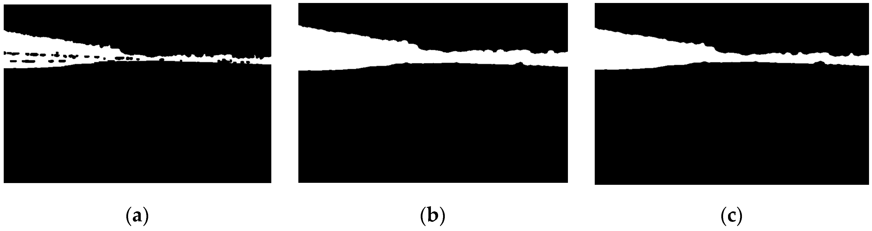
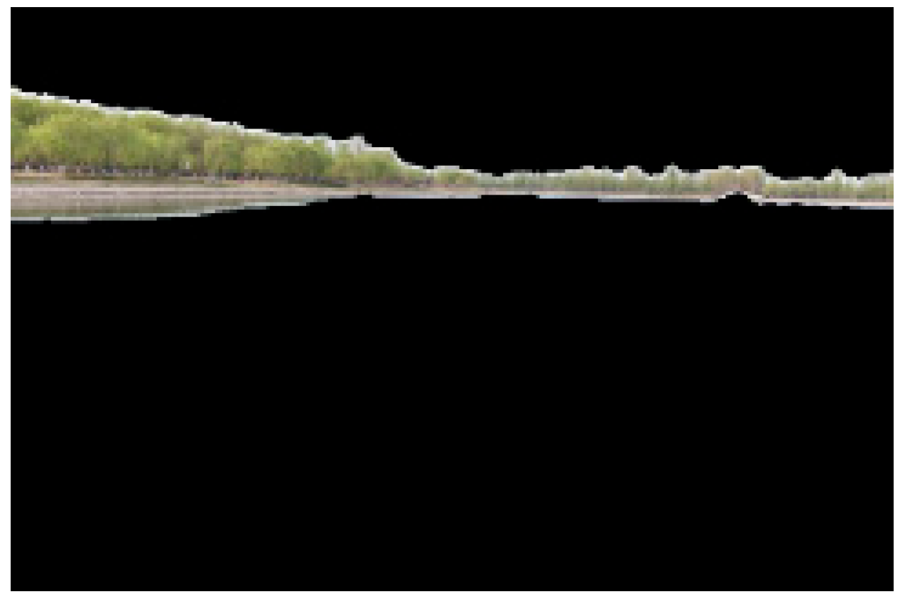
• To address the challenge of extracting invalid feature points from water and sky regions during nearshore navigation, a shore segmentation based on Otsu’s method is proposed. The input image is converted to the HSV color space, where the H channel is isolated. Otsu’s method is then applied for shore segmentation, followed by morphological operations to denoise and refine boundaries, ultimately generating masks for water and sky regions.
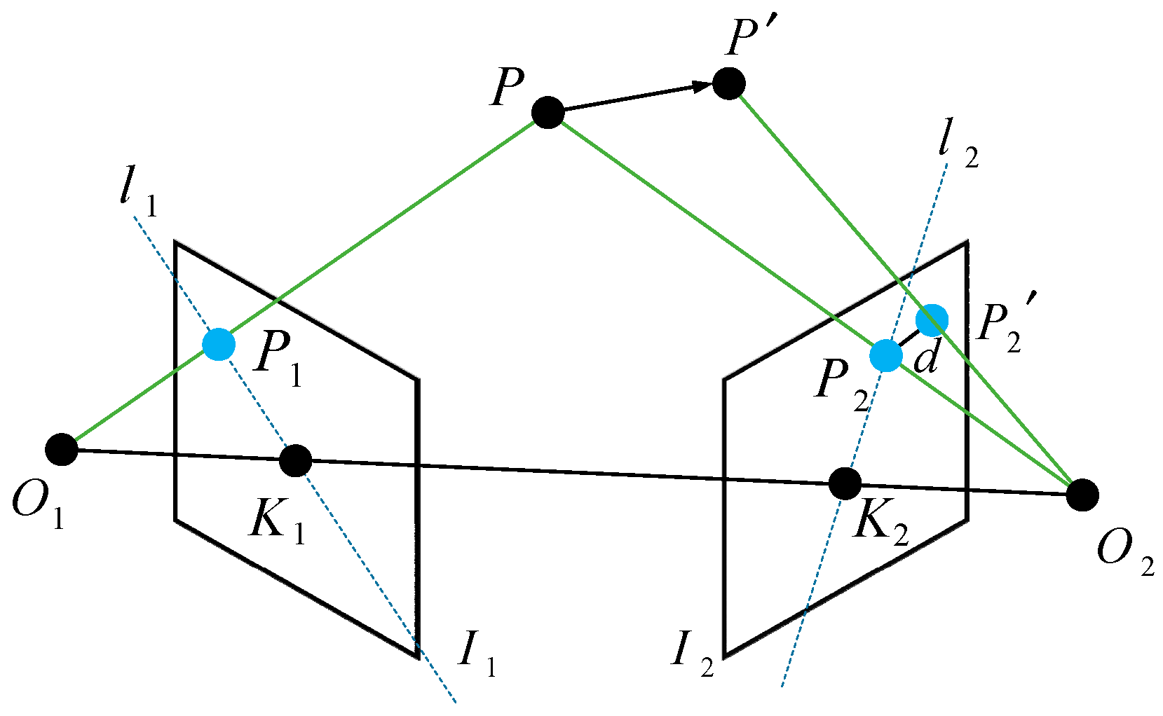
• YOLOv8 instance segmentation is embedded into the visual SLAM system to detect priori dynamic objects, producing dynamic object masks. Feature points within these masked regions are identified and excluded. For non-priori dynamic feature points, the motion consistency check method is applied to validate the static/dynamic status of remaining feature points, further eliminating potential dynamic interference and enhancing localization accuracy in dynamic environments.
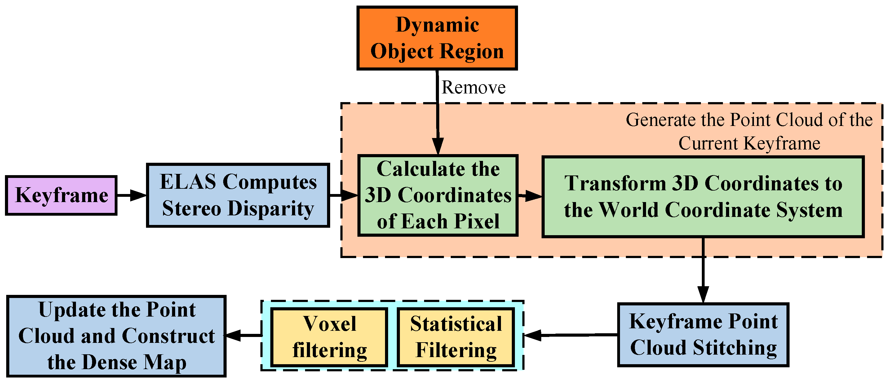
• A dense mapping thread is added, leveraging the efficient large-scale stereo matching (ELAS) [29] algorithm to compute depth information and construct 3D point clouds. By removing dynamic objects from images, ghosting artifacts in point cloud data caused by moving objects are eliminated, enabling the construction of static dense maps.

The structure of this paper is as follows: Section 2 systematically introduces the proposed methods, including shore segmentation, dynamic object detection and removal, and dense mapping techniques. Section 3 demonstrates the effectiveness of shore segmentation, non-prior dynamic feature point removal, localization trajectory comparison, and dense mapping through real-world experiments. It also compares the localization accuracy with other dynamic SLAM algorithms using the TUM dynamic dataset. Section 4 provides the conclusion of this paper.

2. System Introduction

2.1. System Framework

To address the localization degradation caused by nearshore dynamic feature points in existing visual SLAM algorithms for USV, this study proposes an improved dynamic visual SLAM algorithm based on the ORB-SLAM3 framework, with the system architecture illustrated in Figure 1. The improved SLAM algorithm achieves shore segmentation, dynamic object detection and removal, and static dense mapping. During the image input stage, a shore segmentation based on Otsu’s method is applied to segment images to generate masks covering water and sky regions, thereby restricting ORB feature extraction exclusively to the shore areas. In the tracking thread, the YOLOv8n-seg network detects and segments priori dynamic objects, removing dynamic feature points within their corresponding masks. For feature points outside these masks, the motion consistency check method is applied to distinguish dynamic feature points. The dense mapping thread receives processed keyframes with dynamic objects removed and combines depth information from ELAS with pose estimation data to construct 3D point clouds. These point clouds undergo filtering to remove noise and outliers and are aligned sequentially to construct a static dense point cloud map.

2.2. Shore Segmentation Based on Otsu’s Method

USVs operate in aquatic environments, where their nearshore perspective typically comprises three regions: water, shore, and sky. Feature point extraction in such environments is inevitably affected by water reflections, water ripples, and clouds in the sky. Excessive invalid feature points from water and sky regions degrade localization accuracy. In response to this challenge, shore segmentation based on Otsu’s method is implemented to isolate shore regions and avoid extracting invalid feature points from water and sky areas.

Otsu’s method determines an optimal threshold to separate a single-channel image into two classes: pixels below the threshold and those above or equal to it. The optimal threshold maximizes the inter-class variance between these two classes.

Images captured by cameras are typically in the RGB color space. However, the red (R), green (G), and blue (B) channels exhibit high linear correlation and strong interdependencies, which makes them suboptimal for threshold-based segmentation tasks. Thus, the images are converted to the HSV color space, and the H channel is isolated for thresholding, as illustrated in Figure 2.

In the H-channel image, sky and water regions are grouped into a single category, while shore regions are distinctly separated. Otsu’s method is applied to the H-channel to generate a binary image of the shore and other areas. The conversion process is as follows [30]:

$${\sigma }^2(t)={\omega }_0(t){({\mu }_T-{\mu }_0(t))}^2+{\omega }_1(t){({\mu }_T-{\mu }_1(t))}^2$$

(1)

Here, $t$ represents the gray threshold (ranging from 0 to L-level grayscale), ${\sigma }^2(t)$ is the inter-class variance, ${\omega }_0(t)$ and ${\omega }_1(t)$ denote the pixel proportions of the foreground and background classes, respectively, ${\mu }_0(t)$ and ${\mu }_1(t)$ are their respective mean gray values, and ${\mu }_T$ is the global mean gray values. The threshold $t$ corresponding to the maximum inter-class variance ${\sigma }^2(t)$ is selected to produce a binary segmentation.

After segmentation, the binary image still contains noise and gaps. To overcome this drawback, the binary image is first inverted, followed by an erosion operation to eliminate noise. A dilation operation is then applied to connect gaps within the shore region. However, dilation may cause the shore contour to expand outward excessively. To mitigate this, a secondary erosion operation is performed, counteracting the over-expansion from the previous step. The results of these three morphological operations and the original image overlaid with the final mask are shown in Figure 3 and Figure 4, respectively.

The shore segmentation based on Otsu’s method can segment the shore area and obtain a mask covering the water and sky regions. By applying this mask during ORB feature point extraction, the system restricts feature point extraction to the shore region.

2.3. Dynamic Object Detection and Removal

2.3.1. Priori Dynamic Object Detection

For the validation of prior dynamic objects, two approaches are considered: detection and segmentation. Compared to detection-based methods, segmentation algorithms can more accurately separate dynamic objects from the surrounding environment, preserving more static feature points. The mainstream segmentation network models include Mask-CNN, SegNet, U-Net, PSPNet, DeepLabV3+, YOLO, etc. Among them, Mask-CNN uses a two-stage processing method, which achieves high segmentation accuracy but has a slower inference speed. PSPNet, DeepLabV3+, U-Net, and SegNet provide only semantic segmentation, unable to separate individual instances, and are more suitable for scene segmentation. In contrast, YOLO offers an end-to-end training and inference process, simplifying the computational procedure and achieving high-speed inference while ensuring high segmentation accuracy, making it suitable for SLAM scenarios that require high real-time performance.

Considering that USVs are embedded devices, this study adopts the YOLOv8n-seg network [31,32,33,34], the most lightweight variant of YOLOv8 instance segmentation, to segment these priori dynamic objects. The network architecture of YOLOv8n-seg is illustrated in Figure 5. The backbone network extracts foundational features, the neck network performs multi-scale feature fusion across hierarchical layers, and the detection head executes object detection and classification. Compared to the YOLOv8 object detection framework, the instance segmentation variant (YOLOv8n-seg) incorporates an additional segmentation branch to generate pixel-level masks for dynamic objects.

The network is trained on the COCO dataset, split into training, testing, and validation sets at a 20:4:1 ratio. After YOLOv8n-seg completes inference on the image, the system first checks whether any detected objects belong to priori dynamic categories. If such objects are present, it iterates through all extracted feature points to determine if they lie within the bounding boxes of these priori dynamic objects. For feature points inside the bounding boxes, the system further verifies whether they reside within the corresponding segmentation masks. Points within the masks are discarded, while others are retained. Figure 6 illustrates the segmentation results in a real-world nearshore scenario: (a) the original image and (b) the output after detection and segmentation. YOLOv8n-seg performs detection and segmentation of both the person and boat in the scene.

While YOLOv8n-seg effectively removes feature points on priori dynamic objects, non-priori dynamic feature points may persist. To address this, the motion consistency check method is applied to the remaining feature points, ensuring comprehensive dynamic feature point elimination.

2.3.2. Non-Priori Dynamic Feature Point Detection

The discrimination of non-priori dynamic object feature points primarily relies on camera motion consistency. After extracting feature points from image frames, the Lucas-Kanade (LK) optical flow method is applied to track these feature points, establishing correspondences between consecutive frames. This tracking enables the recovery of camera motion between adjacent frames. The epipolar geometry is then used to verify if feature points match static geometric relationships from camera motion, separating static and dynamic points.

The LK optical flow algorithm operates under the brightness constancy assumption, treating images as time-varying functions. It computes feature point correspondences between frames using spatial and temporal image gradients. To enhance robustness matches near image boundaries or those exhibiting significant pixel intensity differences within local regions are discarded, retaining only reliable correspondences for calculating the fundamental matrix $F$.

Motion consistency check validates the static/dynamic status of feature points through epipolar geometric constraint. As illustrated in Figure 7, $O_1$ and $O_2$ represent the optical centers of the cameras for frames $I_1$ and $I_2$, respectively, while $P$ denotes a 3D spatial point, with $P_1$ and $P_2$ being its projections onto the image planes $I_1$ and $I_2$. The projection of a dynamic spatial point $P^{\prime }$ onto $I_2$ is denoted as $P_2^{\prime }$. The rays $O_1{P}_1$ and $O_2{P}_2$ intersect at $P$, forming the epipolar plane $P{O}_1{O}_2$ along with the baseline $O_1{O}_2$. This epipolar plane intersects the image planes $I_1$ and $I_2$ along the epipolar lines $l_1$ and $l_2$, while the baseline intersects the image planes at the epipoles $K_1$ and $K_2$.

Using the fundamental matrix $F$ and the spatial correspondence of feature point $P$, the epipolar line corresponding to this point in the $I_2$ plane is computed. Assuming the epipolar line is represented by the equation $Ax+By+C=0$, the equation of the epipolar line in the $I_2$ plane can be formulated as follows:

$$F{P}_1=F\left[\begin{array}{c}{x}_1\\ y_1\\ 1\end{array}\right]=l_2=\left[\begin{array}{c}A\\ B\\ C\end{array}\right]$$

(2)

When the spatial point $P$ is stationary, its projection $P_2$ on the image plane $I_2$ should lie near the epipolar line $l_2$. When the spatial point $P$ is in motion, as the camera moves from frame $I_1$ to $I_2$, the point $P$ relocates to a new position $P^{\prime }$. Consequently, the projection $P_2^{\prime }$ of $P^{\prime }$ onto the image plane $I_2$ deviates from the epipolar line $l_2$. The dynamic status of the feature point can then be determined by calculating the deviation value $d$ between $P_2^{\prime }$ and $l_2$. The deviation $d$ is computed as follows:

$$d={\displaystyle \frac{{P_2}^{T}F{P}_1}{\sqrt{A^2+B^2+C^2}}}$$

(3)

In real-world environments, the projections of stationary feature points onto their corresponding epipolar lines may exhibit non-zero deviations. Therefore, a threshold is set: if the deviation exceeds this threshold, the feature point is classified as dynamic and subsequently removed from the SLAM pipeline.

2.4. Dense Mapping Based on Stereo Matching

The ORB-SLAM3 system constructs only sparse point cloud maps based on feature points, which are insufficient for downstream tasks such as obstacle avoidance and path planning for USVs. To tackle this issue, a dedicated dense mapping thread, independent of the three main SLAM threads, is introduced. New keyframes generated by the local mapping thread are inserted into this thread, enabling real-time dense mapping without compromising system responsiveness. The dense mapping thread computes depth using the ELAS to obtain 3D spatial information, then removes dynamic objects based on their masks to construct static point cloud data. As keyframes are continuously fed into the system, static point clouds from each frame are incrementally integrated. The global point cloud map is updated through loop closure detection and global bundle adjustment (BA), completing the dense mapping process. For the generated massive point cloud data, the voxel grid filter and statistical outlier removal filter are applied for multi-level point cloud filtering to balance map accuracy and computational efficiency. The workflow for dense map construction is illustrated in Figure 8.

The ELAS aims to identify corresponding pixels between left and right images by computing stereo disparity to derive depth values for each pixel. The algorithm begins by selecting stable support points to obtain candidate disparities. The images are first filtered using the Sobel operator to compute feature vectors, which are then used to evaluate the matching cost between pixel pairs in the left and right images. A smaller feature distance indicates a higher similarity between pixels. A pixel is selected as a candidate support point if its minimum and second-minimum feature distances fall within a predefined threshold. Moreover, applying the left–right consistency principle, if the disparity values of matched pixel points in the left and right images are equal, the candidate support point is selected as a support point. A Delaunay triangulation is constructed based on the support points, where each triangle represents a disparity plane. The disparity plane equation, derived from the three vertices of each triangle, serves as the prior probability, while the feature distance quantifies the likelihood probability. These components are integrated into an energy function formulated as follows:

$$E(d)=\beta {‖f^{(l)}-f^{(r)}(d)‖}_l-\log \left[\gamma +\exp (-{\displaystyle \frac{{(d-\mu (S,O^{(l)}))}^2}{2{\sigma }^2}})\right]$$

(4)

The disparity that minimizes the energy function is assigned as the pixel’s disparity. Based on the disparity obtained from ELAS, the depth value of each pixel is calculated. By combining this with the pixel coordinates of the image, the 3D coordinates of the pixel in the point cloud are calculated, and the corresponding color values from the left RGB image are assigned to each point in the cloud.

$$S\left[\begin{array}{c}u\\ v\\ 1\end{array}\right]=K(R{p}_g+t)=K(R\left[\begin{array}{c}{x}_g\\ y_g\\ z_g\end{array}\right]+t),K=\left[\begin{array}{ccc}{f}_x& 0& c_x\\ 0& f_y& c_y\\ 0& 0& 1\end{array}\right]$$

(5)

In the formula, $S$ represents the scaling factor between the depth value and the actual distance, $K$ denotes the camera intrinsic matrix, and the rotation matrix $R$ and translation vector $t$ are derived from the estimated camera pose, with $p_g$ indicating the 3D coordinates in the world coordinate system. The coordinate of point $p_i$ in the point cloud is then computed as follows:

$$p_i=\left[{\begin{array}{ccc}{x}_i& y_i& z\end{array}}_i\right]=\left[\begin{array}{ccc}{\displaystyle \frac{S(u-c_x)}{f_x}}& {\displaystyle \frac{S(v-c_y)}{f_y}}& z_i\end{array}\right]$$

(6)

During point cloud generation, coordinates and pixel information associated with dynamic objects are excluded, and dynamic regions are skipped to prevent ghosting artifacts from contaminating the map. As keyframes are input sequentially, the point clouds generated from each keyframe are converted into the global coordinate system and incrementally aligned, ultimately achieving a dense point cloud map.

To obtain higher-quality maps, a multi-stage filtering pipeline is applied to the point cloud data. Raw point clouds are typically massive and contain outliers, particularly due to overlapping fields of view caused by camera motion, which introduce redundant points and inflate data volume. To enhance computational efficiency and remove outliers, the voxel grid filter, based on spatial grid partitioning, is employed for downsampling, followed by the statistical outlier removal filter that leverages statistical analysis to denoise the point cloud. Finally, the global dense map is refined and updated through loop closure detection and global bundle adjustment (BA).

3. Experiments and Analysis of Results

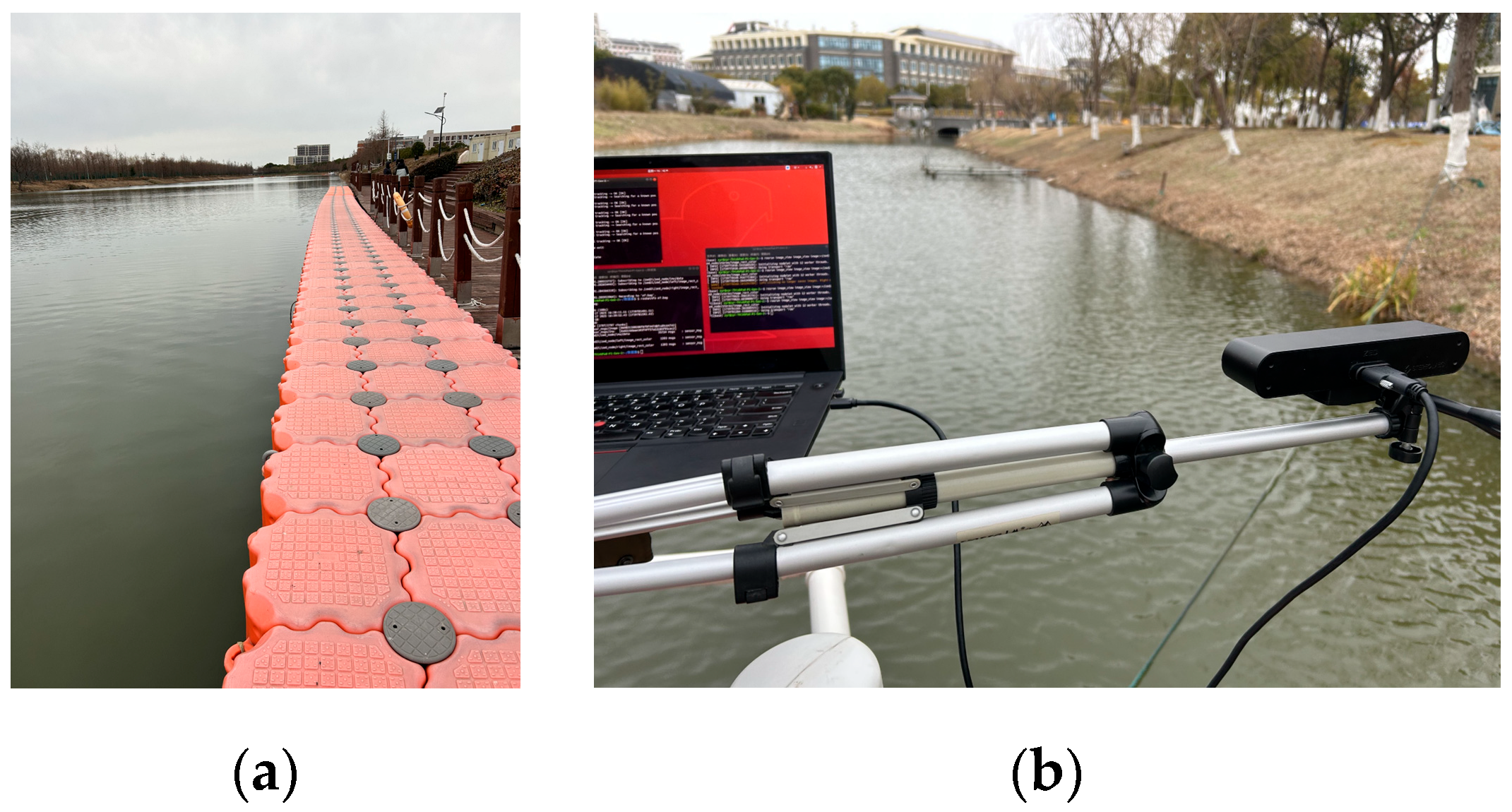
3.1. Experimental Conditions and Datasets

The operating system for the experiments in this paper is Ubuntu 22.04. The hardware used has a memory of 60 GB, and the GPU model is NVIDIA GeForce RTX 4090D (NVIDIA Corporation, Santa Clara, CA, USA) with a video memory of 24 GB. The YOLOv8n-seg network is implemented in Python (Version 3.10), the trained model is converted and then invoked in the SLAM system for inference, and the SLAM system is implemented in C++ (Version 17) and compiled by CMake (Version 3.30.1).

To validate the effectiveness of the proposed algorithm in dynamic nearshore scenarios, three sets of real-world data were collected. Due to equipment limitations, data were acquired using handheld and mounted devices on the bow to simulate USV nearshore navigation or docking scenarios. All data were captured by a ZED2i camera (StereoLabs Corporation, San Francisco, CA, USA), with stereo images and IMU (Inertial Measurement Unit) data functioning as reference trajectories. The stereo camera collected left and right images at 15 Hz, while the IMU recorded inertial data at 350 Hz.

In Scenario 1, the camera was mounted on a tripod placed on a floating platform and manually moved along the platform near the water’s edge. During the experiment, efforts were made to ensure that the camera moved along a straight trajectory to minimize any possible displacement or shaking during the capture process. At the same time, experimental personnel continuously moved in front of the camera to simulate the movement of an unmanned surface vehicle in a nearshore dynamic environment. The experimental scene and equipment setup are shown in Figure 9.

In Scenario 2, the camera was fixed to the bow of a motorized boat, capturing datasets while cruising parallel to the shoreline. In the experiment, the camera is securely fixed at the bow of the boat using a triangular bracket, ensuring its position remains stable and allowing for a precise shooting angle. During the experiment, the boat is manually operated, moving slowly along the lakeshore and gradually approaching the shore. At the same time, pedestrians are active along the shore, and other boats pass by on the water, simulating dynamic factors that mimic the movement of an unmanned surface vehicle in a nearshore dynamic environment. The experimental scene and equipment setup are shown in Figure 10.

In Scenario 1, datasets for both sunny and cloudy days were collected, while in Scenario 2, a dataset for a cloudy day was collected. All the collected data were stored in rosbag files on the computer. To process these data, OpenCV is first used to parse the rosbag files and extract the left and right images, IMU data, and timestamp information. Next, the timestamps are accurately aligned to ensure temporal consistency between data from different sensors. Finally, after these processing steps, the dataset is constructed. The dataset information for the three actual scenes is shown in

Table 1. Dataset information.

Data Name	Number of Left Images (Frames)	Number of Right Images (Frames)	IMU Data (Entries)	Image Size (Pixels)
Scene 1 (cloudy)	741	741	17,665	640 × 360
Scene 1 (sunny)	897	897	21,138	640 × 360
Scene 2	1050	1050	25,064	640 × 360

.

3.2. Experiment on Shore Segmentation Based on Otsu’s Method

To evaluate the effectiveness of the shore segmentation based on Otsu’s method, a comparative experiment was conducted on the images captured in Scenario 1, analyzing ORB feature point extraction before and after applying the segmentation mask. The experimental results are demonstrated in Figure 11: (a) shows the original image, (b) shows the original image with the segmentation mask applied, (c) illustrates the feature point extraction results without the mask, and (d) presents the refined feature point extraction after applying the mask.

As demonstrated by the experimental results, the shore segmentation based on Otsu’s method effectively distinguishes shore regions from water and sky areas in aquatic environment images, successfully generating a mask that covers the water and sky regions. Without mask application, lots of feature points are extracted from the sky and water surface. By contrast, when the mask is applied, the system selectively extracts feature points exclusively within the shore region, thereby minimizing the adverse effects of water ripples, reflections, and sky interference.

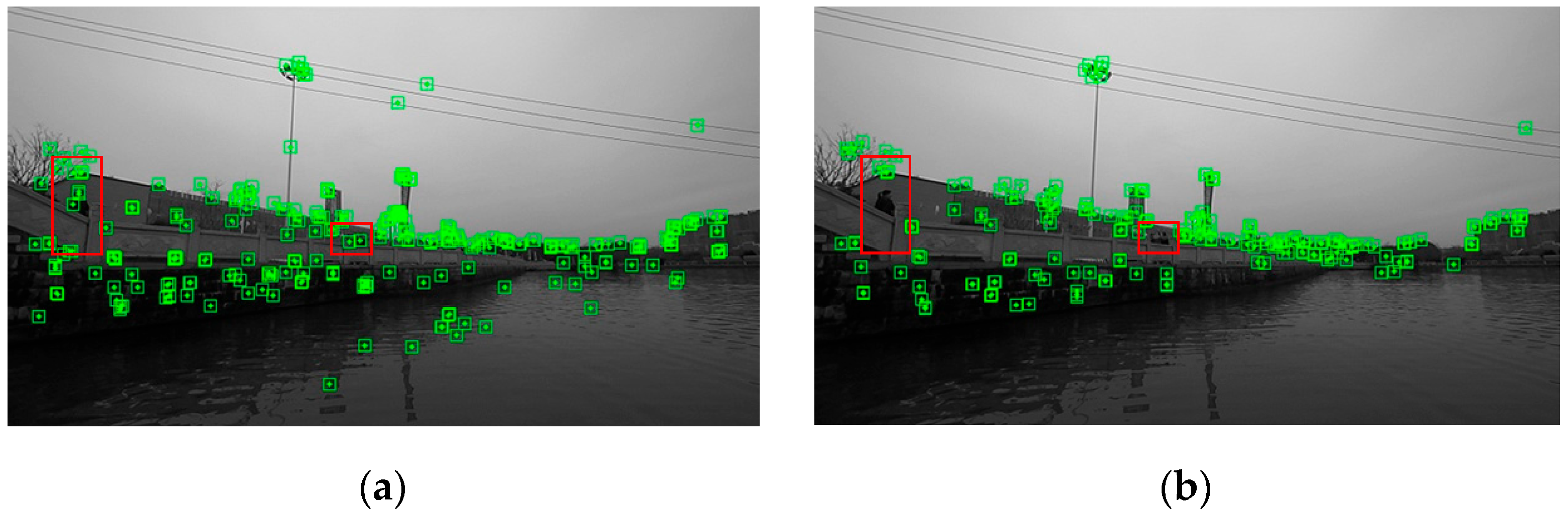
3.3. Non-Priori Dynamic Feature Point Removal Experiment

The results of non-priori dynamic feature points removal are illustrated in Figure 12: (a) shows the result without eliminating non-priori dynamic feature points, while (b) demonstrates the refined results after applying motion consistency check to remove non-priori dynamic feature points. The results reveal that the original ORB-SLAM3 system extracts feature points from a moving hand, and such non-priori dynamic objects adversely affect subsequent pose estimation, leading to degraded localization accuracy. By integrating the motion consistency check, feature points on the moving hand are eliminated, ensuring that only static feature points contribute to downstream computations. This refinement effectively shields the system from the interference of dynamic objects.

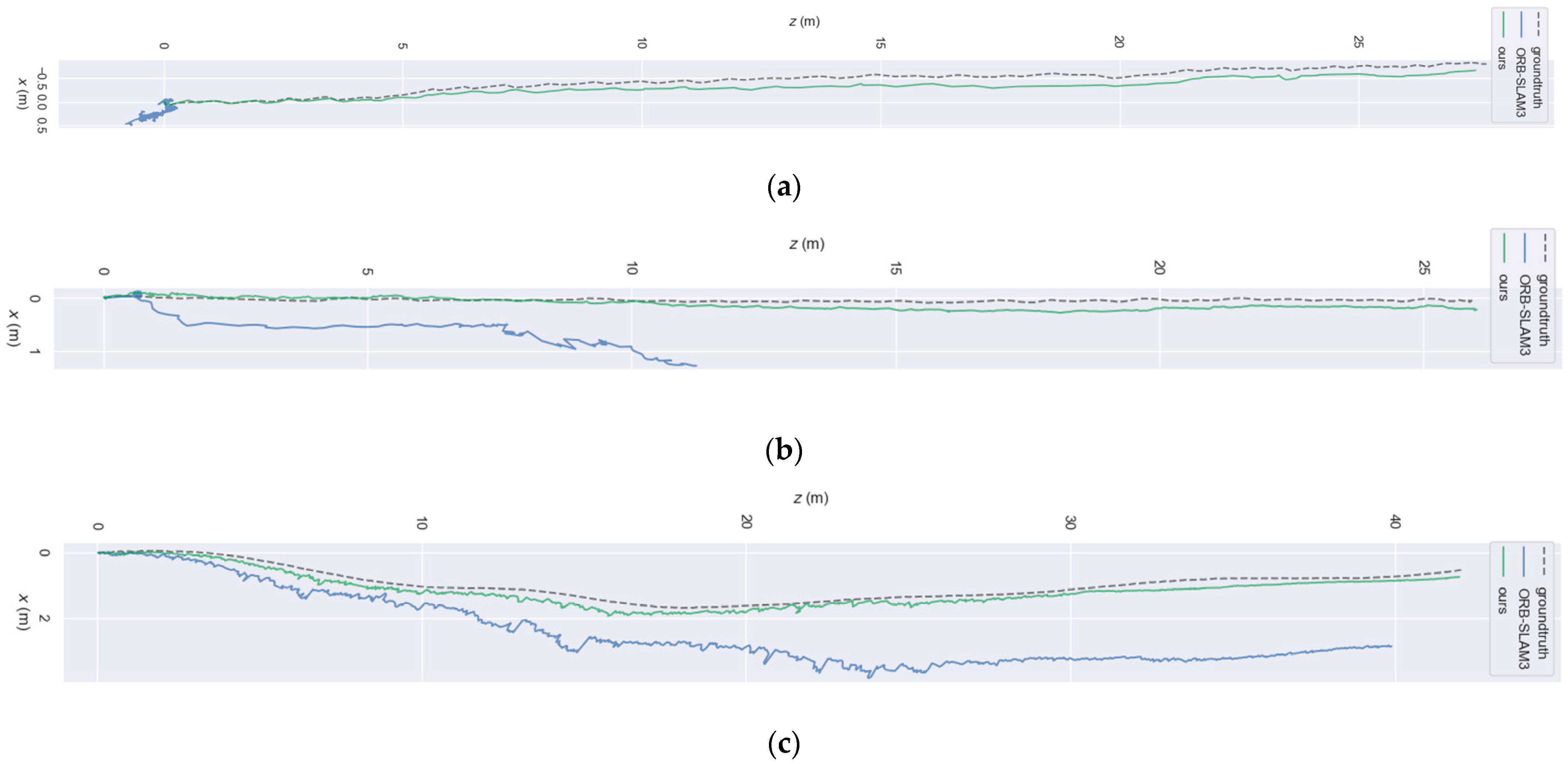
3.4. Visual SLAM Localization Validation

The imaging results and feature point extraction outcomes for Scenarios 1 (sunny and cloudy) and 2 are presented in Figure 13, Figure 14 and Figure 15, respectively. (a) shows the result without removing dynamic objects and water surface feature points, and (b) shows the result after removing dynamic objects and water surface feature points.

In experimental Scenario 1, under sunny conditions, the main factors influencing feature point extraction were the ripples on the water surface and pedestrians walking along the shore, while under cloudy conditions, the water surface reflections and pedestrians walking along the shore affected feature extraction. Additionally, under the backlit conditions of cloudy weather, ORB-SLAM3 was only able to extract the contour points of pedestrians, whereas, in sunny conditions with good lighting, the ORB-SLAM3 algorithm extracted a large number of dynamic feature points from the pedestrians. After integrating YOLOv8n-seg, feature points on pedestrians were effectively eliminated. Furthermore, all feature points caused by water surface fluctuations and reflections were filtered by applying the shore segmentation. In Scenario 2, pedestrians occupied a smaller portion of the frame and were partially occluded by railings. Despite these challenges, the YOLOv8n-seg successfully identified and removed pedestrian-associated feature points, and the shore segmentation filtered out water reflections and ripples, thereby significantly reducing the impact of water disturbances on feature point extraction and localization accuracy.

The trajectory comparisons of the two real-world scenarios are illustrated in Figure 16, where the Z-axis represents the forward direction, and the X-axis represents the lateral deviation. Scenario 1 was characterized by a highly dynamic environment with frequent pedestrian activity along the shoreline. Under sunny conditions with clear lighting, the ORB-SLAM3 algorithm extracted a large number of dynamic feature points from pedestrians. When the walking speed of pedestrians and the camera were the same, the estimated trajectory remained almost stationary. Under cloudy, backlit conditions, the influence of dynamic feature points was smaller, so the trajectory did not stay stationary. However, a significant deviation still occurred, ultimately leading to a noticeable difference between the estimated trajectory and the true trajectory. In contrast, the improved SLAM algorithm maintained stable localization by removing dynamic objects, reducing their impact on feature point extraction, and achieving trajectory estimates closely aligned with the ground truth. In Scenario 2, where dynamic objects were relatively sparse, the original ORB-SLAM3 algorithm maintained continuous localization. However, occasional dynamic objects (e.g., pedestrians, vessels) and persistent water surface fluctuations in the image sequence induced trajectory drift. The improved SLAM algorithm successfully eliminated dynamic objects, water reflections, and surface ripples, resulting in a generated trajectory that closely aligns with the ground truth.

3.5. Comparison with Other Dynamic SLAM Algorithms

In order to further validate the localization performance of the proposed algorithm, the TUM open-source dynamic dataset was selected for comparison between the proposed algorithm and existing dynamic SLAM algorithms. The root mean square error (RMSE) of the absolute trajectory error (ATE) was used as the localization accuracy evaluation metric. The walking_xyz, walking_rpy, walking_halfsphere, and walking_static sequences of the dataset were executed, and the results are shown in

Table 2. Comparison of the RMSE of the absolute trajectory error.

Data Sequence	Dyna-SLAM [23] (Mask-CNN)	DS-SLAM [21] (SegNet)	RDS-SLAM [27] (Mask-CNN)	Detect-SLAM [18] (SSD)	Ours (YOLOv8)
w_xyz	0.015	0.025	0.057	0.024	0.014
w_rpy	0.035	0.444	0.160	0.030	0.038
w_halfsphere	0.025	0.030	0.026	0.051	0.020
w_static	0.006	0.008	0.021	—	0.007

.

The results show that, in high-dynamic environments, the proposed algorithm achieves localization accuracy comparable to Dyna-SLAM, with errors within the centimeter range, while significantly outperforming DS-SLAM, RDS-SLAM, and Detect-SLAM. In terms of real-time performance, the average frame tracking time of Dyna-SLAM exceeds 300 ms, whereas the proposed algorithm maintains a stable frame tracking time of under 100 ms. Therefore, compared to Dyna-SLAM, the proposed algorithm not only ensures similar localization accuracy but also improves real-time performance, making it more suitable for unmanned surface vehicle nearshore visual SLAM tasks, which require higher computational efficiency.

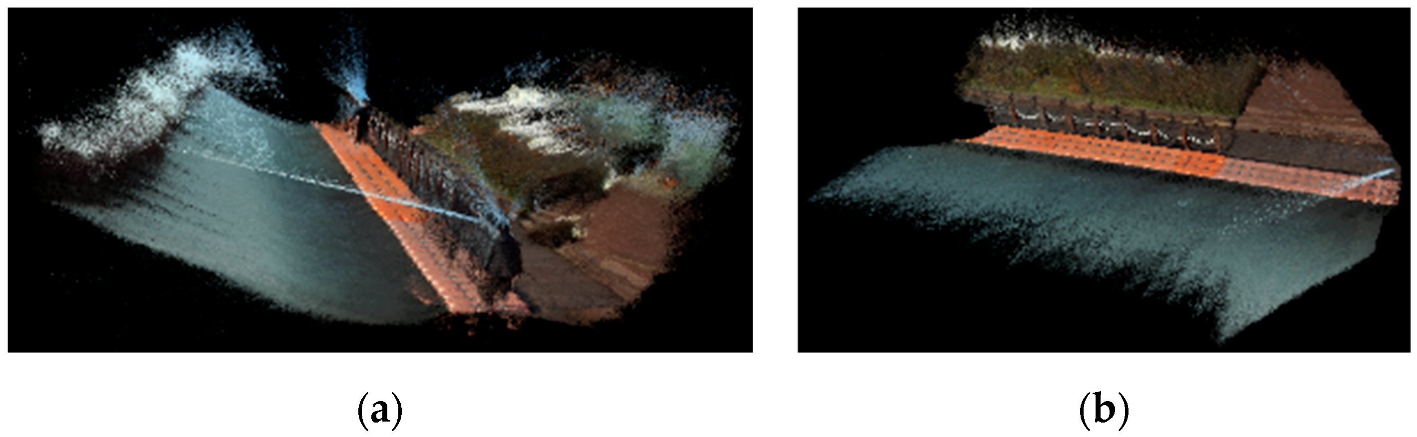
3.6. Validation of Static Dense Mapping

Scenario 1 was selected for dense map construction to verify the effectiveness of dense mapping. The resulting dense map is shown in Figure 17. As shown in Figure 14, in the validation of Scenario 1, the activity of pedestrians introduced significant ghosting artifacts into the dense map when dynamic objects were not removed. However, after applying dynamic object removal, these ghosting artifacts were effectively eliminated, constructing a ghosting-free dense map. Since dense mapping relies on keyframe data, and the motion speed between the camera and pedestrians was comparable in Scenario 1, previously occluded areas were restored as pedestrians moved to new positions. This allowed the system to construct dense point clouds for the newly exposed regions and fill gaps, ensuring the continuity of the dense map after the dynamic objects were removed.

4. Conclusions

This paper focuses on the issue of inaccurate localization in unmanned surface vehicles during nearshore navigation, caused by dynamic feature points that affect visual SLAM algorithms. An improved dynamic SLAM algorithm based on stereo vision is proposed. First, the shore segmentation based on Otsu’s method effectively extracts shore regions, thereby eliminating interference feature points from water and sky areas and enhancing the robustness of the SLAM system in aquatic environments. Secondly, YOLOv8-seg effectively identifies and removes priori dynamic objects (e.g., pedestrians, vessels) in images. For non-priori dynamic objects, the improved SLAM algorithm integrates the motion consistency check to detect and eliminate such dynamic feature points. This dual strategy, combining semantic segmentation with geometric validation, significantly enhances the localization accuracy of visual SLAM in highly dynamic nearshore environments. Finally, the newly added dense mapping thread successfully eliminates ghosting artifacts caused by dynamic objects and successfully constructs a static dense map.

The algorithm proposed in this paper demonstrates good robustness when the USV faces high-dynamic nearshore environments. It optimizes the performance of visual SLAM in such environments, enhancing the applicability of visual SLAM and providing a reliable optimization solution for visual navigation in unmanned surface vehicles. The algorithm is particularly suitable for scenarios where GNSS signals are unstable (e.g., under bridges or in complex coastal environments), IMU acceleration is insufficient, or sensor resources are limited (e.g., lightweight USVs). It ensures short-term autonomous localization of the USV in dynamic nearshore environments, even when sensor data is unreliable. However, as the algorithm still relies on visual information, it may be affected by extreme lighting changes or adverse weather conditions. Future research will further explore multi-sensor fusion to improve stability in extreme weather or turbulent environments.

References

1. Ghazali, M.H.M.; Satar, M.H.A.; Rahiman, W. Unmanned Surface Vehicles: From a Hull Design Perspective. Ocean Eng. 2024, 312, 118977. [Google Scholar] [CrossRef]
2. Mur-Artal, R.; Montiel, J.M.M.; Tardos, J.D. ORB-SLAM: A Versatile and Accurate Monocular SLAM System. IEEE Trans. Robot. 2015, 31, 1147–1163. [Google Scholar] [CrossRef]
3. Mur-Artal, R.; Tardos, J.D. ORB-SLAM2: An Open-Source SLAM System for Monocular, Stereo and RGB-D Cameras. IEEE Trans. Robot. 2017, 33, 1255–1262. [Google Scholar] [CrossRef]
4. Campos, C.; Elvira, R.; Rodríguez, J.J.G.; Montiel, J.M.M.; Tardós, J.D. ORB-SLAM3: An Accurate Open-Source Library for Visual, Visual-Inertial and Multi-Map SLAM. IEEE Trans. Robot. 2021, 37, 1874–1890. [Google Scholar] [CrossRef]
5. Qin, T.; Li, P.; Shen, S. VINS-Mono: A Robust and Versatile Monocular Visual-Inertial State Estimator. IEEE Trans. Robot. 2018, 34, 1004–1020. [Google Scholar] [CrossRef]
6. Qin, T.; Cao, S.; Pan, J.; Shen, S. A General Optimization-Based Framework for Global Pose Estimation with Multiple Sensors. arXiv 2019, arXiv:1901.03642. [Google Scholar]
7. Cheng, J.; Zhang, L.; Chen, Q.; Hu, X.; Cai, J. A Review of Visual SLAM Methods for Autonomous Driving Vehicles. Eng. Appl. Artif. Intell. 2022, 114, 104992. [Google Scholar]
8. Wu, H.; Chen, Y.; Yang, Q.; Yan, B.; Yang, X. A Review of Underwater Robot Localization in Confined Spaces. J. Mar. Sci. Eng. 2024, 12, 428. [Google Scholar] [CrossRef]
9. Tan, W.; Liu, H.; Dong, Z.; Zhang, G.; Bao, H. Robust Monocular SLAM in Dynamic Environments. In Proceedings of the 2013 IEEE International Symposium on Mixed and Augmented Reality (ISMAR), Adelaide, Australia, 1–4 October 2013; pp. 209–218. [Google Scholar]
10. Sun, Y.; Liu, M.; Meng, M.Q.-H. Improving RGB-D SLAM in Dynamic Environments: A motion Removal Approach. Robot. Auton. Syst. 2017, 89, 110–122. [Google Scholar]
11. Wang, R.; Wan, W.; Wang, Y.; Di, K. A New RGB-D SLAM Method with Moving Object Detection for Dynamic Indoor Scenes. Remote Sens. 2019, 11, 1143. [Google Scholar] [CrossRef]
12. Fan, Y.; Han, H.; Tang, Y.; Zhi, T. Dynamic Objects Elimination in SLAM Based on Image Fusion. Pattern Recognit. Lett. 2019, 127, 191–201. [Google Scholar] [CrossRef]
13. Cheng, J.; Sun, Y.; Meng, M.Q.-H. Improving Monocular Visual SLAM in Dynamic Environments: An Optical-Flow-Based Approach. Adv. Robot. 2019, 33, 576–589. [Google Scholar] [CrossRef]
14. Dai, W.; Zhang, Y.; Li, P.; Fang, Z.; Scherer, S. Rgb-d Slam in Dynamic Environments Using Point Correlations. IEEE Trans. Pattern Anal. Mach. Intell. 2020, 44, 373–389. [Google Scholar] [CrossRef] [PubMed]
15. Samadzadeh, A.; Nickabadi, A. SRVIO: Super Robust Visual Inertial Odometry for Dynamic Environments and Challenging Loop-Closure Conditions. IEEE Trans. Robot. 2022, 39, 2878–2891. [Google Scholar] [CrossRef]
16. Zhang, Y.; Bujanca, M.; Luján, M. NGD-SLAM: Towards Real-Time SLAM for Dynamic Environments without GPU. arXiv 2024, arXiv:2405.07392. [Google Scholar]
17. Cai, D.; Li, R.; Hu, Z.; Lu, J.; Li, S.; Zhao, Y. A Comprehensive Overview of Core Modules in Visual SLAM Framework. Neurocoputing 2024, 590, 127760. [Google Scholar] [CrossRef]
18. Zhong, F.; Wang, S.; Zhang, Z.; Chen, C.; Wang, Y. Detect-SLAM: Making Object Detection and SLAM Mutually Beneficial. In Proceedings of the 2018 IEEE Winter Conference on Applications of Computer Vision (WACV), Lake Tahoe, NV, USA, 12–15 March 2018; pp. 1001–1010. [Google Scholar]
19. Liu, W.; Anguelov, D.; Erhan, D.; Szegedy, C.; Reed, S.; Fu, C.-Y.; Berg, A.C. Ssd: Single Shot Multibox Detector. In Proceedings of the Computer Vision–ECCV 2016: 14th European Conference, Amsterdam, The Netherlands, 11–14 October 2016; Proceedings, Part I 14. Springer: Cham, Switzerland, 2016; Volume 9905, pp. 21–37. [Google Scholar]
20. Wang, R.; Wang, Y.; Wan, W.; Di, K. A Point-Line Feature Based Visual SLAM Method in Dynamic Indoor Scene. In Proceedings of the 2018 Ubiquitous Positioning, Indoor Navigation and Location-Based Services (UPINLBS), Wuhan, China, 22–23 March 2018; pp. 1–6. [Google Scholar]
21. Yu, C.; Liu, Z.; Liu, X.-J.; Xie, F.; Yang, Y.; Wei, Q.; Fei, Q. DS-SLAM: A Semantic Visual SLAM towards Dynamic Environments. In Proceedings of the 2018 IEEE/RSJ International Conference on Intelligent Robots and Systems (IROS), Madrid, Spain, 1–5 October 2018; pp. 1168–1174. [Google Scholar]
22. Badrinarayanan, V.; Kendall, A.; Cipolla, R. SegNet: A Deep Convolutional Encoder-Decoder Architecture for Image Segmentation. IEEE Trans. Pattern Anal. Mach. Intell. 2017, 39, 2481–2495. [Google Scholar] [CrossRef]
23. Bescos, B.; Fácil, J.M.; Civera, J.; Neira, J. DynaSLAM: Tracking, Mapping and Inpainting in Dynamic Scenes. IEEE Robot. Autom. Lett. 2018, 3, 4076–4083. [Google Scholar] [CrossRef]
24. He, K.; Gkioxari, G.; Dollár, P.; Girshick, R. Mask R-CNN. In Proceedings of the IEEE International Conference on Computer Vision, Venice, Italy, 22–29 October 2018. [Google Scholar]
25. Han, S.; Xi, Z. Dynamic Scene Semantics SLAM Based on Semantic Segmentation. IEEE Access 2020, 8, 43563–43570. [Google Scholar] [CrossRef]
26. Zhao, H.; Shi, J.; Qi, X.; Wang, X.; Jia, J. Pyramid Scene Parsing Network. In Proceedings of the 2017 IEEE Conference on Computer Vision and Pattern Recognition, Honolulu, HI, USA, 21–26 July 2017. [Google Scholar]
27. Liu, Y.; Miura, J. RDS-SLAM: Real-Time Dynamic SLAM Using Semantic Segmentation Methods. IEEE Access 2021, 9, 23772–23785. [Google Scholar] [CrossRef]
28. Yu, Y.; Zhu, K.; Yu, W. YG-SLAM: GPU-Accelerated RGBD-SLAM Using YOLOv5 in a Dynamic Environment. Electronics 2023, 12, 4377. [Google Scholar] [CrossRef]
29. Geiger, A.; Roser, M.; Urtasun, R. Efficient Large-Scale Stereo Matching. In Proceedings of the Asian Conference on Computer Vision, Queenstown, New Zealand, 8–12 November 2010; Springer: Berlin/Heidelberg, Germany, 2010; pp. 25–38. [Google Scholar]
30. Otsu, N. A Threshold Selection Method from Gray-Level Histograms. Automatica 1975, 11, 23–27. [Google Scholar]
31. Diwan, T.; Anirudh, G.; Tembhurne, J.V. Object Detection Using YOLO: Challenges, Architectural Successors, Datasets and Applications. Multimed. Tools Appl. 2023, 82, 9243–9275. [Google Scholar] [CrossRef] [PubMed]
32. Terven, J.; Córdova-Esparza, D.-M.; Romero-González, J.-A. A Comprehensive Review of YOLO Architectures in Computer Vision: From YOLOv1 to YOLOv8 and YOLO-NAS. Mach. Learn. Knowl. Extr. 2023, 5, 1680–1716. [Google Scholar] [CrossRef]
33. Vijayakumar, A.; Vairavasundaram, S. YOLO-Based Object Detection Models: A Review and its Applications. Multimed. Tools Appl. 2024, 83, 83535–83574. [Google Scholar] [CrossRef]
34. Hussain, M. YOLOv1 to v8: Unveiling Each Variant–A Comprehensive Review of YOLO. IEEE Access 2024, 12, 42816–42833. [Google Scholar] [CrossRef]
Figure 1. Overall system framework.
Jmse 13 00679 g001
Figure 2. H component transformation comparison. (a) Original image; (b) H-channel image.
Jmse 13 00679 g002
Figure 3. Results after three morphological operations. (a) Primary erosion; (b) dilation; (c) secondary erosion.
Jmse 13 00679 g003
Figure 4. Mask overlay on the original image.
Jmse 13 00679 g004
Figure 5. YOLOv8n-seg network architecture.
Jmse 13 00679 g005
Figure 6. Segmentation results. (a) Original image; (b) detection and segmentation results.
Jmse 13 00679 g006
Figure 7. Geometric constraint scene graph.
Jmse 13 00679 g007
Figure 8. Dense point cloud construction process.
Jmse 13 00679 g008
Figure 9. Experimental scene and equipment of Scene 1. (a) The experimental scene; (b) experimental equipment.
Jmse 13 00679 g009
Figure 10. Experimental scene and equipment of Scene 2. (a) The experimental scene; (b) experimental equipment.
Jmse 13 00679 g010
Figure 11. Segmentation results. (a) Original image; (b) mask overlay on the original image; (c) ORB feature points extraction without mask application; (d) ORB feature points extraction with mask application.
Jmse 13 00679 g011
Figure 12. Comparison of feature point removal effectiveness. (a) The non-prior dynamic objects not removed; (b) remove non-prior dynamic objects.
Jmse 13 00679 g012
Figure 13. Feature extraction results in Scenario 1 under sunny conditions. (a) Dynamic feature points not removed; (b) remove dynamic feature points.
Jmse 13 00679 g013
Figure 14. Feature extraction results in Scenario 1 under cloudy conditions. (a) Dynamic feature points not removed; (b) remove dynamic feature points.
Jmse 13 00679 g014
Figure 15. Feature extraction results in Scenario 2. (a) Dynamic feature points not removed; (b) remove dynamic feature points.
Jmse 13 00679 g015
Figure 16. Comparison of trajectories in real-world scenarios. (a) Comparison of trajectories in real-world scenario 1 (sunny); (b) comparison of trajectories in real-world scenario 1 (cloudy); (c) comparison of trajectories in real-world scenario 2.
Jmse 13 00679 g016
Figure 17. Static dense map of Scenario 1. (a) Dense point clouds without dynamic object removal; (b) dense point clouds with dynamic object removal.
Jmse 13 00679 g017