Article

Multi-Channel Underwater Acoustic Signal Analysis Using Improved Multivariate Multiscale Sample Entropy

by
Jing Zhou
1,2,
Yaan Li
1,* and
Mingzhou Wang
2
1
School of Marine Science and Technology, Northwestern Polytechnical University, Xi’an 710072, China
2
Xi’an Precision Machinery Research Institute, National Key Laboratory of Underwater Information and Control, Xi’an 710077, China
*
Author to whom correspondence should be addressed.
J. Mar. Sci. Eng. 2025, 13(4), 675; https://doi.org/10.3390/jmse13040675
Submission received: 19 February 2025 / Revised: 23 March 2025 / Accepted: 25 March 2025 / Published: 27 March 2025
(This article belongs to the Special Issue Navigation and Detection Fusion for Autonomous Underwater Vehicles)

Abstract

:
Underwater acoustic signals typically exhibit non-Gaussian, non-stationary, and nonlinear characteristics. When processing real-world underwater acoustic signals, traditional multivariate entropy algorithms often struggle to simultaneously ensure stability and extract cross-channel information. To address these issues, the improved multivariate multiscale sample entropy (IMMSE) algorithm is proposed, which extracts the complexity of multi-channel data, enabling a more comprehensive and stable representation of the dynamic characteristics of complex nonlinear systems. This paper explores the optimal parameter selection range for the IMMSE algorithm and compares its sensitivity to noise and computational efficiency with traditional multivariate entropy algorithms. The results demonstrate that IMMSE outperforms its counterparts in terms of both stability and computational efficiency. Analysis of various types of ship-radiated noise further demonstrates IMMSE’s superior stability in handling complex underwater acoustic signals. Moreover, IMMSE’s ability to extract features enables more accurate discrimination between different signal types. Finally, the paper presents data processing results in mechanical fault diagnosis, underscoring the broad applicability of IMMSE.

1. Introduction

Nonlinear dynamics, as a discipline focused on studying the behavior of nonlinear systems, has gained widespread application in the fields of science and engineering in recent years [1,2,3,4,5]. In the field of underwater acoustic signal processing, the signals collected from the marine environment are inherently nonlinear due to the complex interactions between sound waves and various physical factors such as water temperature, salinity, and sea floor topography [6,7]. These signals exhibit non-Gaussian, non-stationary, and nonlinear characteristics, making them particularly challenging to analyze and interpret using traditional signal processing techniques. As such, the need for advanced methods capable of capturing the underlying nonlinear dynamics of underwater acoustic signals has become more apparent. Nonlinear entropy algorithms, which preserve the intricate structure of complex signals, offer a promising approach to effectively extract the complexity information of underwater acoustic data, enabling a more accurate analysis of the dynamic behavior of these signals [8,9,10].
The emergence of multi-channel data acquisition technology allows researchers to gather more prior information when analyzing underwater acoustic signals. However, traditional entropy algorithms such as approximate entropy [11], sample entropy [12], and multiscale sample entropy [13] cannot directly handle multi-channel data. When calculating the complexity of multi-channel data, they can only independently compute the corresponding entropy values for each channel separately. This computational strategy overlooks inherent cross-channel information and fails to accurately differentiate between different systems. In recent years, some literatures have generalized the entropy algorithm to estimate the complexity of multi-channel data directly. However, despite this advancement, the generalized algorithm does not adequately address the information across different channels. Consequently, the estimated complexity remains inaccurate and fails to effectively distinguish signals with significantly different cross-channel correlations.
In 2011, Ahmed et al. proposed the multivariate multiscale sample entropy algorithm (MMSE) [14], which generalized phase space reconstruction technique to integrate sample points from multiple channels [15]. Simulation and experimental results demonstrated that MMSE can not only extract within-channel correlation information but also capture cross-channel correlation information [16]. In the MMSE algorithm, it is necessary to increase the embedding dimension M = [ m 1 , m 2 , , m p ] ( M = j = 1 p m j , and p is the channel number) to quantify the correlation within the time series. However, the MMSE algorithm only increases the sum of the elements in the embedding dimension vector by 1. This means that when increasing the embedding dimension, p possible higher-dimensional phase spaces will be reconstructed. After generating multiple higher-dimensional phase spaces, Ahmed et al. proposed two approaches for entropy calculation: the naive and rigorous approaches. The former processes each high-dimensional phase space separately and then averages the results obtained from each space to derive the final entropy value, which limits the algorithm’s ability to capture cross-channel correlation information. The latter merges all possible phase spaces and computes the entropy value within the merged space to obtain the final result, leading to instability when handling complex real-world data.
In addressing the non-uniformity issue of the MMSE algorithm, the improved multivariate multiscale sample entropy algorithm (IMMSE) is proposed [17]. The IMMSE algorithm employs a novel method for increasing the embedding dimension, enabling the generation of a well-defined higher-dimensional phase space. A well-defined phase space not only reduces the computational cost of the algorithm but also prevents data mixing between different channels. By comparing the IMMSE and MMSE algorithms, it can be demonstrated that the cross-channel conditional probability in the IMMSE algorithm effectively captures cross-channel correlation information, whereas computing similarity between different channels’ data points only compromises the algorithm’s stability. The IMMSE algorithm effectively extracts both within-channel and cross-channel information from multi-channel data and demonstrates good robustness when processing complex signals. These advantages enable the features extracted by the IMMSE algorithm to better classify and identify different types of signals.
However, research on using IMMSE algorithm to analyze underwater acoustic signals is still insufficient. When handling complex underwater acoustic signals, parameter settings are often determined based on experience. Improper parameter settings can significantly undermine the performance of the IMMSE algorithm. This paper provides a comprehensive study of the IMMSE algorithm and presents the suitable parameter selection range. Through comparative experiments, the differences in noise sensitivity and computational efficiency between the IMMSE algorithm and traditional MMSE algorithms are analyzed and explained, demonstrating the superiority of the IMMSE algorithm. The analysis of real-world ship-radiated noise shows that the stability of the IMMSE result curve is significantly higher than that of the rigorous MMSE result curve. Even when the signal-to-noise ratio is reduced to 0 dB, the neural network classification results demonstrate that the IMMSE algorithm can still effectively distinguish between signal and noise. This paper also analyzes different types of mechanical fault signals. The results prove that IMMSE not only applies effectively in the field of underwater acoustic signal processing but also has good application prospects in mechanical fault diagnosis.
The structure of this paper is as follows: Section 2 introduces the IMMSE algorithm. Section 3 presents multiple sets of simulation experiments and analyzes the experimental results. Section 4 validates the advantages of the IMMSE algorithm over traditional MMSE algorithms using real-world data analysis. Section 5 presents the conclusion.

2. Methodology

2.1. Improved Multivariate Multiscale Sample Entropy

A Brief description of the calculation procedure is demonstrated at the beginning of the introduction of IMMSE. When computing the IMMSE results for a set of multi-channel data, it is essential to initially set scale factors, embedding dimensions, time delays, and threshold coefficients. Once these parameters are determined, a coarse-graining process is employed to decompose the multi-channel data into different temporal scales. Subsequently, the improved multivariate sample entropy (IMSE) results for the coarse-grained data at each scale are computed. This process ultimately yields an IMMSE curve, where the x-axis represents the scale factor, and the y-axis denotes the improved multivariate entropy values.
Given a multivariate time series { x i , j } , each channel has 1 i N sample points, and 1 j p is the channel number. Initially, the multivariate time series undergoes normalization. Then, for a specific scale n, a coarse-grained multivariate time series is constructed as { y i , j ( n ) } = 1 n k = 1 n x ( n ( i 1 ) + k ) , j , 1 i N n , 1 j p . · is the floor function. Notice that in the rest of this paper, we omit the superscript ( n ) in { y i , j ( n ) } and use { y i , j } to denote coarse-grained multivariate data.
The composite delay vectors in multivariate phase space reconstruction are as follows:
Y M ( i ) = [ y i , 1 , y i + τ 1 , 1 , , y i + ( m 1 1 ) τ 1 , 1 , y i , 2 , y i + τ 2 , 2 , , y i + ( m 2 1 ) τ 2 , 2 , y i , p , y i + τ p , p , , y i + ( m p 1 ) τ p , p ] .
i is the index of the composite delay vectors. M = [ m 1 , m 2 , , m p ] is the embedding dimension vector, and M = j = 1 p m j . τ = [ τ 1 , τ 2 , , τ p ] is the time lag vector. The number of composite delay vectors in M-dimensional phase space is q.
Once the multivariate phase space reconstruction is completed, the distance between any two composite delay vectors is defined as follows: d [ Y M ( i 1 ) , Y M ( i 2 ) ] = max { | y i 1 ( l ) y i 2 ( l ) | } , 1 l M . Here, y i 1 ( l ) and y i 2 ( l ) are the l-th element in two different composite delay vectors Y M ( i 1 ) and Y M ( i 2 ) , 1 i 1 , i 2 q , i 1 i 2 .
Next, let C i M ( r ) represent the number of vectors in the phase space whose distance from Y M ( i ) is smaller than r · t r ( S ) , where r is a threshold coefficient, and t r ( S ) is the trace of the covariance matrix S of the original multivariate time series. The frequency of occurrence is defined as follows: B i M ( r ) = 1 q 1 C i M ( r ) .
Traverse all the composite delay vectors Y M ( i ) , 1 i q in the M-dimensional phase space to compute the average value of the frequency B M ( r ) = 1 q B i M ( r ) .
Increase the sum of all elements in M = [ m 1 , m 2 , , m p ] from M to M + p , which is M = [ m 1 + 1 , m 2 + 1 , , m p + 1 ] . The IMMSE algorithm is a generalized version of the sample entropy algorithm for multi-channel scenarios. Therefore, when increasing the embedding dimensions, each channel should follow the same principles as those in the sample entropy algorithm [12]. In other words, the increment in embedding dimension for each channel should not exceed 1. Consequently, the method for increasing the embedding dimensions from M to M + p is deterministic. Reconstruct the M + p -dimensional phase space based on the new embedding dimension vector. The composite delay vectors are as follows:
Y M ( i ) = [ y i , 1 , y i + τ 1 , 1 , , y i + ( m 1 ) τ 1 , 1 , y i , 2 , y i + τ 2 , 2 , , y i + ( m 2 ) τ 2 , 2 , y i , p , y i + τ p , p , , y i + ( m p ) τ p , p ] .
There are q composite delay vectors in newly constructed M + p -dimensional phase space. Similar to the case when the phase space is of dimension M, with the threshold held constant at r · t r ( S ) , we can compute the corresponding values for C i M + p ( r ) , B i M + p ( r ) , and B M + p ( r ) .
The IMSE result at scale n is calculated as follows:
I M S E ( M , τ , r , N , n ) = ln [ B M + p ( r ) / B M ( r ) ] .
By individually computing the IMSE values at each temporal scale, the IMMSE curve for multi-channel data can be graphically represented, with the scale factor as the x-axis and IMSE values as the y-axis.

2.2. Algorithm Comparison

The primary difference between the MMSE and IMMSE algorithms lies in the strategy for increasing the embedding dimension. Before this step, both algorithms are identical. Therefore, in this comparison study, we will use the mathematical notation from Section 2.1 to analyze the differences between the MMSE and IMMSE algorithms.
Consider a set of multivariate time series { x i , j } with p channels, each containing N sample points. We omit the coarse-graining step by assuming a default scale of 1. After setting the embedding dimension M = [ m 1 , m 2 , , m p ] and time lag τ = [ τ 1 , τ 2 , , τ p ] , an M-dimensional phase space can be reconstructed using Equation (1). The corresponding C i M ( r ) , B i M ( r ) , and B M ( r ) are then computed.
The next step is to increase the embedding dimension. According to the MMSE algorithm, the sum of all elements in the embedding dimension vector increases from M to M + 1 . Since the embedding dimension vector consists of p elements, there are p different possible outcomes after increasing the embedding dimension. The new embedding dimensions are as follows:
M 1 = [ m 1 + 1 , m 2 , , m p ] , M 2 = [ m 1 , m 2 + 1 , , m p ] , , M p = [ m 1 , m 2 , , m p + 1 ] .
Based on the p different embedding dimension configurations, Equation (1) can be used to reconstruct p distinct phase spaces, denoted as V 1 , V 2 , , V p . From an algorithmic perspective, if we disregard the practical differences between channels, each channel is considered equivalent, meaning no specific channel holds a higher weight. Consequently, it is not possible to select a single phase space, and all phase spaces must be considered simultaneously.
Ahmed et al. proposed two computational strategies: the naive approach and the rigorous approach. The naive approach independently counts the number of vector pairs within each phase space whose distances are smaller than the given threshold, then averages the results. In contrast, the rigorous method merges the p higher-dimensional phase spaces into a single phase space and computes the number of vector pairs within the threshold in one step.
While the naive approach is conceptually straightforward and easy to understand, it fails to distinguish between multi-channel signals with different cross-channel correlations, such as multi-channel Gaussian white noise data with cross-channel correlations and multi-channel Gaussian white noise data without cross-channel correlations. Although the rigorous method can effectively differentiate between such signals, it also has inherent limitations.
To illustrate the limitations of the rigorous method, we assign specific parameter values and use a simple example for explanation. Consider the case where p = 3 , with an initial embedding dimension vector of [ 2 , 2 , 2 ] , a time lag vector of [ 1 , 1 , 1 ] , and a scale factor of 1. After increasing the embedding dimension, the three possible phase spaces are integrated, as shown in Equation (5).
V 1 = [ x 1 , 1 , x 2 , 1 , x 3 , 1 , x 1 , 2 , x 2 , 2 , x 1 , 3 , x 2 , 3 ] [ x 2 , 1 , x 3 , 1 , x 4 , 1 , x 2 , 2 , x 3 , 2 , x 2 , 3 , x 3 , 3 ] V 2 = [ x 1 , 1 , x 2 , 1 , x 1 , 2 , x 2 , 2 , x 3 , 2 , x 1 , 3 , x 2 , 3 ] [ x 2 , 1 , x 3 , 1 , x 2 , 2 , x 3 , 2 , x 4 , 2 , x 2 , 3 , x 3 , 3 ] V 3 = [ x 1 , 1 , x 2 , 1 , x 1 , 2 , x 2 , 2 , x 1 , 3 , x 2 , 3 , x 3 , 3 ] [ x 2 , 1 , x 3 , 1 , x 2 , 2 , x 3 , 2 , x 2 , 3 , x 3 , 3 , x 4 , 3 ]
To emphasize the part where the embedding dimension is increased, we use bold font to highlight the data corresponding to the channel where the embedding dimension changes. When computing the distance between vectors, if the selected vectors belong to different V j , the distance will be calculated between data from different channels. For example, if we calculate the distance between the first vector in V 1 and the first vector in V 2 , we need to compute the distances between x 3 , 1 and x 1 , 2 . Since there may be significant differences between the data of different channels, this can cause the rigorous approach to become unstable when processing complex data.
Returning to the IMMSE algorithm, since it inherently generates a single, well-defined ( M + p )-dimensional phase space, the data positions across different channels remain fixed within this space. This effectively prevents cross-channel distance calculations, thereby enhancing the algorithm’s stability. Additionally, compared to the traditional MMSE algorithm, the IMMSE algorithm produces fewer phase spaces, reducing computational complexity and improving processing speed.

3. Simulation Analysis

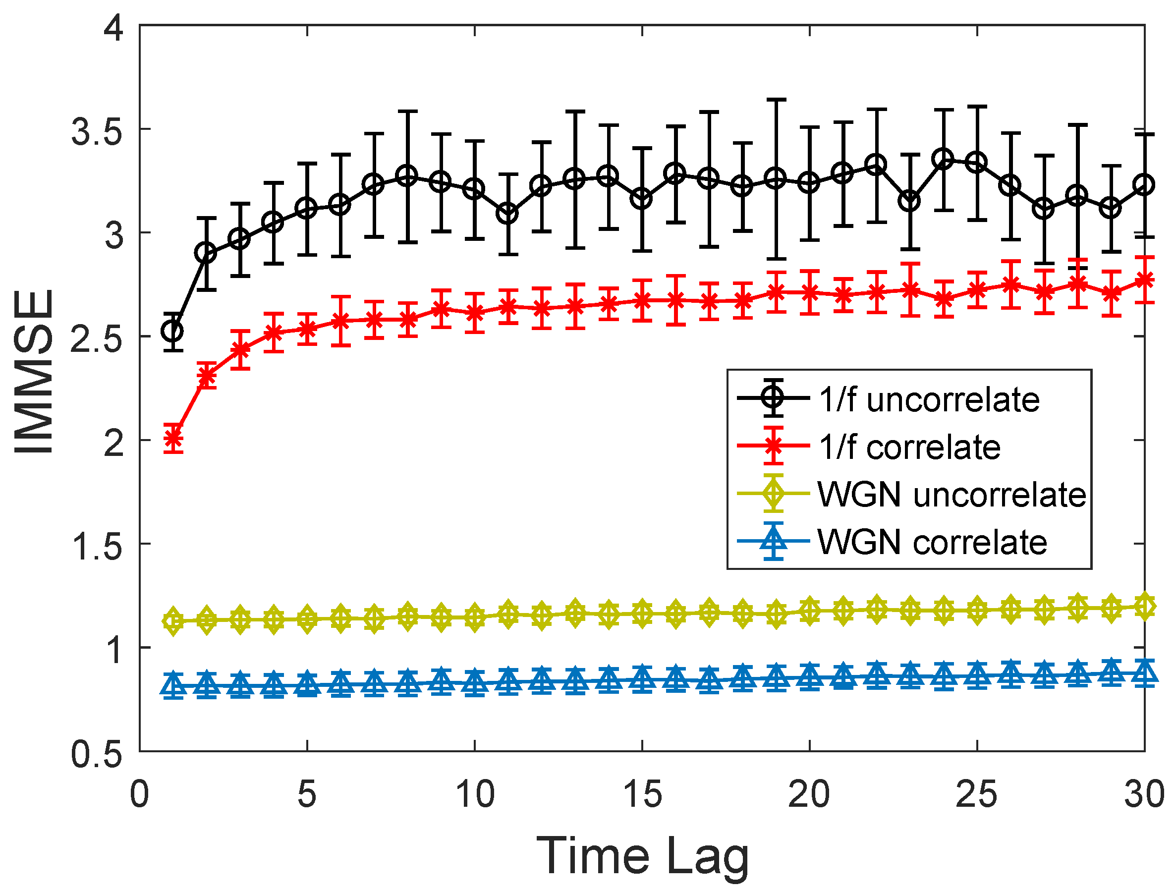
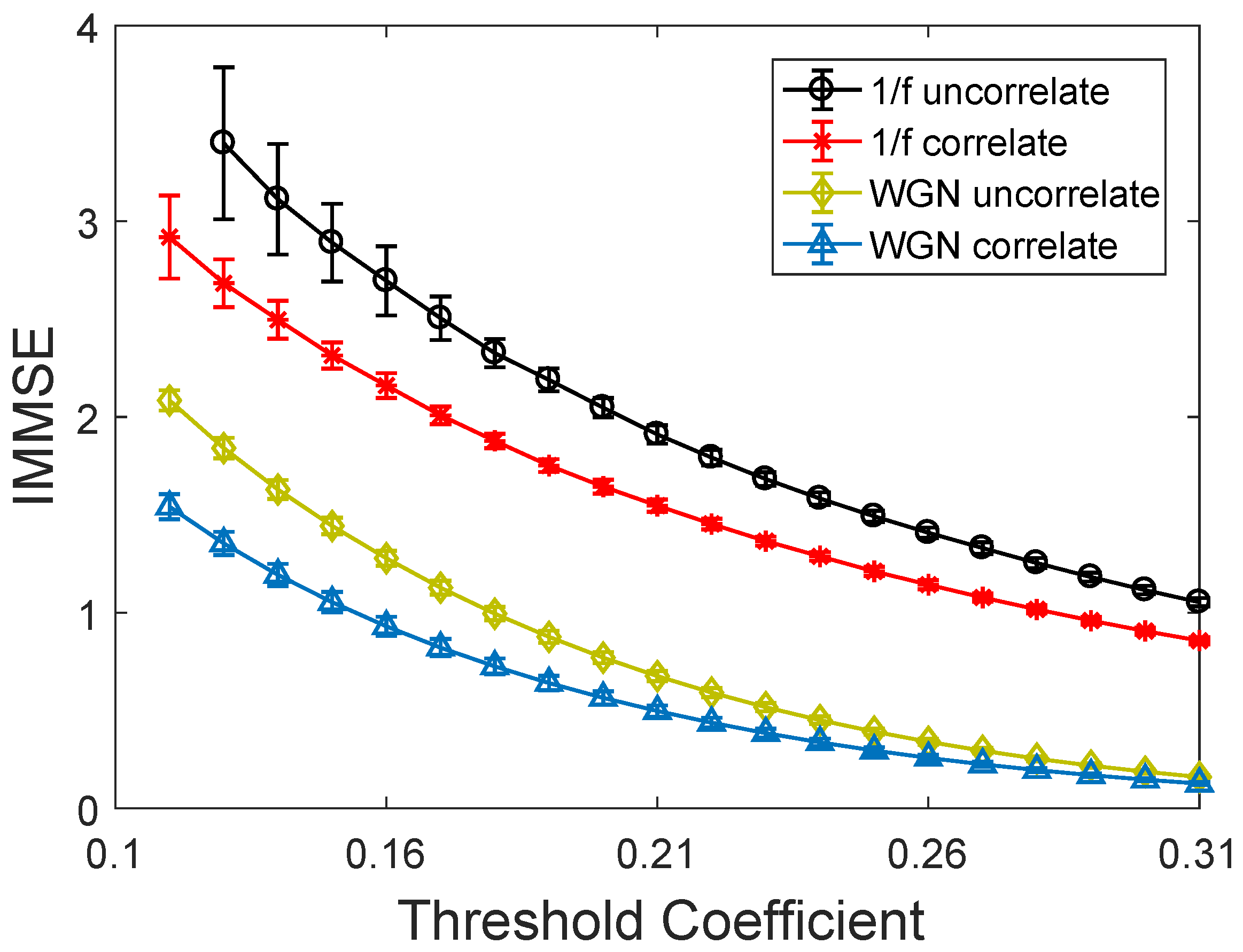
3.1. Parameter Selection

Compared to the traditional multivariate multiscale sample entropy algorithm, IMMSE can proficiently extract both within- and cross-channel information from the signal. Additionally, the algorithm exhibits robustness when processing complex real-world data. In this paper, our simulation analysis primarily focuses on studying the impact of various parameters on the stability of the IMMSE algorithm and its ability to extract cross-channel information. In this section, we first generate four sets of multi-channel data: correlated Gaussian white noise, uncorrelated Gaussian white noise, correlated 1 / f noise, and uncorrelated 1 / f noise. The IMMSE algorithm’s parameter selection range is studied using four different types of noise. The correlation information between the channels of the four types of simulated signals is shown in Figure 1 and Table 1. In Figure 1, the data length of each channel that was used for calculating the cross-correlation function is 10,000.
According to the definition of the coarse-graining process, the coarse-graining process involves dividing a time series into segments and calculating the mean of each segment. This implies that with an increase in temporal scale, the length of the coarse-grained data gradually decreases. Previous studies have indicated that the variation trends of entropy values at different temporal scales can reveal correlation information within signal channels [13]. However, data length can influence the stability of entropy values. To mitigate the impact of data length on the IMMSE results, we set the data length within each channel to be 50 k. The scale factor range is [ 1 , 100 ] . This means that when the scale factor is 100, each channel contains 1000 sample points. Since the IMMSE algorithm is a generalized extension of the multiscale sample entropy algorithm, we first refer to the parameter selection criteria of the multiscale sample entropy algorithm to determine the appropriate values for the remaining parameters [13]. Other parameters are set to be p = 3 , M = [ 2 , 2 , 2 ] , τ = [ 1 , 1 , 1 ] , and r = 0.15 .
Based on Figure 2, the following conclusions can be drawn. The variation in time scale has a negligible impact on the stability of IMMSE results because, with the scale factor increases, the standard deviations of the IMMSE curves are relatively stable. When distinguishing between the four different types of data involved in the simulation experiments, the overall trend of the curves allows for the differentiation of different signal types. However, it is essential to note that when the time scale exceeds 56, IMMSE cannot effectively differentiate between correlated and uncorrelated white noise. Additionally, with an increase in time scale, the standard deviation of IMMSE results for 1 / f noise gradually increases, while the standard deviation for white noise decreases. This phenomenon is attributed to the different within-channel correlations of the white noise and 1 / f noise.
Based on the results from Figure 2, we select a time scale ( n = 10 ) with significantly different entropy values, keeping other parameters constant, and vary the data length. We then compute the IMMSE results for four different types of multi-channel data. The result is displayed in Figure 3.
From the curves in Figure 3, it is evident that when the data length is too small (the coarse-grained data length less than 200), the results are unstable. As the data length gradually increases, the standard deviation of the IMMSE curve decreases. When the data length exceeds 1000, the influence of data length on result stability diminishes. Considering the results from both Figure 2 and Figure 3, it is advisable to take a comprehensive consideration when selecting the scale factor range and data length. Ensuring that the coarse-grained data length remains larger than 1000 at the maximum scale is recommended.
Before reconstructing the phase space, it is essential to determine the embedding dimension and time lag for each channel. Typically, when each channel observes the same system, the parameter selection for different channels is usually the same. If different channels observe distinct systems, then parameters for each channel need to be determined separately. There are two methods for parameter selection. The first method involves using specific methods to determine parameters, which can be effective when there is sufficient prior information about the target system [18]. The second method is empirical parameter selection based on experience, which is a practical approach in the absence of prior information. Setting parameters based on empirical experience is very common in entropy algorithms. Although entropy algorithms involve phase space reconstruction, and many methods have been proposed to determine suitable phase space reconstruction parameters [19,20,21], they often fail to achieve satisfactory results in practical applications. Therefore, algorithms such as multiscale sample entropy, MMSE, multiscale permutation entropy, and multivariate multiscale permutation entropy typically determine appropriate phase space reconstruction parameters through empirical validation in simulation experiments [11,12,13,14,17]. In this analysis, we compute the IMMSE results for different parameter selections, providing references for parameter choice in practical applications.
The results from Figure 4 and Figure 5 indicate that when the embedding dimension is small, the IMMSE results are stable and can effectively distinguish between different signals. As the embedding dimension increases, the standard deviation of the IMMSE results gradually increases. For 1 / f noise, when the embedding dimension exceeds 3, the IMMSE results cannot be computed. This is because a too-large embedding dimension leads to excessively long composite delay vectors, further causing C i M ( r ) , B i M ( r ) , or B M ( r ) to take on values of 0. Concerning time lag, an increase in time lag results in a larger standard deviation of the IMMSE results. However, different time lags have a relatively small impact on IMMSE. Therefore, for a completely unknown system, it is generally recommended to choose an embedding dimension of 2 or 3 and a default time lag of 1 when computing IMMSE.
From Figure 6, it can be observed that when r is small, the IMMSE entropy values are unstable. As r increases, the standard deviation of IMMSE gradually decreases, and the ability to differentiate between different signals weakens.
The threshold coefficient affects the sensitivity of the algorithm when determining whether vectors are similar. When the threshold coefficient r is small, more vectors in phase space are classified as dissimilar, which further leads to a decrease in C i M ( r ) and C i M + p ( r ) . When C i M ( r ) and C i M + p ( r ) are small, even small changes in C i M ( r ) and C i M + p ( r ) can have a significant impact on the final IMSE results. Conversely, when the threshold coefficient r is large, more vectors are classified as similar, causing C i M ( r ) and C i M + p ( r ) to increase. When C i M ( r ) and C i M + p ( r ) are large, changes in their values have a smaller effect on the final IMSE results. Therefore, when the threshold coefficient is small, the IMMSE algorithm performs better in distinguishing between different types of signals, but its variance increases. When the threshold coefficient is large, the algorithm’s ability to differentiate between signal types decreases, but its variance becomes smaller. Therefore, it is recommended to set the range for the threshold coefficient around 0.15.

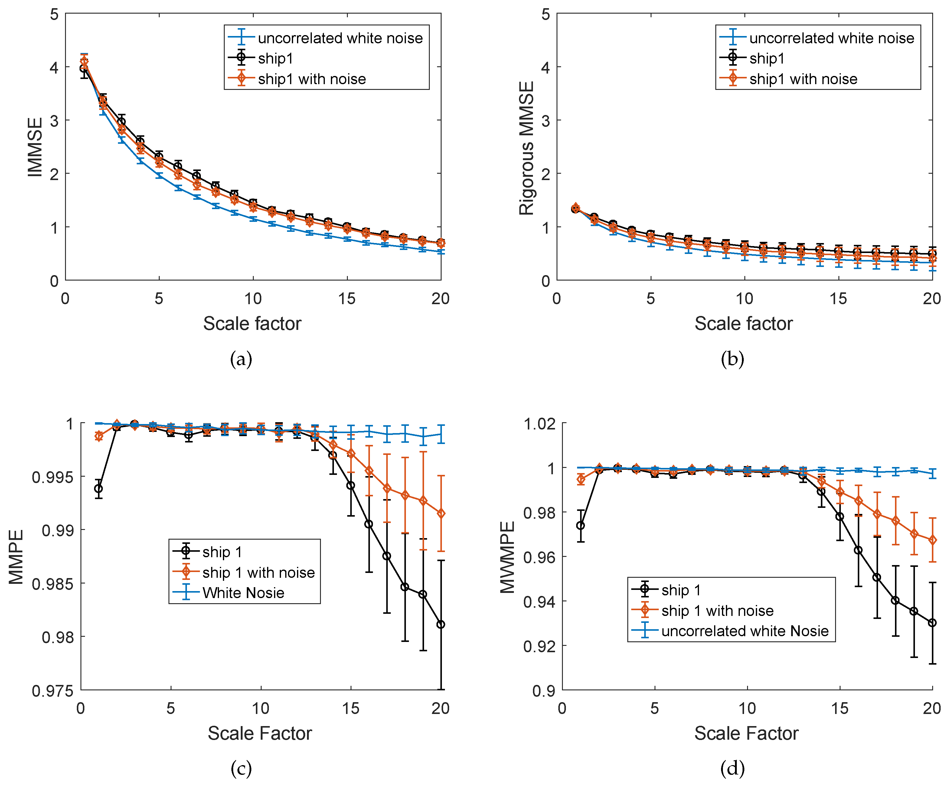
3.2. Noise Sensitivity Analysis

In the fields of underwater acoustic signal processing and mechanical fault diagnosis, noise inevitably affects the collected signals. The sensitivity of algorithms to noise directly influences the accuracy of subsequent detection and classification tasks. Since the target signals in these fields exhibit strong periodicity, we construct multi-channel continuous wave signals containing components of different frequencies. Gaussian white noise is then added to each channel of the generated multi-channel data, and the signal-to-noise ratio is adjusted. This study investigates the performance differences among the IMMSE, rigorous MMSE, and naive MMSE algorithms. The frequency components of the simulated signals are as follows: 20 Hz, 80 Hz, 250 Hz. Based on the previous parameter selection study, we set the data length of each channel as 5000, the embedding dimension M = [ 2 , 2 , 2 ] , the time lag τ = [ 1 , 1 , 1 ] , the threshold coefficient r = 0.15 , and the scale range as [ 1 , 20 ] . The signal-to-noise ratios are 10 dB, 5 dB, and 0 dB. The results are shown in Figure 7.
Based on the results in Figure 7, the rigorous MMSE algorithm is the least sensitive to noise. As the signal-to-noise ratio changes, the result curve of the rigorous MMSE algorithm shows little variation. In contrast, the IMMSE and naive MMSE algorithms exhibit similar curve structures under different signal-to-noise ratio conditions. This is because the main improvement of the IMMSE algorithm, compared to the naive MMSE algorithm, lies in its ability to extract cross-channel correlation information. However, since this set of simulations does not involve cross-channel correlation, there is no significant difference between the results of the two algorithms. From Figure 7a,c, it can be observed that the entropy curves of the continuous wave signals gradually approach the Gaussian white noise curve as the signal-to-noise ratio decreases, yet they still maintain similar structural features. Local minima are observed at scales 5, 10, 15, and 20. The consistent trend of the curve change indicates that both the IMMSE and naive MMSE algorithms can effectively reveal the complexity structure of the target signal in the time domain. In contrast, although the rigorous MMSE algorithm is less sensitive to noise, the curves under different signal-to-noise ratio conditions appear more chaotic, failing to accurately reveal the complexity structure of the signal in the time domain.

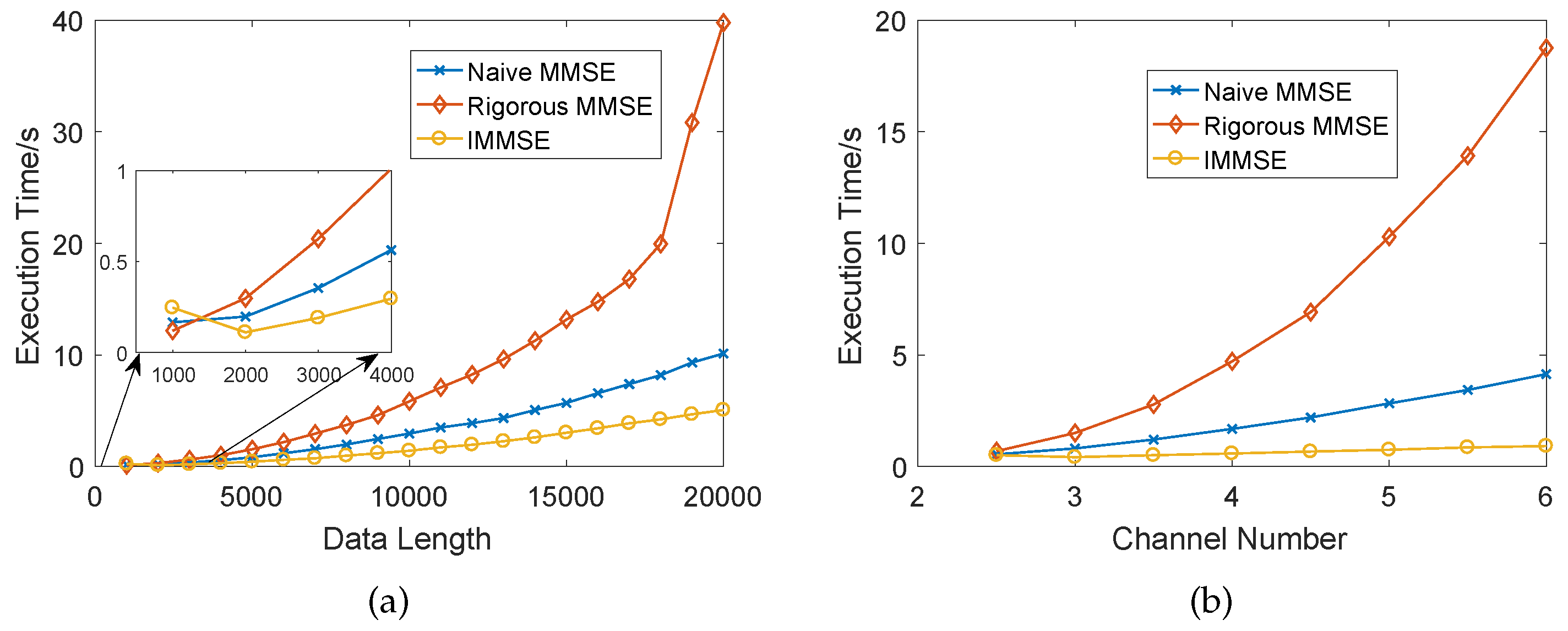
3.3. Computational Efficiency

The final set of simulations investigates the computational efficiency of different multi-channel entropy algorithms. First, three-channel Gaussian white noise is constructed, and the data length of each channel is gradually increased. The corresponding naive MMSE, rigorous MMSE, and IMMSE are then calculated. The parameters are M = [ 2 , 2 , 2 ] , τ = [ 1 , 1 , 1 ] , r = 0.15 , and the scale range is [ 1 , 20 ] . Furthermore, we fix the data length of each channel at 5000, keeping the other parameters unchanged, and gradually increase the number of channels. The computational efficiency of different algorithms is compared as the number of channels changes. The specific results are shown in Figure 8.
The results in Figure 8 demonstrate the computational efficiency of different multi-channel entropy algorithms. It is clear that, when the data length and number of channels are small, there is no significant difference in the computation speed of the three algorithms. However, as the data length and number of channels increase, the computational time of the rigorous MMSE and naive MMSE algorithms becomes significantly longer than that of the IMMSE algorithm. The rigorous MMSE algorithm not only has the slowest computation speed but also exhibits the fastest growth trend, meaning that as the number of channels or data length increases, the disadvantages of the rigorous MMSE algorithm become more apparent. In contrast, the IMMSE algorithm is the fastest, and its rate of change with increasing data length and channel number is the slowest. This is because, in the IMMSE algorithm, after increasing the embedding dimension, only a fixed phase space needs to be reconstructed. In contrast, both the rigorous MMSE and naive MMSE algorithms require the reconstruction of an increasing number of phase spaces as the number of channels grows. Even when the number of channels remains constant, increasing the data length results in the need to reconstruct more phase spaces, thereby increasing the computational burden of traditional MMSE algorithms.

4. Real-World Data Analysis

In this section, we analyze three different sets of real-world multi-channel data using the IMMSE algorithm. For complex real-world systems, it is challenging to determine appropriate phase space reconstruction parameters using traditional methods. Therefore, in this section we use the parameter selection range identified in the previous sections to calculate IMMSE and rigorous MMSE. We compare the performance of these two algorithms in processing real-world data. In this section, 20 independent repetitions of the experiment are conducted for data processing, and the corresponding error bar are generated.

4.1. Case 1

In the first set of real-world data analysis, the data we used is three-channel ship-radiated noise. The sample frequency is 9960 Hz. The parameters are M = [ 2 , 2 , 2 ] , τ = [ 1 , 1 , 1 ] , r = 0.15 . The original data length of each channel is 5000. We calculate the IMMSE results for this type of ship-radiated noise and three-channel uncorrelated white noise. Next, we add white noise into ship-radiated noise, ensure the signal-to-noise ratio (SNR) is 0 dB, and calculate the IMMSE result. The results are shown in Figure 9a. In Figure 9b, we computed the MMSE algorithm using a rigorous approach, with the same parameters as in Figure 9a. We also computed the multivariate multiscale permutation entropy (MMPE) and multivariate weighted multiscale permutation entropy (MWMPE) results for the same dataset. Referring to existing studies [22,23], the parameter settings for MMPE and MWMPE were embedding dimension 3, time delay 1, and scale range [ 1 , 20 ] .
The results from Figure 9a indicate that, under the original SNR conditions, the IMMSE algorithm effectively distinguishes between white noise and ship-radiated noise. Even when white noise is added, resulting in an SNR of 0 dB, IMMSE can still differentiate effectively between white noise and ship-radiated noise. The distinctiveness in cross-channel correlation information between ship-radiated noise and uncorrelated white noise arises from all channels observing the same system (the ship) during ship-radiated noise data collection. This inherent correlation among channels for ship-radiated noise is markedly different from the cross-channel correlation present in white noise. The IMMSE algorithm is proficient in capturing and utilizing this cross-channel correlation information, enabling effective differentiation between signals even in situations with low SNR. In contrast, the results from Figure 9b suggest that although the means of the three signals are similar to the IMMSE results, the excessively large standard deviation prevents the MMSE algorithm from effectively distinguishing between the signals. In Figure 9c,d, the results of MMPE and MWMPE exhibit characteristics completely opposite to those of IMMSE and rigorous MMSE, which are based on sample entropy. It is evident that when the scale is less than 13, MMPE and MWMPE fail to distinguish between different signal types. However, when the scale exceeds 13, both algorithms effectively differentiate between them. Moreover, the results of MMPE and MWMPE are similar, showing no significant differences. When dealing with shorter data lengths, where the scale range is constrained, the IMMSE algorithm maintains strong stability, allowing it to effectively distinguish different signal types.
Next, we analyze another set of real-world underwater acoustic data. Two types of data correspond to background noise and target echo signals, all collected during the same voyage. The sampling frequency is 256,000 Hz, and the number of channels is 3. The parameter settings remain consistent with Figure 9. The results are shown in Figure 10.
From Figure 10, it can be observed that all four entropy-based algorithms effectively distinguish different signal types. We compare two groups: sample entropy-based algorithms (IMMSE and rigorous MMSE), and permutation entropy-based algorithms (MMPE and MWMPE).
Comparing Figure 10a,b, the performance difference between IMMSE and rigorous MMSE is minimal. At lower scales, IMMSE exhibits higher variance, whereas at higher scales, rigorous MMSE has greater variance. Neither algorithm shows overlapping curves, confirming that both effectively differentiate signal types. We believe that this is due to minimal variation across channels during data acquisition, ensuring that cross-channel computations do not significantly impact algorithm stability. In contrast, comparing Figure 10c,d, we can observe that although the MMPE results exhibit similar trends for the two curves, the algorithm’s stability allows it to effectively distinguish different types of signals. However, from an overall perspective, the results based on sample entropy demonstrate better signal differentiation compared to those based on permutation entropy.

4.2. Case 2

In the second set of simulation experiments, we used data from Southeast University gear dataset [24]. The dataset includes three categories of three-channel gear signals: chipped tooth (Chipped), health working state (Health), surface fault (Surface). Each set of signals was recorded under the working condition of 20 Hz (1200 rpm)–0 V (0 Nm) load. Each category of signal consists of three-channel data representing the vibrations of a planetary gearbox in the x , y , and z directions. The parameters are M = [ 2 , 2 , 2 ] , τ = [ 1 , 1 , 1 ] , r = 0.15 ; the original data length of each channel is 5000. The rigorous MMSE and IMMSE results are shown in Figure 11.
From the curves of the two algorithms in Figure 11, it can be seen that the IMMSE algorithm is significantly more stable than the rigorous MMSE algorithm when processing actual complex signals, effectively distinguishing between the three different signals. Additionally, for the Health signal curve, the IMMSE algorithm preserves the structural characteristics of the signal across different time scales (showing a decline from scale 1 to 3, and a noticeable upward trend from scale 3 to 14 compared to the other two signals).

4.3. Case 3

In the third set of simulation experiments, we used bearing data obtained from Southeast University bearing dataset [24]. The dataset includes three categories of three-channel gear signals: ball fault (Ball), health working state (Health), outer ring fault (Outer). Each set of signals was recorded under the working condition of 20 Hz (1200 rpm)–0 V (0 Nm) load. Each category of signal consists of three-channel data representing the vibrations of a parallel gearbox in the x , y , and z directions. The parameters are M = [ 2 , 2 , 2 ] , τ = [ 1 , 1 , 1 ] , r = 0.15 ; the original data length of each channel is 5000. The rigorous MMSE and IMMSE results are shown in Figure 12.
In the results of Figure 12, the IMMSE results are more stable compared to the rigorous MMSE results. The trend of the IMMSE for the three types of signals is also similar to the MMSE results, showing a clear decreasing trend when the scale is less than 10 and stabilizing when the scale is greater than 10. The smaller variance allows for effective differentiation of different types of fault signals using IMMSE.

5. Conclusions

Addressing the challenge of parameter selection in practical applications, this paper provides a parameter selection range for analyzing unknown systems. When calculating IMMSE, the temporal scale should be less than 56. The coarse-grained data length remaining larger than 1000 is recommended. The embedding dimension should be 2 or 3 for each channel, and time lag for each channel is recommended to be 1. The range of the threshold coefficient r should be around 0.15 . The comparative study between the IMMSE algorithm and traditional MMSE algorithms demonstrates that the IMMSE algorithm can effectively extract the complexity features of multi-channel data in the time-domain structure, while maintaining a relatively low computational cost as the data length and number of channels increase.
The analysis of real-world data shows that, when processing multi-channel underwater acoustic data, the IMMSE algorithm can effectively improve the subsequent classification accuracy through neural networks due to its greater stability. Even when the signal-to-noise ratio is reduced to 0 dB, the IMMSE algorithm can still effectively distinguish between signal and noise, demonstrating its strong noise resilience. In contrast, the rigorous MMSE algorithm, with its excessively large variance, causes overlapping error curves, leading to lower classification accuracy. Furthermore, this paper also analyzes different types of mechanical fault signals, and the results show that IMMSE outperforms the rigorous MMSE algorithm, proving that IMMSE has broad applicability.

Author Contributions

J.Z., Y.L. and M.W. conceived and designed the research. J.Z. analyzed the data and wrote the manuscript. Y.L. and M.W. revised the manuscript. All authors have read and agreed to the published version of the manuscript.

Funding

This work is supported by the fund of National Key Laboratory of Underwater Information and Control.

Data Availability Statement

The datasets analyzed during the current study are available from the corresponding author on reasonable request.

Conflicts of Interest

The authors declare no conflict of interest.

References

  1. Macek, W.M. Nonlinear dynamics and complexity in the generalized Lorenz system. Nonlinear Dyn. 2018, 94, 2957–2968. [Google Scholar] [CrossRef]
  2. Sharma, A.; Patidar, V.; Purohit, G.; Sud, K.K. Effects on the bifurcation and chaos in forced Duffing oscillator due to nonlinear damping. Commun. Nonlinear Sci. Numer. Simul. 2012, 17, 2254–2269. [Google Scholar]
  3. Li, H.; Shen, Y.; Han, Y.; Dong, J.; Li, J. Determining Lyapunov exponents of fractional-order systems: A general method based on memory principle. Solitons Fractals 2023, 168, 113167. [Google Scholar]
  4. Siddagangaiah, S.; Chen, C.; Hu, W.; Farina, A. The dynamical complexity of seasonal soundscapes is governed by fish chorusing. Commun. Earth Environ. 2022, 3, 109. [Google Scholar] [CrossRef]
  5. Patel, P.; Raghunandan, R.; Annavarapu, R. EEG-based human emotion recognition using entropy as a feature extraction measure. Brain Inf. 2021, 8, 20. [Google Scholar]
  6. Wiercigroch, M.; Badiey, M.; Simmen, J.; Cheng, A.D. Non-linear dynamics of underwater acoustics. J. Sound Vib. 1999, 220, 771–786. [Google Scholar]
  7. Wiercigroch, M.; Cheng, A.H.D.; Simmen, J.; Badiey, M. Nonlinear behavior of acoustic rays in underwater sound channels. Chaos Solitons Fractals 1998, 9, 193–207. [Google Scholar]
  8. Li, Y.; Gao, P.; Tang, B.; Yi, Y.; Zhang, J. Double feature extraction method of ship-radiated noise signal based on slope entropy and permutation entropy. Entropy 2021, 24, 22. [Google Scholar] [CrossRef]
  9. Li, Y.; Tang, B.; Yi, Y. A novel complexity-based mode feature representation for feature extraction of ship-radiated noise using VMD and slope entropy. Appl. Acoust. 2022, 196, 108899. [Google Scholar]
  10. Li, W.; Shen, X.; Li, Y. A comparative study of multiscale sample entropy and hierarchical entropy and its application in feature extraction for ship-radiated noise. Entropy 2019, 21, 793. [Google Scholar] [CrossRef]
  11. He, Y.; Huang, J.; Zhang, B. Approximate entropy as a nonlinear feature parameter for fault diagnosis in rotating machinery. Meas. Sci. Technol. 2012, 23, 045603. [Google Scholar] [CrossRef]
  12. Richman, J.S.; Moorman, J.R. Physiological time-series analysis using approximate entropy and sample entropy. Am. J. Physiol. Heart Circ. Physiol. 2000, 278, H2039–H2049. [Google Scholar] [CrossRef] [PubMed]
  13. Costa, M.; Goldberger, A.L.; Peng, C.K. Multiscale entropy analysis of complex physiologic time series. Phys. Rev. Lett. 2002, 89, 068102. [Google Scholar] [CrossRef] [PubMed]
  14. Ahmed, M.U.; Mandic, D.P. Multivariate multiscale entropy analysis. IEEE Signal Process. Lett. 2012, 19, 91–94. [Google Scholar] [CrossRef]
  15. Cao, L.; Mees, A.; Judd, K. Dynamics from multivariate time series. Physical D 1998, 121, 75–88. [Google Scholar] [CrossRef]
  16. Yin, Y.; Shang, P. Multivariate multiscale sample entropy of traffic time series. Nonlinear Dyn. 2016, 86, 479–488. [Google Scholar] [CrossRef]
  17. Li, W.; Shen, X.; Li, Y.; Chen, Z. Improved multivariate multiscale sample entropy and its application in multi-channel data. Chaos 2023, 33, 6. [Google Scholar] [CrossRef]
  18. Lang, S.; Zhu, H.; Sun, G.; Jiang, Y.; Wei, C. A study on methods for determining phase space reconstruction parameters. J. Comput. Nonlinear Dyn. 2022, 17, 011006. [Google Scholar] [CrossRef]
  19. Ma, H.; Han, C. Selection of embedding dimension and delay time in phase space reconstruction. Front. Electr. Electron. Eng. China 2006, 1, 111–114. [Google Scholar] [CrossRef]
  20. Kennel, M.B.; Brown, R.; Abarbane, H.D.I. Determining embedding dimension for phase-space reconstruction using a geometrical construction. Phys. Rev. A 1992, 45, 3403. [Google Scholar] [CrossRef]
  21. Matilla-García, M.; Morales, I.; Rodríguez, J.M.; Ruiz Marín, M. Selection of embedding dimension and delay time in phase space reconstruction via symbolic dynamics. Entropy 2021, 23, 221. [Google Scholar] [CrossRef] [PubMed]
  22. Morabito, F.C.; Labate, D.; Foresta, F.L.; Bramanti, A.; Morabito, G.; Palamara, I. Multivariate multi-scale permutation entropy for complexity analysis of Alzheimer’s disease EEG. Entropy 2012, 14, 1186–1202. [Google Scholar] [CrossRef]
  23. Yin, Y.; Shang, P. Multivariate weighted multiscale permutation entropy for complex time series. Nonlinear Dyn. 2017, 88, 1707–1722. [Google Scholar]
  24. Zhang, X.; Zhang, S.; Dong, W.; Song, S.; Wang, K. Method for locating single-phase disconnection faults in a smart distribution system based on refined composite multiscale permutation q-complexity entropy and random forest. IEEE Sens. J. 2023, 23, 11925–11935. [Google Scholar]
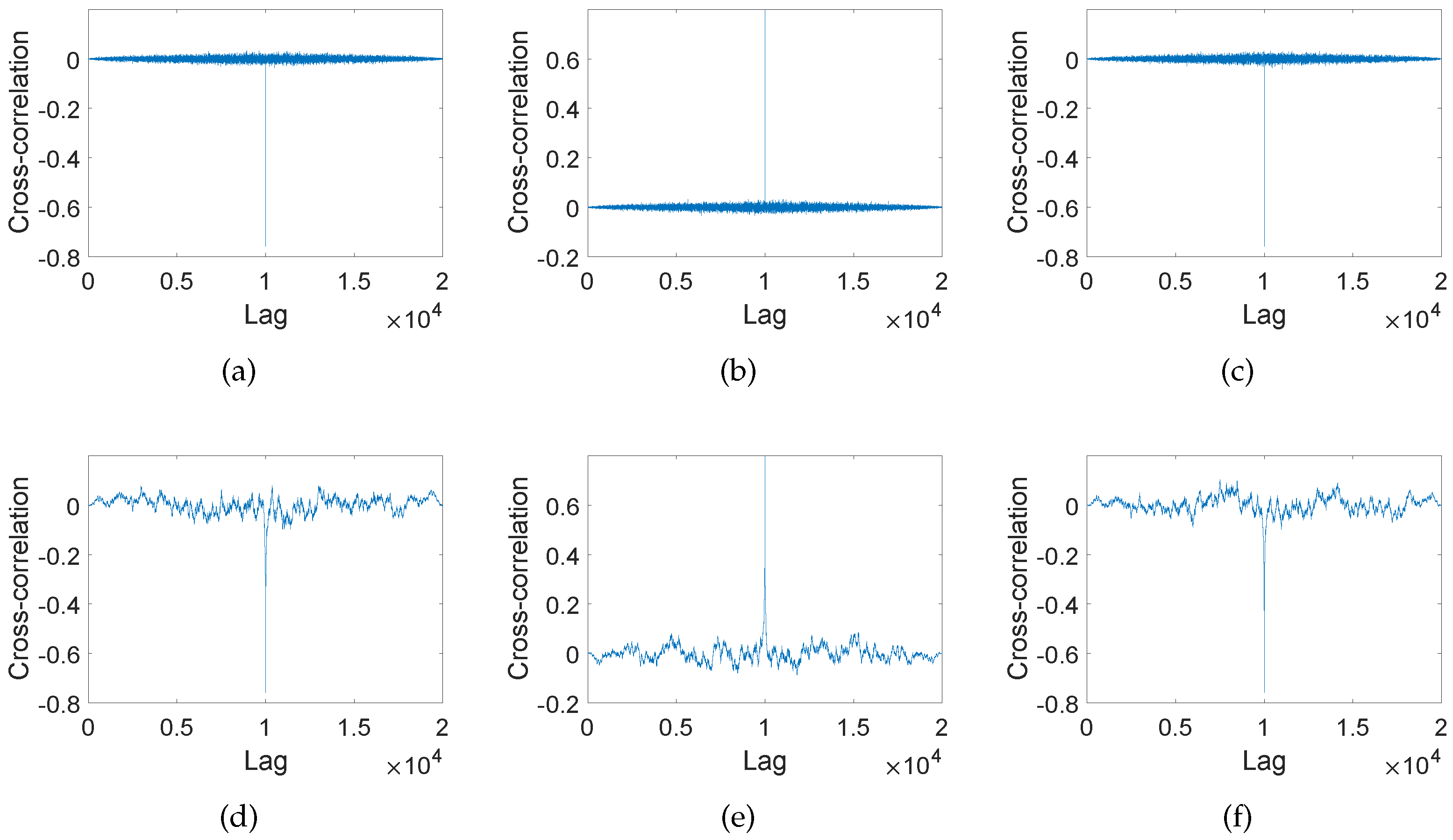
Figure 1. Cross-correlation information of simulated multi-channel datasets. (a) Cross-correlation of Gaussian white noise between channel 1 and 2. (b) Cross-correlation of Gaussian white noise between channel 2 and 3. (c) Cross-correlation of Gaussian white noise between channel 1 and 3. (d) Cross-correlation of 1 / f noise between channel 1 and 2. (e) Cross-correlation of 1 / f noise between channel 2 and 3. (f) Cross-correlation of 1 / f noise between channel 1 and 3.
Jmse 13 00675 g001
Figure 2. IMMSE results for correlated and uncorrelated multi-channel signals. The scale factor range is from [ 1 , 100 ] .
Jmse 13 00675 g002
Figure 3. The scale factor is n = 10 . IMMSE results for correlated and uncorrelated multi-channel signals. The data length range is from [ 100 , 2600 ] . This means that the range of original data length is [1000, 26,000].
Jmse 13 00675 g003
Figure 4. The scale factor is n = 10 . IMMSE results for correlated and uncorrelated multi-channel signals. The range of the embedding dimension is [ 2 , 10 ] . Original data length is 50 k, r = 0.15 , τ = [ 1 , 1 , 1 ] .
Jmse 13 00675 g004
Figure 5. The scale factor is n = 10 . IMMSE results for correlated and uncorrelated multi-channel signals. The range of the time lag is [ 1 , 30 ] . Original data length is 10 k, r = 0.15 , M = [ 2 , 2 , 2 ] .
Jmse 13 00675 g005
Figure 6. The scale factor is n = 10 . IMMSE results for correlated and uncorrelated multi-channel signals. The range of the threshold coefficient r is [ 0.1 , 0.3 ] . Data length is 10 k, M = [ 2 , 2 , 2 ] , τ = [ 1 , 1 , 1 ] .
Jmse 13 00675 g006
Figure 7. Study on the noise sensitivity of different algorithms. (a) IMMSE algorithm. (b) Rigorous MMSE algorithm. (c) Naive MMSE algorithm.
Jmse 13 00675 g007
Figure 8. The computational efficiency of different multivariate entropy algorithms. (a) Execution times of multivariate entropy algorithms for different data lengths in each channel. (b) Execution times of different multivariate entropy algorithms with varying numbers of channels.
Jmse 13 00675 g008
Figure 9. Entropy results for multi-channel ship-radiated noise. (a) IMMSE results for real-world ship-radiated noise and ambient noise. (b) Rigorous MMSE results for real-world ship-radiated noise and ambient noise. (c) MMPE results for real-world ship-radiated noise and ambient noise. (d) MWMPE results for real-world ship-radiated noise and ambient noise.
Jmse 13 00675 g009
Figure 10. Entropy results for different types of multi-channel underwater acoustic signals. (a) IMMSE results. (b) Rigorous MMSE results. (c) MMPE results. (d) MWMPE results.
Jmse 13 00675 g010
Figure 11. Entropy results for multi-channel gear vibration signal. (a) IMMSE results for real-world gear vibration signal. (b) Rigorous MMSE results for real-world gear vibration signal.
Jmse 13 00675 g011
Figure 12. Entropy results for multi-channel bearing vibration signal. (a) IMMSE results for real-world bearing vibration signal. (b) Rigorous MMSE results for real-world bearing vibration signal.
Jmse 13 00675 g012
Table 1. The numerical results of the cross-correlation between channels of the simulated signals (Ch.1/2/3 is the abbreviation for Channel 1/2/3).
Gaussian White Noise 1 / f Noise
Ch.1Ch.2Ch.3Ch.1Ch.2Ch.3
Ch.11.0000−0.7589−0.75891.0000−0.7589−0.7589
Ch.2−0.75891.00000.8000−0.75891.00000.8000
Ch.3−0.75890.80001.0000−0.75890.80001.0000
Disclaimer/Publisher’s Note: The statements, opinions and data contained in all publications are solely those of the individual author(s) and contributor(s) and not of MDPI and/or the editor(s). MDPI and/or the editor(s) disclaim responsibility for any injury to people or property resulting from any ideas, methods, instructions or products referred to in the content.

