A Study of a Nonsmooth Fuzzy Active Disturbance Rejection Control Algorithm for Gas Turbines in Maritime Autonomous Surface Ship

Abstract

To address the dynamic and robust performance limitations of gas turbines in maritime autonomous surface ship applications, this paper proposes a novel nonsmooth fuzzy active disturbance rejection control (NS_FADRC) algorithm. This method combines the strengths of linear active disturbance rejection control (LADRC), nonsmooth control, and fuzzy adaptive control. First, the extended state observer (ESO) is improved by using the nonsmooth control method to enhance its convergence rate and estimation capability, while ensuring finite-time convergence characteristics. Next, fuzzy control logic is integrated to enhance the adaptability of the state error feedback (SEF), overcoming the limitations of traditional SEF in handling nonlinearities. The stability of the proposed control algorithm is further validated using Lyapunov stability analysis. Lastly, a Hardware-in-the-Loop (HIL) semi-physical simulation platform, based on automatic code generation technology, is developed to validate the algorithm’s performance. Experimental results demonstrate that, compared to the PID, FPID, and LADRC algorithms, the proposed NS_FADRC algorithm provides superior dynamic response during speed step tracking and excellent robust disturbance rejection performance in the presence of load disturbances, parameter uncertainties, and measurement noise.

1. Introduction

With the advancement of economic globalization, oceanic domains have become critical to national energy security and economic sustainability [1,2]. Maritime Autonomous Surface Ship (MASS), characterized by their high autonomy and intelligence, are emerging as transformative technologies for maritime exploration and industry development [3,4]. Gas turbines, known for their excellent dynamic performance [5,6], quiet operation [7], compact structure, and high power density [8], hold considerable potential for application in the MASS field.

For the MASS, superior maneuverability and operational stability are key performance indicators. High-mobility conditions such as automatic obstacle avoidance and accelerated pursuit can impose significant impacts on the MASS’s electrical system, which manifest as frequent variations in the load power at the engine end. Speed control is a critical component of the gas turbine control system, directly influencing the turbine’s dynamic performance, reliability, lifespan, and power quality [9]. The speed controller must maintain minimal speed fluctuations under steady-state conditions, minimize overshoot during external disturbances or sudden load changes, and enable the system to quickly return to a stable state. Therefore, the optimization of gas turbine speed control is essentially a multi-objective optimization and trade-off problem between fast response and stability.

The proportional-integral-derivative (PID) control method is widely used in gas turbines due to its simplicity, clear physical significance, ease of implementation, and robustness. As a linear controller, the PID typically linearizes the controlled system under the design operating conditions and tunes the control parameters based on classical control theory [10]. However, the controller gain parameters that are tuned for specific operating conditions may not provide optimal control performance across the full operating range. Furthermore, under varying external conditions, large-scale load fluctuations, or the degradation of gas turbine components, pre-tuned parameters may result in degraded control performance or even engine instability. The unique characteristics of MASS prevent the on-site tuning of the gas turbine control system, thereby reducing the reliability of unmanned gas turbine units during long-range operations.

With the advancement of modern intelligent control theories, sophisticated algorithms including neural networks, model predictive control (MPC), and sliding mode control have been increasingly implemented to enhance gas turbine speed control systems. Iqbal et al. [11] developed a fuzzy rule-based PID parameter adaptation strategy to mitigate instability in grid-connected gas turbines under load fluctuations. Similarly, Li et al. [12] utilized fuzzy adaptive PID control to suppress overspeed phenomena during load shedding in turbine-generator systems. Nevertheless, the design of effective fuzzy adjustment mechanisms presents significant challenges, requiring the meticulous selection of membership functions and rule formulation that heavily depends on engineering expertise. While neural network-enhanced PID methods [13,14,15] demonstrate adaptive parameter tuning capabilities, their practical implementation is constrained by computational complexity and slow convergence rates, rendering them unsuitable for real-time parameter adaptation.

In the realm of model-based approaches, Jurado et al. [16] employed linearized MPC to improve generator set stability, though its effectiveness remains restricted to linear operating regimes. Subsequent innovations by Saez et al. [17] introduced genetic algorithm-optimized fuzzy predictive control to address nonlinear system challenges, while Haji et al. [18] proposed adaptive MPC with online parameter estimation. However, the intricate model structures and substantial computational demands that are inherent to nonlinear MPC implementations hinder their widespread engineering adoption.

Robust control strategies have emerged as alternative solutions, with Ariffin et al. [19] employing an $H_{\infty }$ control method to counteract manufacturing tolerance impacts, and Gomma et al. [20] designing state-space robust controllers with anti-windup compensation. Najimi et al. [21] further advanced this domain through linear autoregressive robust control design. These methods, however, typically exhibit conservatism in control performance, where robustness improvements necessitate trade-offs in dynamic responsiveness.

The active disturbance rejection control (ADRC) algorithm integrates classical control theory with modern control methods. Unlike traditional control approaches, ADRC does not rely on an accurate system model but treats unmodeled dynamics and uncertainties as disturbances, effectively addressing the limitations of model-dependent modern control methods. This makes ADRC particularly suitable for gas turbine speed control in MASS. In reference [22], an ADRC algorithm was designed for a micro gas turbine generator system, which demonstrated a faster dynamic response compared to PID control.

Wang et al. [23] employed deep reinforcement learning to optimize the ADRC algorithm, achieving the self-adaptive tuning of its gain parameters. Chen et al. [24] integrated fractional-order theory into the ADRC framework, demonstrating enhanced transient response characteristics. Furthermore, Yue et al. [25] proposed an improved ADRC algorithm based on an adaptive unscented Kalman filter (AUKF). The results demonstrated that this algorithm can improve both the system’s response speed and its robustness against unknown disturbances.

Despite these advancements, conventional ADRC implementations face industrial adoption barriers due to their reliance on multiple nonlinear functions that complicate parameter tuning and theoretical analysis. To address this, Gao [26] pioneered linear ADRC (LADRC) through bandwidth-based simplification, significantly advancing industrial applications. However, LADRC exhibits inherent limitations when applied to highly nonlinear systems like gas turbines, manifesting as inadequate disturbance estimation accuracy and poor adaptability to operational uncertainties, ultimately compromising control performance.

Motivated by the foregoing discussions, this paper proposes a novel nonsmooth fuzzy ADRC method for gas turbines, based on an adaptive disturbance rejection mechanism. Compared to existing studies, the novelty and contributions of this paper can be summarized in the following three aspects:

(1) A new control technique is proposed that combines nonsmooth theory, fuzzy adaptive control theory, and LADRC theory. This method organically integrates the advantages of all three methodologies, is model-independent, and allows for easy parameter tuning. It also demonstrates superior dynamic response and robustness, overcoming the limitations of traditional PID control, the heavy reliance on models in modern control methods, and the inadequate disturbance estimation and adaptability of conventional ADRC methods.

(2) Unlike conventional ESO [20,22], a novel nonsmooth ESO (NS_ESO) is designed for disturbance estimation, which effectively improves estimation accuracy and speed by replacing the linear function with a nonsmooth function, ensuring the finite-time convergence of the ESO.

(3) Fuzzy adaptive control is incorporated as an optimization mechanism into the control strategy. The optimization focuses on designing a new adaptive control law based on a fuzzy logic controller, enabling the real-time adjustment of PD controller parameters based on error and error-derivative signals, thereby further enhancing the robustness and response speed of the controller.

The rest of this article is organized as follows. Section 2 introduces the design process of the NS_FADRC method. Section 3 details the stability analysis process of NS_FADRC. Section 4 presents the corresponding experimental results. Finally, Section 5 concludes this article.

2. Design of the NS_FADRC Method

The design of the observer and the stability analysis of the controller require referencing the dynamic model of the controlled object. The micro gas turbine is a typical single-input single-output (SISO) system, where the input variable is the fuel flow rate, and the output variable is the speed signal. It can be simplified to a second-order nonlinear system as shown in Equation (1).

$$\left\{\begin{array}{l}{\dot{x}}_1(t)=x_2(t)\\ {\dot{x}}_2(t)=f\left(x_1(t),x_2(t)\right)+d(t)+bu\\ y(t)=x_1(t)\end{array}\right.(t)$$

(1)

where $u(t)$ and $y(t)$ represent the fuel flow input and speed output of the gas turbine, respectively. $d(t)$ is the external disturbance, and $f(x_1(t),x_2(t))$ denotes the complex nonlinear part of the system. b is the system gain, and its estimated value is defined as b₀.

By treating the system’s unknown nonlinearities as internal disturbances and expanding the total disturbance $d_{total}(t)=f(x_1(t),x_2(t))+d(t)$ into state variable $x_3$, Equation (1) can be rewritten as:

$$\left\{\begin{array}{l}\dot{\chi }(t)=A_E\chi (t)+B_E\overline{u}(t)+B_{E\tau }{\dot{d}}_{total}(t)\hfill \\ y(t)=C_E\chi (t)+D_E\overline{u}(t)\hfill \end{array}\right.$$

(2)

where $\chi (t)={[\begin{array}{ccc}{x}_1(t)& x_2(t)& x_3(t)\end{array}]}^T$ is the expanded state variable matrix, and ${\dot{d}}_{total}(t)$ represents the differential of the total disturbance. $\overline{u}(t)=bu(t)$, $B_E={\left[\begin{array}{ccc}0& 1& 0\end{array}\right]}^{\mathrm{T}}$, $B_{E\tau }={\left[\begin{array}{ccc}0& 0& 1\end{array}\right]}^{\mathrm{T}}$, $C_E=\left[\begin{array}{ccc}1& 0& 0\end{array}\right]$, $D_E=0$, $A_E=\left[\begin{array}{ccc}0& 1& 0\\ 0& 0& 1\\ 0& 0& 0\end{array}\right]$.

2.1. Tracking Differentiator

The tracking differentiator (TD) is designed to smooth out sharp variations in the input signal, reduce initial errors, and address the trade-off between overshoot and response speed. The discrete mathematical model of the TD is shown as follows:

$$\begin{array}{l}{r}_1(t+1)=r_1(t)+T\cdot r_2(t)\\ r_2(t+1)=r_2(t)+T\cdot \mathrm{fst}(r_1(t)-r(t),r_2(t),\delta ,d)\end{array}$$

(3)

where $r(t)$ is the reference input signal of the controller, $r_1(t)$ is the tracking signal of $r(t)$, $r_2(t)$ is the derivative signal of $r_1(t)$, $T$ is the time step, and $\mathrm{fst}(\cdot )$ is the rapid control synthesis function.

The function $\mathrm{fst}(\cdot )$ can be represented as:

$$\begin{array}{l}\mathrm{fst}(x_1(t),x_2(t),\delta ,h)=-\left\{\begin{array}{c}\delta \cdot a(t)/d,\left|a(t)\right|\le d\\ \delta \cdot \mathrm{sign}(a(t)),\left|a(t)\right|>d\end{array}\right.\\ \left\{\begin{array}{l}d=\delta \cdot h\hfill \\ d_0=d\cdot h\hfill \\ y(t)=x_1(t)+T\cdot x_2(t)\hfill \\ a_0(t)=\sqrt{d^2+8\cdot \delta \cdot \left|y(t)\right|}\hfill \\ a(t)=\left\{\begin{array}{l}{x}_2(t)+\left(a_0(t)-d\right)/2,\left|y(t)\right|>d_0\hfill \\ x_2(t)+y(t)/h,\left|y(t)\right|\le d_0\hfill \end{array}\right.\hfill \end{array}\right.\end{array}$$

(4)

where $\delta$ is the convergence rate coefficient, and $h$ is the filtering factor.

2.2. Design of the Nonsmooth Extended State Observer

2.2.1. Linear Extended State Observer

The extended state observer is a core component of the ADRC system. It provides estimates of the internal dynamics of the controlled object and can also eliminate the adverse effects of noise on the control system. For the second-order system shown in Equation (1), a linear extended state observer (LESO) can be designed as shown in the following expression.

$$\left\{\begin{array}{ll}\stackrel{.}{Z}(t)=A_{E}Z(t)+B_E\overline{u}(t)+L_o(y(t)-\widehat{y}(t))\hfill & \hfill \\ \widehat{y}(t)=C_{E}Z(t)+D_E\overline{u}(t)\hfill & \hfill \end{array}\right.$$

(5)

where $Z(t)={\left[\begin{array}{ccc}{z}_1(t)& z_2(t)& z_3(t)\end{array}\right]}^{\mathrm{T}}$, coefficient matrices $A_E$, ${{\rm B}}_E$, $C_E$, and $D_E$ are the same as Equation (2), and $L_0=\mathrm{diag}(l_1,l_2,l_3)$ is the observer gain matrix.

As shown in Equation (5), as long as the observer gain parameters $l_1$, $l_2$, and $l_3$ are selected appropriately, the changes in the system’s state variables can be effectively observed. However, the impact of these parameters on the observer’s performance still lacks universal research results to support it. Simply using a trial-and-error method can lead to low computational efficiency. Gao [21] proposed a new method to easily determine these parameters. This method uses the concept of bandwidth to approximate the determination of the gain parameters of the LESO.

Subtracting the expanded state system (2) from the designed LESO yields the observation error equation:

$${\dot{e}}_0(t)=\left(A_E-L_o{C}_E\right)e_0(t)+B_{E\tau }{\dot{d}}_{total}(t)$$

(6)

where $e_0(t)=\chi (t)-Z(t)$ represents the observation error matrix.

The stability of the above observation error equation depends on the matrix $A_E-L_o{C}_E$. Setting $A_{e0}=A_E-L_o{C}_E$ yields:

$$A_{e0}=A_E-L_o{C}_E=\left[\begin{array}{ccc}-l_1& 1& 0\\ -l_2& 0& 1\\ -l_3& 0& 0\end{array}\right]$$

(7)

The characteristic polynomial of the above equation can be expressed as:

$$Det(A_{e0})=\left|sI-A_{e0}\right|=s^3+l_1{s}^2+l_{2}s+l_3$$

(8)

Defining ${\omega }_0$ as the bandwidth of the observer, and placing all the eigenvalues of the characteristic polynomial at $-{\omega }_0$, we obtain:

$$s^3+l_1{s}^2+l_{2}s+l_3={(s+{\omega }_0)}^3$$

(9)

The value of the observer gain parameters can be calculated based on the observer bandwidth ${\omega }_0$.

$$\begin{array}{l}{l}_1=3{\omega }_0\\ l_2=3{\omega }_0^2\\ l_3={\omega }_0^3\end{array}$$

(10)

By using ${\omega }_0$, the number of undetermined parameters in the observer system is reduced from three to one, simplifying the parameter tuning process of the ESO. Moreover, in practical applications, ${\omega }_0$ has a clear physical meaning and fully reflects its physical characteristics and essence. This is one of the key reasons why a bandwidth-based ESO has been increasingly adopted and promoted by engineers in recent years.

2.2.2. Nonsmooth Extended State Observer

For ESOs, the convergence speed is a key performance indicator that determines their control accuracy. The LESO can only achieve asymptotic convergence, meaning the time for the observer to converge to the equilibrium point is infinite. Additionally, due to the complexity of gas turbine systems, the traditional LESO struggles to accurately estimate all unknown disturbances. In contrast, nonlinear extended state observers (NESOs) offer higher estimation accuracy and better transient performance. However, the large number of gain parameters in NESOs makes parameter tuning more challenging. Nonsmooth control, which refers to control forms involving fractional powers, typically offers better transient performance, robustness, and finite-time stability. On the other hand, nonsmooth control theory only adds a single exponent compared to traditional linear control, and its fewer adjustable gain parameters have made it a popular approach among many researchers. To improve the convergence speed of the ESO, this paper combines nonsmooth control (NSC) theory with the linear extended state observer to construct a nonsmooth extended state observer (NS_ESO) that exhibits finite-time convergence characteristics and simpler parameter tuning.

Based on the second-order simplified dynamic model of the gas turbine, the NS_ESO designed in this paper is given by Equation (11):

$$\left\{\begin{array}{ll}\stackrel{.}{Z}(t)=A_{E}Z(t)+B_E\overline{u}(t)+L_{o}g((y(t)-\widehat{y}(t)))\hfill & \hfill \\ \widehat{y}(t)=C_{E}Z(t)+D_E\overline{u}(t)\hfill & \hfill \end{array}\right.$$

(11)

where $Z(t)={\left[\begin{array}{ccc}{z}_1(t)& z_2(t)& z_3(t)\end{array}\right]}^{\mathrm{T}}$, coefficient matrices $A_E$, ${{\rm B}}_E$, $C_E$, and $D_E$ are the same as in Equation (2), and the observer gain matrix $L_o=\mathrm{diag}(l_1,l_2,l_3)$, $(l_1=3{\omega }_0,l_2=3{\omega }_0{}^2,l_3={\omega }_0{}^3)$. The nonsmooth nonlinear function matrix $g(x)={\left[g^{(P+1)/2}(x),g^{(P+1)/2}(x),g^P(x)\right]}^T$, $g^P(x)={\left|x\right|}^{P}sign(x)$, and $P\in (0,1)$ is the adjustable power coefficient. When $P=1$, Equation (11) reduces to a linear expanded state observer (ESO).

Based on the expanded state representation (2) of the gas turbine model and the designed NS_ESO expression (11), the observation error matrix can be derived as follows:

$$\left\{\begin{array}{c}{\dot{e}}_1(t)=e_2(t)-l_1{g}^{(P+1)/2}(e_1(t))\\ {\dot{e}}_2(t)=e_3(t)-l_2{g}^{(P+1)/2}(e_1(t))\\ {\dot{e}}_3(t)={\dot{d}}_{total}(t)-l_3{g}^P(e_1(t))\end{array}\right.$$

(12)

where the observation error $e_i(t)=x_i(t)-z_i(t)$.

As shown in Figure 1, compared to the traditional LESO, the NS_ESO designed in this paper improves the error term using fractional power coefficients. This enhancement allows it to achieve greater control energy near the equilibrium point, thereby improving its convergence speed. In contrast, for the traditional LESO, the observation error can only be reduced by increasing the observer bandwidth. However, increasing the bandwidth also amplifies noise, making the system more sensitive to high-frequency noise and thus degrading its control performance. Additionally, the NS_ESO allows for the flexible tuning of the observer’s performance through the adjustment of the power coefficient, offering greater degrees of freedom.

2.3. Fuzzy Logic Improved Nonlinear State Error Feedback

Currently, mainstream SEF can be divided into two main categories: linear state error feedback (LSEF) [21] and nonlinear state error feedback (NSEF) [23,24]. The expression of the LSEF can be described as:

$$\left\{\begin{array}{l}e(t)=r_1(t)-z_1(t)\hfill \\ \dot{e}(t)=r_2(t)-z_2(t)\hfill \\ u_0(t)=K_P\cdot e(t)+K_D\cdot \dot{e}(t)\hfill \end{array}\right.$$

(13)

where $e(t)$ and $\dot{e}(t)$ represent the error and the rate of change of the error, respectively.

The expression for the NSEF can be expressed as:

$$\left\{\begin{array}{l}e(t)=r_1(t)-z_1(t)\hfill \\ \dot{e}(t)=r_2(t)-z_2(t)\hfill \\ u_0(t)=K_P\cdot \mathrm{fal}(e(t),a_1,\delta )+K_D\cdot \mathrm{fal}(\dot{e}(t),a_2,\delta )\hfill \end{array}\right.$$

(14)

The expression for the nonlinear function fal(.) is:

$$\mathrm{fal}(e,\alpha ,\delta )=\left\{\begin{array}{l}|e{|}^{\alpha }\mathrm{sign}(e),|e|>\delta \\ {\displaystyle \frac{e}{{\delta }^{1-\alpha }}},|e|\le \delta \end{array}\right.0<\delta$$

(15)

where $\alpha$ is the nonlinear factor of the fal(.) function, and $\delta$ is the filtering factor. The NSEF can be viewed as a gain-scheduling method with adaptive variation according to the error. When $0<\alpha <1$, the equivalent gain is adjusted according to the rule ‘large error, small gain; small error, large gain’. When $1<\alpha$, the equivalent gain is adjusted according to the rule ’large error, large gain; small error, small gain’.

From Equations (13) and (14), it can be seen that traditional SEF is evolved from the PD controller. Compared to the LSEF with fixed gains, the NSEF improves the performance of the controller by adaptively adjusting the gain parameters. However, there are two main drawbacks in the NSEF. On the one hand, the large number of adjustable parameters significantly increases the difficulty of tuning, which restricts its application in practical engineering scenarios. On the other hand, the equivalent proportional gain of the NSEF depends only on the error, and the equivalent derivative gain depends only on the derivative of the error. This one-dimensional adjustment method does not align with the speed response characteristics of the gas turbine.

Taking the sudden load increase in a gas turbine as an example, the speed response curve is shown in Figure 2. From Figure 2, it can be seen that the speed error reflects the current deviation of the gas turbine speed from the steady-state, and the error rate reflects the future direction of the speed change. Simply using the speed error or the rate of change of the error cannot accurately capture the dynamic characteristics of the speed response during the transient state. As mentioned earlier, fuzzy logic control adjusts the output value based on both the error and the rate of change of the error. Therefore, using fuzzy logic control to design the NSEF can more accurately reflect the dynamic process of the gas turbine speed response and allow for reasonable adjustments to the controller gain parameters based on the different stages of the dynamic process.

As shown in Figure 3, the fuzzy state error feedback (FSEF) mainly consists of two components: the fuzzy logic and the PD controller. The primary role of the fuzzy logic is to adjust the variation in the PD controller’s gain parameters, $\Delta K_p$ and $\Delta K_D$, based on the $e$ and $\dot{e}$. This system is composed of the fuzzification of input variables, fuzzy logic inference, and the defuzzification of the output variables.

The mathematical expression of the FSEF can be expressed as:

$$\left\{\begin{array}{l}e(t)=r_1(t)-z_1(t)\hfill \\ \begin{array}{l}\dot{e}(t)=r_2(t)-z_2(t)\\ \Delta K_P=k_1\cdot F(e(t),\dot{e}(t))\\ \Delta K_D=k_2\cdot F(e(t),\dot{e}(t))\\ K_P=K_P{}_0+\Delta K_P\\ K_D=K_D{}_0+\Delta K_D\end{array}\hfill \\ u_0(t)=K_P\cdot e(t)+K_D\cdot \dot{e}(t)\hfill \end{array}\right.$$

(16)

where $K_{P0}$ is the initial value of the proportional coefficient, and $K_{D0}$ is the initial value of the derivative coefficient. $k_1$ and $k_2$ are the output parameter scaling factors, and $F(e(t),\dot{e}(t))$ is the fuzzy logic inference function. Next, the design process of the fuzzy inference system will be described in detail.

2.3.1. Fuzzy Subset Division and Membership Function Determination

A Mamdani-type fuzzy control approach is used to design the fuzzy inference system. In fuzzy control theory, the actual variation range of real quantities e, $\dot{e}$, $\Delta K_P$, and $\Delta K_D$ is referred to as the basic domain, while the range of fuzzy sets composed of fuzzy quantities E and EC is referred to as the fuzzy domain.

In the design process of the fuzzy membership functions, it is important to select an appropriate number of fuzzy subsets. If the number is too large, it will increase the computation time of the algorithm, while if the number is too small, the precision of the controller will be reduced. To simplify the structure of the controller, this paper selects commonly used membership functions. As shown in Figure 4, the fuzzy inference system’s input and output parameters are both represented by 5 fuzzy subsets, which are the Large Negative (LN), Small Negative (SN), Zero (Z), Small Positive (SP), and Large Positive (LP).

In the design of the membership functions, considerations such as computational efficiency, memory handling capacity, and performance requirements should be taken into account. Among all the membership functions, the triangular membership function (trimf) has a simpler structure and higher computational efficiency. Therefore, for small deviations in speed (SN, Z, and SP), the membership functions adopt the simple, uniformly distributed, and highly sensitive triangular function, which can be expressed as:

$$f(x,a,b,c)=\left\{\begin{array}{l}0\leftarrow x\le a\\ {\displaystyle \frac{x-a}{b-a}}\leftarrow a\le x\le b\\ {\displaystyle \frac{c-x}{c-b}}\leftarrow b\le x\le c\\ 0\leftarrow c\le x\end{array}\right\}$$

(17)

To improve the robustness and response speed of the control algorithm in regions with large speed deviations (LN and LP), a smoother and more adaptable S-shaped membership function (sigmf) is chosen. Its expression is described as follows:

$$f(x,a,c)={\displaystyle \frac{1}{1+e^{-a(x-c)}}}$$

(18)

2.3.2. Fuzzy Inference Rule Base Establishment and Fuzzy Rule Map

Fuzzy rules are the core components of the fuzzy inference system, and their design process is complex, heavily relying on the designer’s experience and expertise. To simplify the structure of the fuzzy inference system and improve its generality, this paper designs a universal fuzzy rule base. By adjusting the quantization factors of the input and output parameters, the performance of the fuzzy controller is optimized.

As shown in Figure 3, the turbine speed error $e$ and the error derivative $\dot{e}$ are mapped to fuzzy sets $E$ and $EC$ using the error quantization factor $k_e$ and the error derivative quantization factor $k_{ec}$, respectively. The fuzzy universe of discourse is defined as [−1, 1], and with the basic domains of $e$ and $\dot{e}$ being known, the values of $k_e$ and $k_{ec}$ can be determined. A universal fuzzy logic rule base is used, and by adjusting the quantization factors $k_1$ and $k_2$˙, the variation patterns of $\Delta K_P$ and $\Delta K_D$ are obtained. The fuzzy rule base is shown in

Table 1. General fuzzy rule base.

e	ec
	LN	SN	Z	SP	LP
LN	LN	LN	SN	SN	Z
SN	LN	SN	SN	Z	SP
Z	SN	SN	Z	SP	SP
SP	SN	Z	SP	SP	LP
LP	Z	SP	SP	LP	LP

, and the fuzzy rule map is depicted in Figure 5.

Based on the fuzzy rule base, the fuzzy logic output value set is inferred. To ensure the smoothness of the output parameters, the centroid defuzzification method is used to defuzzify and obtain the precise output value $U$. The expression for the centroid defuzzification method is:

$$U={\displaystyle \frac{{\displaystyle {\int }_a^b\overline{U}A(\overline{U})\mathrm{d}\overline{U}}}{{\displaystyle {\int }_a^{b}A(\overline{U})\mathrm{d}\overline{U}}}}$$

(19)

where $\overline{U}$ represents the fuzzy sub-control output, and $A(\overline{U})$ is the membership function of the fuzzy sub-control output. Finally, based on the quantization factors $k_1$ and $k_2$, the values of the output parameters $\Delta K_P$ and $\Delta K_D$ are calculated, $\Delta K_P=k_1\cdot U$, and $\Delta K_D=k_2\cdot U$.

2.4. Total Disturbance Compensation

The NS_ESO can estimate the total disturbance in real time. To achieve active disturbance rejection, it is necessary to compensate for the disturbance within the control law. Total disturbance compensation involves injecting the disturbance value estimated by the NS_ESO into the system to eliminate the impact of internal nonlinearities and external disturbances on the control system. The output value of this compensation is calculated according to the following expression:

$$u\left(t\right)={\displaystyle \frac{u_0\left(t\right)-z_3\left(t\right)}{b_0}}$$

(20)

where $u_0(t)$ represents the output value of the FSEF module.

As illustrated in Figure 6, the NS_FADRC algorithm is composed of four core components: a tracking differentiator (TD), a nonsmooth extended state observer (NS_ESO), a fuzzy state error feedback law (FSEF), and a total disturbance compensation module. The speed setpoint $r(k)$ is first processed by the TD to generate a smoothed trajectory and extract its differential signal, effectively suppressing oscillations caused by abrupt command changes. The NS_ESO dynamically estimates real-time disturbances affecting the gas turbine. Based on these estimates, the FSEF applies nonlinear dynamic compensation to deviations between the system’s actual state and the ideal trajectory, while the total disturbance is directly canceled via feedforward compensation. This integrated framework ensures high-precision speed tracking and enhanced robustness under severe disturbances, achieving synergistic optimization through real-time disturbance observation and error feedback suppression.

3. System Stability Analysis

The main objective of this Section is to prove the stability of the designed controller. Before proceeding with the proof, it is necessary to introduce the definition of finite-time stability and the related lemmas. Additionally, some essential assumptions that were overlooked during the controller design in previous Sections are also provided in this Section.

Definition 1.

 ([25,26]). Consider the following nonlinear system:

$$\begin{array}{cc}\dot{\eta }=h(\eta ),& \begin{array}{cc}h(0)=0,& \eta \in R^n\end{array}\end{array}$$

(21)

where $\eta$ is the state vector, and the function $h(\cdot )$: $U\to R^n$ is a continuous function defined on an open region $U$. It is assumed that system (21) has a unique solution for positive time when starting from the initial state. Let system (21) satisfy the following conditions:

• The equilibrium point $\eta =0$ of system (21) satisfies the Lyapunov stability condition.
• For any initial condition $\eta (0)={\eta }_0\in U_0\subseteq U$, there exists a continuous function: $U_0\backslash \left\{0\right\}\to R^{+}$ such that the solution $\eta \left({\eta }_0,t\right)$ of system (21) satisfies the following: when $t\in \left[0,T({\eta }_0)\right)$, the solution $\eta \left({\eta }_0,t\right)$ satisfies $\eta \left({\eta }_0,t\right)\in U_0\backslash \left\{0\right\}$, $\underset{t\to T({\eta }_0)}{\lim }\eta \left({\eta }_0,t\right)=0$, and for $t\ge T({\eta }_0)$, the solution $\eta ({\eta }_0,t)\equiv 0$.

Then, system (21) exhibits finite-time convergence. If $U=U_0=R^n$ is globally bounded, system (21) achieves global finite-time stability.

To facilitate the analysis of the system’s finite-time convergence characteristics, we present another lemma on finite-time stability based on the Lyapunov function.

Lemma 1.

([25,27]). Consider system (21). Suppose that there exists a continuous function $V(\eta ):\vartheta \to R$ that satisfies the following conditions:

(1)

$V(\eta )$ is positive definite;

(2)

There exist real numbers $c>0$, $\gamma \in (0,1)$ and an open neighborhood ${\vartheta }_0\subset \vartheta$ containing the origin such that:

$$\begin{array}{cc}\dot{V}(\eta )+c{V}^{\gamma }(\eta )\le 0,& \eta \in {\vartheta }_0/\left\{0\right\}\end{array}$$

(22)

Then, the equilibrium point $\eta =0$ of system (21) is finite-time convergent. Moreover, the convergence time satisfies:

$$T({\eta }_0)\le V^{1-\gamma }({\eta }_0)/\left[c(1-\gamma )\right]$$

(23)

where $V({\eta }_0)$ is the initial value of function $V(\eta )$.

Lemma 2.

([28]). For any m × n-dimensional matrix $A$, the singular values of $A$ are the arithmetic square roots of the eigenvalues of $A^{\mathrm{T}}A$, and the smallest singular value ${\sigma }_{\min }\left\{A\right\}$ is non-negative. Furthermore, for an $n$-dimensional square matrix $B$, its eigenvalues $\lambda \left\{B\right\}$ can be negative.

Assumption 1.

For gas turbine system (2), $d_{total}(t)$ represents a generalized disturbance that includes the unknown nonlinearities and external perturbations of the system.

Assumption 2.

$d_{total}(t)$ is a continuous, differentiable, and bounded function, with its derivative satisfying ${\dot{d}}_{total}(t)\le {\mathrm{D}}^{*}$, where ${\mathrm{D}}^{*}$ is a positive constant.

Based on the separation principle, the stability of the closed-loop system can be proven by separately analyzing the stability of the ESO and SEF.

3.1. The Stability Analysis of the NS_ESO

Theorem 1.

For system (2), there exist appropriate constants $l_1$, $l_2$, $l_3$ and $P$ ($0<P<1$) such that the observation values $(z_1,z_2,z_3)$ of the NS_ESO converge to the true state parameters $(x_1,x_2,x_3)$ within a finite time.

Proof. 

To prove this, we construct a Lyapunov function, which is given by the following expression:

$$\begin{array}{ll}V(\eta (t))=\eta {(t)}^{\mathrm{T}}M\eta (t)=& {\displaystyle \frac{2l_1}{P+1}}{\left|e_1(t)\right|}^{(P+1)}+{(e_2(t))}^2+{(e_3(t))}^2\\ & +{\left[e_2(t)-l_2{g}^{(P+1)/2}(e_1(t))\right]}^2\\ & +{\left[e_3(t)-l_3{g}^{(P+1)/2}(e_1(t))\right]}^2>0\end{array}$$

(24)

where $\eta (t)={\left[g^{(P+1)/2}(e_1(t)),e_2(t),e_3(t)\right]}^{\mathrm{T}}$, $M=\left[\begin{array}{ccc}2l_1/(P+1)+l_2{}^2+l_3^2& -l_2& -l_3\\ -l_2& 2& 0\\ -l_3& 0& 2\end{array}\right]$.

By taking the derivative of the matrix $\eta (t)$, we can obtain:

$$\dot{\eta }(t)={\left[\begin{array}{ccc}{\displaystyle \frac{\mathrm{d}\left[g^{(P+1)/2}(e_1(t))\right]}{\mathrm{d}t}}& {\dot{e}}_2(t)& {\dot{e}}_3(t)\end{array}\right]}^{\mathrm{T}}$$

(25)

By substituting observation error matrix (11) into Equation (25), the result can be computed as follows:

$$\begin{array}{l}\dot{\eta }(t)=\left[\begin{array}{c}{\displaystyle \frac{P+1}{2}}{\left|e_1(t)\right|}^{(p-1)/2}(e_2(t)-l_1{g}^{(P+1)/2}(e_1(t)))\\ e_3(t)-l_2{g}^{(P+1)/2}(e_1(t))\\ {\dot{d}}_{total}(t)-l_3{g}^P(e_1(t))\end{array}\right]\\ =\left[\begin{array}{ccc}-\varphi l_1\mu & \varphi \mu & 0\\ -l_2& 0& 1\\ -l_3\mu & 0& 0\end{array}\right]\eta (t)+\left[\begin{array}{c}0\\ 0\\ 1\end{array}\right]{\dot{d}}_{total}(t)\\ =A_{\eta }\eta (t)+B_{\eta }{\dot{d}}_{total}(t)\end{array}$$

(26)

where $\varphi =1>(P+1)/2>1/2$, $\mu ={\left|e_1(t)\right|}^{(p-1)/2}>0$, $A_{\eta }=\left[\begin{array}{ccc}-\varphi l_1\mu & \varphi \mu & 0\\ -l_2& 0& 1\\ -l_3\mu & 0& 0\end{array}\right]$, and $B_{\eta }={\left[\begin{array}{ccc}0& 0& 1\end{array}\right]}^{\mathrm{T}}$.

The stability of error matrix (26) depends on matrix $A_{\eta }$, and the characteristic polynomial of matrix $A_{\eta }$ can be expressed as:

$$\begin{array}{ll}\left|sI-A_{\eta }\right|& =\left|\begin{array}{ccc}s+\varphi l_1\mu & -\varphi \mu & 0\\ l_2& s& -1\\ l_3\mu & 0& s\end{array}\right|\\ & =s^3+\varphi l_1\mu s^2+\varphi l_2\mu s+\varphi l_3{\mu }^2\end{array}$$

(27)

Since the coefficients of the characteristic polynomial are all positive, it follows that the matrix $A_{\eta }$ is a Hurwitz matrix, and thus the error matrix $A_{\eta }$ is stable. Next, we differentiate the Lyapunov function $V(\eta (t))$:

$$\begin{array}{ll}\dot{V}(\eta (t))& =\dot{\eta }{(t)}^{\mathrm{T}}M\eta (t)+\eta {(t)}^{\mathrm{T}}M\dot{\eta }(t)\\ & ={\left(A_{\eta }\eta (t)+B_{\eta }{\dot{d}}_{total}(t)\right)}^{\mathrm{T}}M\eta (t)+\eta {(t)}^{\mathrm{T}}M(A_{\eta }\eta (t)+B_{\eta }{\dot{d}}_{total}(t))\\ & =\eta {(t)}^{\mathrm{T}}({A_{\eta }}^{\mathrm{T}}M+M{A}_{\eta })\eta (t)+2{\dot{d}}_{total}(t){{\widehat{B}}_{\eta }}^{\mathrm{T}}\eta (t)\end{array}$$

(28)

where ${\widehat{B}}_{\eta }={B_{\eta }}^{\mathrm{T}}M=\left[\begin{array}{ccc}-l_3& 0& 2\end{array}\right]$. We define parameter $E={‖{\widehat{B}}_{\eta }‖}_2=\sqrt{l_3{}^2+4}$.

Since the matrix $A_{\eta }$ is a Hurwitz matrix, there exists a symmetric positive definite matrix $Q$ such that the following equation holds.

$$Q=-({A_{\eta }}^{\mathrm{T}}M+M{A}_{\eta })$$

(29)

From Equation (24), the following inequality can be derived:

$${\lambda }_{\min }\left\{M\right\}{‖\eta (t)‖}_2^2\le V(\eta (t))\le {\lambda }_{\max }\left\{M\right\}{‖\eta (t)‖}_2^2$$

(30)

where ${\lambda }_{\min }\left\{M\right\}$ denotes the smallest eigenvalue of matrix $M$, and ${\lambda }_{\max }\left\{M\right\}$ denotes the largest eigenvalue of matrix $M$.

By combining Equation (30) and Equation (28), the following can be obtained:

$$\begin{array}{ll}\dot{V}(\eta (t))& =-\eta {(t)}^{\mathrm{T}}Q\eta (t)+2{\dot{d}}_{total}(t){{\widehat{B}}_{\eta }}^{\mathrm{T}}\eta (t)\\ & \le -{\lambda }_{\min }\left\{Q\right\}{‖\eta (t)‖}_2^2+2E{\dot{d}}_{total}(t){‖\eta (t)‖}_2\\ & =-\phi {‖\eta (t)‖}_2\end{array}$$

(31)

where $\phi ={\lambda }_{\min }\left\{Q\right\}{‖\eta (t)‖}_2-2E{\dot{d}}_{total}(t)$.

By manipulating Equation (29), the following can be obtained:

$$Q={(-A_{\eta })}^{\mathrm{T}}M+M(-A_{\eta })$$

(32)

Note that both matrices $M$ and $A_{\eta }$ are nonsingular, so the following inequality holds:

$${\lambda }_{\min }\left\{Q\right\}={\sigma }_{\min }\left\{Q\right\}=2{\sigma }_{\min }\left\{-A_{\eta }M\right\}\ge 2{\sigma }_{\min }\left\{-A_{\eta }\right\}{\sigma }_{\min }\left\{M\right\}$$

(33)

By decomposing the nonsingular matrix $-A_{\eta }$, the following can be obtained:

$$-A_{\eta }=\left[\begin{array}{ccc}\varphi l_1\mu & -\varphi \mu & 0\\ l_2& 0& -1\\ l_3\mu & 0& 0\end{array}\right]=\left[\begin{array}{ccc}\varphi \mu & 0& 0\\ 0& 1& 0\\ 0& 0& \mu \end{array}\right]\left[\begin{array}{ccc}{l}_1& -1& 0\\ l_2& 0& -1\\ l_3& 0& 0\end{array}\right]=A_{\eta 1}{A}_{\eta 2}$$

(34)

Therefore, the smallest singular value of the matrix $-A_{\eta }$ satisfies the following inequality:

$${\sigma }_{\min }\left\{-A_{\eta }\right\}={\sigma }_{\min }\left\{A_{\eta 1}{A}_{\eta 2}\right\}\ge {\sigma }_{\min }\left\{A_{\eta 1}\right\}{\sigma }_{\min }\left\{A_{\eta 2}\right\}$$

(35)

Since $A_{\eta 1}$ is a diagonal matrix and $\varphi \mu <\mu$, we have:

$${\sigma }_{\min }\{A_{\eta 1}\}=\left\{\begin{array}{ll}1,\hfill & |e_1(t)|<{\left({\displaystyle \frac{2}{P+1}}\right)}^{2/(P-1)}\hfill \\ \hfill & \hfill \\ \varphi \mu ,\hfill & |e_1(t)|\ge {\left({\displaystyle \frac{2}{P+1}}\right)}^{2/(P-1)}\hfill \end{array}\right.$$

(36)

Next, we will discuss two cases. □

Case 1:

If $|e_1(t)|\ge {\left(2/P+1\right)}^{2/(P-1)}$, then we can further derive the following relation:

$${‖\eta (t)‖}_2=\sqrt{{\left|e_1(t)\right|}^{(a+1)}+e_2{}^2(t)+e_3{}^2(t)}\ge {\left|e_1(t)\right|}^{(P+1)/2}\ge {\left(2/P+1\right)}^{(P+1)/(P-1)}$$

(37)

$${\lambda }_{\min }\left\{Q\right\}\ge 2{\sigma }_{\min }\left\{-A_{\eta }\right\}{\sigma }_{\min }\left\{M\right\}\ge 2\varphi \mu {\sigma }_{\min }\left\{A_{\eta 2}\right\}{\sigma }_{\min }\left\{M\right\}$$

(38)

Substituting Equations (37) and (38) into Equation (31), we obtain:

$$\begin{array}{ll}\phi & ={\lambda }_{\min }\left\{Q\right\}{‖\eta (t)‖}_2-2E{\dot{d}}_{total}(t)\\ & \ge 2\varphi \mu {\sigma }_{\min }\left\{A_{\eta 2}\right\}{\sigma }_{\min }\left\{M\right\}{\left|e_1(t)\right|}^{(P+1)/2}-2E{\mathrm{D}}^{*}\\ & \ge \theta {\sigma }_{\min }\left\{A_{\eta 2}\right\}{\sigma }_{\min }\left\{M\right\}-2E{\mathrm{D}}^{*}\end{array}$$

(39)

where $\theta =(P+1){\left[2/(P+1)\right]}^{2P/(P-1)}<2$, $P\in \left(0,1\right)$.

There exist appropriate parameters $P$, $l_1$,$l_2$ and $l_3$ such that $\theta {\sigma }_{\min }\left\{A_{\eta 2}\right\}{\sigma }_{\min }\left\{M\right\}-2E{\mathrm{D}}^{*}>0$, and the following relation holds:

$$\dot{V}(\eta (t))\le -(\theta {\sigma }_{\min }\left\{A_{\eta 2}\right\}{\sigma }_{\min }\left\{M\right\}-2E{\mathrm{D}}^{*}){‖\eta (t)‖}_2<0$$

(40)

By combining Equations (30) and (31), the following can be obtained:

$$\begin{array}{ll}\dot{V}(\eta (t))& \le -\phi {‖\eta (t)‖}_2\\ & \le -{\displaystyle \frac{{\phi }_{\min }}{\sqrt{{\lambda }_{\max }\left\{M\right\}}}}{V}^{0.5}(\eta (t))\\ & =-{\gamma }_1{V}^{0.5}(\eta (t))\end{array}$$

(41)

where ${\phi }_{\min }$ is the minimum value of the parameter $\phi$. Clearly, based on Lemma 1, it can be concluded that observation error system (12) is finite-time stable.

Case 2:

If $|e_1(t)|<{\left(2/P+1\right)}^{2/(P-1)}$, the proof process is similar to Case 1. The following relation is obtained:

$${\lambda }_{\min }\left\{Q\right\}\ge 2{\sigma }_{\min }\left\{A_{\eta 2}\right\}{\sigma }_{\min }\left\{M\right\}$$

(42)

Further, the following relationship can be obtained:

$$\begin{array}{ll}{\phi }_2& ={\lambda }_{\min }\left\{Q\right\}{‖\eta (t)‖}_2-2E{\dot{d}}_{total}(t)\\ & \ge 2{\sigma }_{\min }\left\{A_{\eta 2}\right\}{\sigma }_{\min }\left\{M\right\}-2E{D}^{*}\\ & \ge \theta {\sigma }_{\min }\left\{A_{\eta 2}\right\}{\sigma }_{\min }\left\{M\right\}-2E{D}^{*}\\ & >0\end{array}$$

(43)

Therefore, there exists $\dot{V}(\eta (t))<0$, which, similar to Equation (41), $\dot{V}(\eta (t))$ satisfies the following relation:

$$\begin{array}{ll}\dot{V}(\eta (t))& \le -{\phi }_2{‖\eta (t)‖}_2\\ & \le -{\displaystyle \frac{{\phi }_{2,\min }}{\sqrt{{\lambda }_{\max }\left\{M\right\}}}}{V}^{0.5}(\eta (t))\\ & =-{\gamma }_2{V}^{0.5}(\eta (t))\end{array}$$

(44)

where ${\phi }_{2,\min }$ is the minimum value of the parameter ${\phi }_2$. According to Lemma 1, it can be concluded that observation error system (12) is finite-time stable.

3.2. The Stability Analysis of FSEF

Since we only adjust the gain parameters of the SEF adaptively through fuzzy logic, the stability analysis process is relatively simple, and further details can be found in reference [29].

4. Verification of the Control System

4.1. Experiment Environment Setup

HIL refers to a technique that integrates physical hardware components such as controllers, communication buses, and processor nodes into a simulation loop. The HIL simulation platform avoids the high risks and costs associated with the full-scale physical testing of gas turbine control systems. Moreover, since the HIL simulation platform uses real controller hardware and actual input-output signals, it is closer to the real engineering control environment, making it an important validation tool for the fast prototyping of control systems.

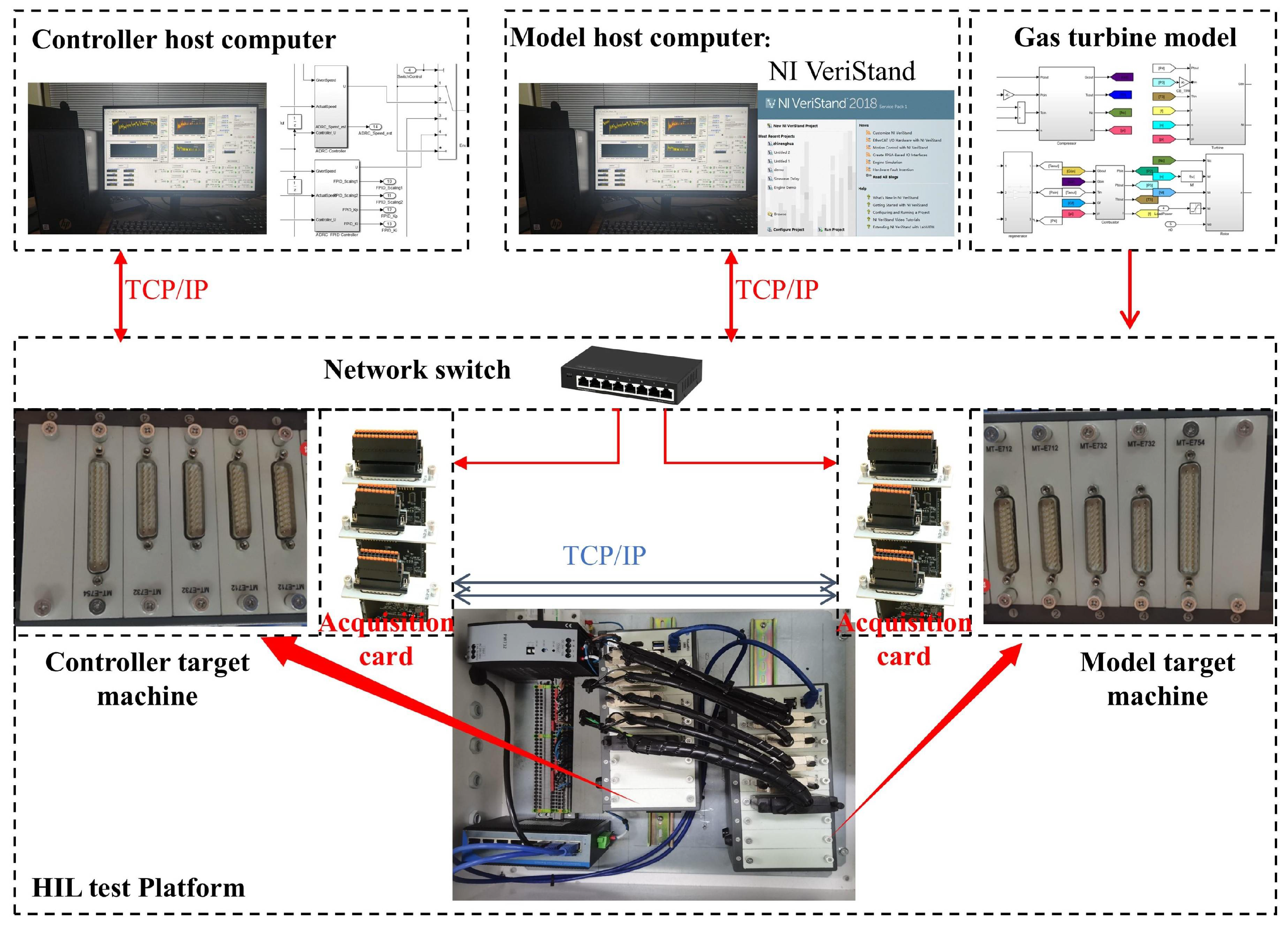
To validate the control performance of the NS_FADRC algorithm proposed in this paper, an HIL experimental platform was built, as shown in Figure 7. The platform mainly consists of four parts: the model host computer, the controller host computer, the model target machine, and the controller target machine. The hardware configuration is shown in

Table 2. Hardware configuration list of the HIL test Platform.

Device Name	Device Type	Device Model	Quantity	Performance Parameters
Model host computer	Computer	HP 288 Pro G6 Microtower PC	1	3.1 GHz i5-10500 CPU/8 GB
Controller host computer	Computer	HP 288 Pro G6 Microtower PC	1	3.1 GHz i5-10500 CPU/8 GB
Model target machine	RIO real-time device	RobustRIO U808	1	2.7 GHz Intel J4125 CPU/4 GB
	Acquisition card	MT-E732	2	$0 \mathrm{mA}\sim 25\mathrm{mA}$
		MT-E712	2	$\pm 25 \mathrm{mA}$
		MT-E754	1	24 V
Controller target machine	RIO real-time device	RobustRIO U808	1	2.7 GHz Intel J4125 CPU/4 GB
	Acquisition card	MT-E732	2	$0 \mathrm{mA}\sim 25 \mathrm{mA}$
		MT-E712	2	$\pm 25 \mathrm{mA}$
		MT-E754	1	24 V
Hardware boards	Network switch	T608F	1
	Power module	PW732	1

. Among these, the model host computer and the controller host computer are primarily used for simulation modeling and analysis, software-in-the-loop simulation, target machine code generation, compilation, linking, and downloading. During the HIL semi-physical testing process, the host computers are used to implement rich human–machine interaction functions. To meet the real-time requirements of the HIL semi-physical test environment, a real-time device based on the PharLap system is used as the target machine. The PharLap system is an industrial-grade real-time operating system with an interrupt response time of less than 1 microsecond, which meets the real-time requirements of the control system for HIL semi-physical testing. Additionally, the real-time device uses an 8-slot RobustRIO U808 chassis, which allows for easy expansion with its E-series and NI C-series boards. By adding A/D and D/A data acquisition cards, it is capable of signal conversion functionality.

To verify the advanced nature of the NS_FADRC algorithm, comparisons are made with the PID control algorithm, the fuzzy PID control algorithm (FPID), and the LADRC algorithm. The control object selected for this study is the micro gas turbine component-level simulation model developed by the author in reference [30]. Both the control system and the micro gas turbine simulation model are built on the Matlab 2021b platform, and Simulink Coder in MATLAB is used to automatically generate industrial control machine code that can run on the PharLap real-time operating system. All four control algorithms are based on the trial-and-error method for parameter tuning, with the tuned gain parameters shown in

Table 3. Summary table of gain parameters for four control algorithms.

Control Algorithms	Gain Parameters
PID	$K_P=3\times {10}^{-5}$$,K_I=1\times {10}^{-5}$
FPID	$K_{P0}=2.5\times {10}^{-5}$$,K_{I0}=1.0\times {10}^{-5}$$,k_1=2.0\times {10}^{-5}$$,k_2=8\times {10}^{-6}$
LADRC	$K_P=20$$,K_D=12$$,{\omega }_0=11$$,b_0=5\times {10}^5$
NS_FADRC	$K_{P0}=33$$,K_{D0}=25$$,{\omega }_0=12$$,b_0=5.2\times {10}^5$$,k_1=-20$$,k_2=-20$, $P=0.85$

. The trial-and-error method is an approach that relies on engineering experience to select the optimal control parameter combination by trying multiple parameter combinations. Based on engineering experience with gas turbine speed control, it is known that the differential term in the PID control introduces high-frequency oscillations, amplifying the effects of sensor measurement noise and disturbances on the control system, thus reducing system stability. Therefore, in this paper, the differential terms in the PID and FPID control algorithms are set to zero.

4.2. Speed Tracking Performance Test

The step response test is an important method for evaluating the dynamic response capability of the control system. At the same time, the variable-speed operation of the gas turbine is essentially a speed tracking process [31]. To verify the dynamic response capability of the proposed NS_FADRC algorithm and its control performance, the step-up acceleration tests from 50,800 r/min to 51,000 r/min and the step-down deceleration tests from 51,000 r/min to 50,800 r/min are conducted. The simulation environment for the model is based on ISO standard environmental conditions, and the load power is set to no load. The gain parameters for the PID, FPID, LADRC, and NS_FADRC algorithms are set according to those shown in Table 3. To more intuitively demonstrate the dynamic response capability of the proposed control algorithm, we use overshoot $\sigma$, rise time $t_r$, and settling time $t_s$ as evaluation criteria.

Figure 8 presents the speed step response results for the four controllers, with each controller’s response shown in different colored curves. The results indicate that, whether during the speed step-up acceleration or step-down deceleration process, all four control algorithms can effectively track the speed setpoint signal. Among them, the traditional PID control algorithm exhibits the largest overshoot and the longest settling time, while the NS_FADRC control algorithm demonstrates the smallest overshoot and no significant speed fluctuations. The dynamic performance indicators of the step response for all four control algorithms are detailed in

Table 4. Comparison of optimal indicator values for four control algorithms.

Control Algorithms	Step-Up Acceleration			Step-Down Deceleration
	$\mathit{\sigma }$/%	${\mathit{t}}_{\mathit{r}}$/s	${\mathit{t}}_{\mathit{s}}$/s	$\mathit{\sigma }$/%	${\mathit{t}}_{\mathit{r}}$/s	${\mathit{t}}_{\mathit{s}}$/s
PID	0.233	0.880	13.080	0.186	1.190	14.100
FPID	0.158	0.980	11.740	0.144	1.160	12.610
LADRC	0.026	1.100	3.360	0.0936	1.260	4.750
NS_FADRC	0.010	1.660	3.380	0.0341	1.420	4.080

.

Based on the analysis of the dynamic speed response performance of four control algorithms presented in Table 4, the findings are as follows:

(1) Overshoot: Overshoot intuitively reflects the degree of overshooting in the output characteristics of the system during a step response. The larger the overshoot is, the more intense the fluctuations in the system’s response are, indicating poorer stability. For micro gas turbine generator sets, excessive overshoot can deteriorate the combustion process, reduce structural strength, and degrade power quality. In both step-up and step-down processes, the overshoot of the PID control algorithm is the largest, at 0.233% and 0.186%, respectively. The overshoot of the LADRC algorithm is smaller than that of the FPID and PID algorithms. The NS_FADRC algorithm exhibits the smallest overshoot, with a value of 0.01% during acceleration, which is 95.7% lower than the PID control algorithm, and 0.0341% during deceleration, which is 81.7% lower than the PID control algorithm. Therefore, compared to the PID, FPID, and LADRC algorithms, NS_FADRC not only ensures the rapid tracking of speed targets but also maintains the smallest overshoot, making it more advantageous for the stable operation of the generator set.

(2) Rise time: The differences in rise time among the four control algorithms are relatively small. In the step-up acceleration process, the rise time for the PID control algorithm is 0.88 s, that for the FPID control algorithm it is 0.98 s, that for the LADRC algorithm it is 1.1 s, and that for the NS_FADRC algorithm it is 1.66 s. The rise time of NS_FADRC is longer than that of LADRC, the rise time of LADRC is longer than that of FPID, and the PID control algorithm has the shortest rise time. In the step-down deceleration process, the relationship between the rise times of the four algorithms follows the same trend as in the step-up acceleration process. Rise time characterizes the dynamic response speed of the control system: the shorter the time, the faster the response. However, for micro gas turbine generator sets, both too short and too long a rise time can have adverse effects on the system. A rise time that is too short may cause overshoot in the turbine speed and lead to excessive variations in fuel flow, affecting the quality of combustion. On the other hand, a rise time that is too long indicates a weaker dynamic response capability, potentially causing the control system to fail under large-scale transient changes. As shown in Figure 8, all four control algorithms achieve relatively short rise times, but the PID and FPID algorithms, due to their shorter rise times, result in larger overshoots in speed.

(3) Settling time: In the step acceleration phase, the PID control algorithm exhibits the longest settling time of 13.08 s, while the settling times of the FPID, NS_FADRC, and LADRC algorithms progressively decrease to 11.74 s, 3.38 s, and 3.36 s, respectively. In the step deceleration phase, the PID control algorithm again has the longest settling time of 14.1 s, followed by FPID with a settling time of 12.61 s. The LADRC algorithm achieves a settling time of 4.75 s, outperforming FPID, while NS_FADRC has the shortest settling time of 4.08 s. Notably, the settling times of the NS_FADRC and LADRC algorithms are significantly shorter than those of PID and FPID.

Based on the above analysis, it can be concluded that, in terms of speed tracking performance, the NS_FADRC algorithm outperforms the LADRC, FPID, and PID control algorithms. Both the NS_FADRC and LADRC algorithms adopt a design approach that integrates observer-based feedforward compensation with error feedback, resulting in significantly superior control performance compared to the PID-based architecture, which relies solely on passive feedback for error elimination.

4.3. Performance Testing Under Load Disturbance

In the gas turbine generator sets used in the MASS, external load disturbances are the most common source of disturbance. These are typically caused by factors such as the acceleration or deceleration of the vessel, or the connection or disconnection of high-power electrical equipment. These load disturbances directly impact the operating state of the gas turbine and represent a class of external disturbances that the control system must pay particular attention to. When an external load change occurs, the gas turbine’s most immediate response is speed fluctuations. To ensure power quality and the safety of the unit, the speed controller must be able to respond quickly and effectively to these load disturbances. Specifically, the controller adjusts the fuel flow to the gas turbine to rapidly eliminate speed fluctuations. Given that the characteristic parameters of the gas turbine vary with operating conditions, the designed control algorithm must exhibit excellent dynamic performance and robustness to effectively counteract the adverse effects of load disturbances under various operating conditions.

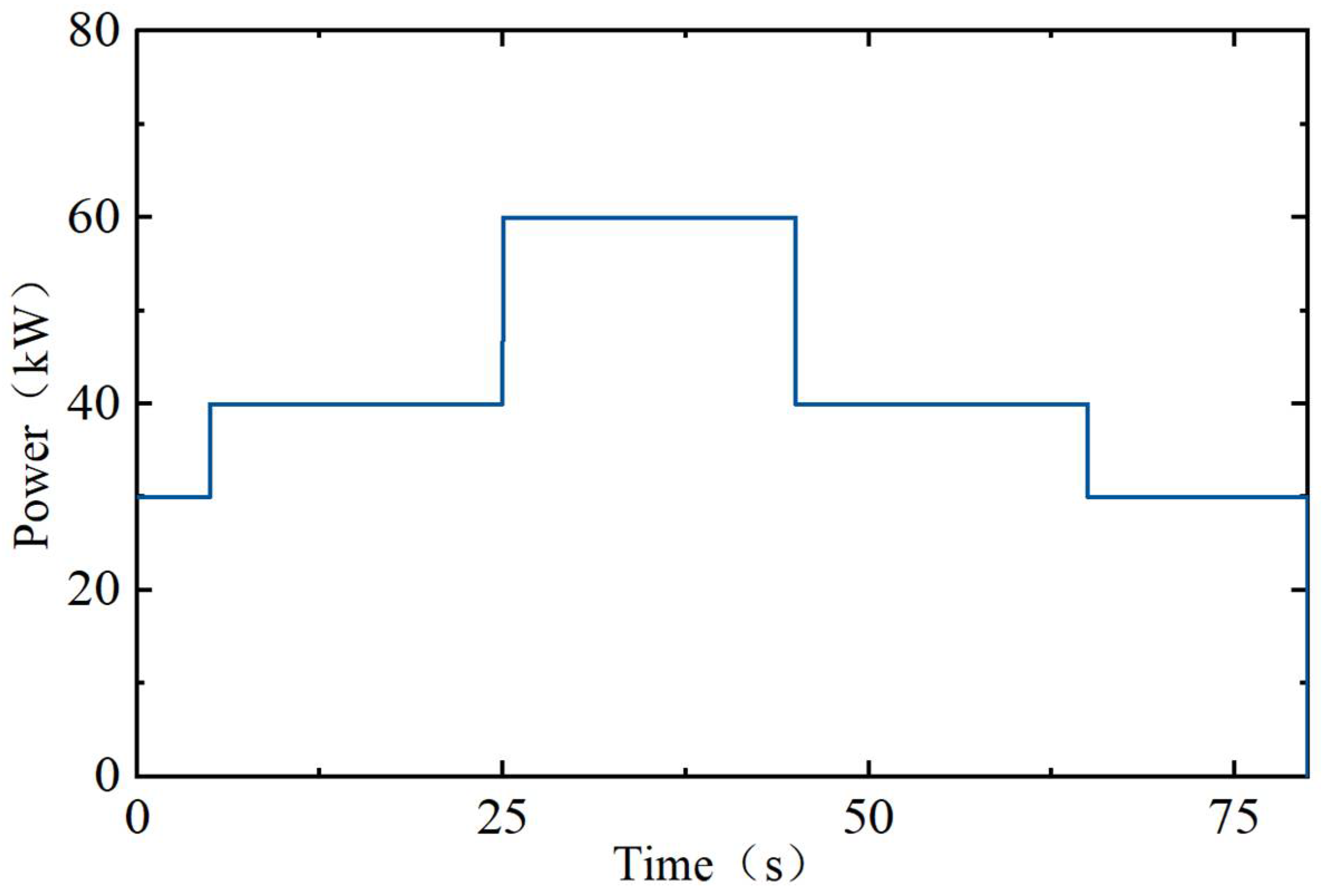
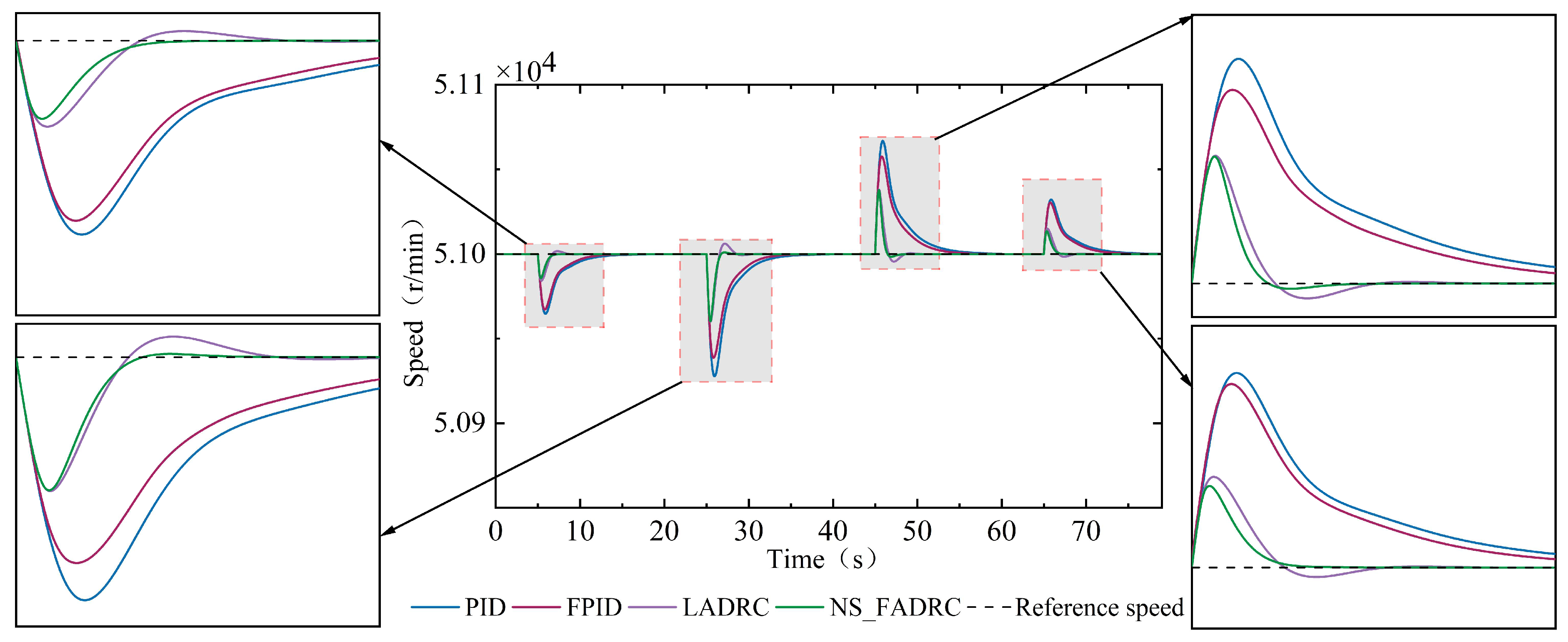
As shown in Figure 9, this study tests the control performance of the proposed speed control algorithms under four different operating conditions. For convenience, the four test operating conditions are labeled as A1, A2, A3, and A4, with their corresponding details shown in

Table 5. Four test operating condition parameters.

Operating Condition	Base Load (kW)	Load Change (kW)
A1	30	+10
A2	40	+20
A3	60	−20
A4	40	−10

. The speed response results of the four control algorithms under operating conditions A1, A2, A3, and A4 are presented in Figure 10. More detailed performance comparison results are provided in

Table 6. Performance indicators of four control algorithms under different load disturbances.

Performance Indicators	Operating Condition	PID	FPID	LADRC	NS_FADRC
Transient regulation rate (%)	A1	0.0692	0.0643	0.0307	0.0279
	A2	0.1418	0.1201	0.0782	0.0777
	A3	0.1311	0.1130	0.0746	0.0741
	A4	0.0631	0.0595	0.0294	0.0265
Settling time (s)	A1	9.81	8.05	3.26	1.85
	A2	11.46	9.38	4.56	2.66
	A3	12.75	10.60	3.37	2.69
	A4	10.78	8.97	3.28	1.81

The bolded entries in the table represent the optimal values.

.

From Figure 10, it can be seen that under the four test conditions (A1, A2, A3, and A4), all four control algorithms can effectively achieve stable speed control of the gas turbine. Furthermore, the speed deviation of the gas turbine is positively correlated with the magnitude of the load disturbance. However, among these four control algorithms, the conventional PID control algorithm exhibits the largest speed deviation, the longest settling time, and the poorest dynamic performance. Compared to the other three algorithms, the NS_FADRC algorithm has the smallest settling time and speed fluctuation amplitude under all four test conditions, indicating that this algorithm can effectively address the trade-off between the transient regulation rate and settling time, thereby achieving optimal dynamic performance. Similarly to the speed step tracking process, the performance of the NS_FADRC and LADRC algorithms significantly outperforms that of the FPID and PID control algorithms.

From Table 6, it can clearly be seen that under the A1 test condition, the transient regulation rate of the NS_FADRC algorithm is 0.0279%, which is only 0.41 times that of the PID control algorithm, 0.43 times that of the FPID control algorithm, and 0.91 times that of the LADRC algorithm. Meanwhile, the settling time of the NS_FADRC algorithm is 1.85 s, which is 7.96 s shorter than that of the PID control algorithm, 6.2 s shorter than that of the FPID control algorithm, and 1.41 s shorter than that of the LADRC algorithm. Under the A2, A3, and A4 conditions, the NS_FADRC algorithm performs better than the other three control algorithms in terms of both the transient regulation rate and settling time, with the improvement in settling time being especially significant for NS_FADRC.

4.4. Performance Testing Under Parameter Uncertainty

The application scenario of MASS is characterized by complex and variable working environments, extreme operating conditions, and unmanned operation. According to the external characteristics of gas turbines, the model parameters of the gas turbine can vary significantly with changes in load and environmental temperature. Model mismatch has become a challenging issue that is difficult to avoid in gas turbines. Therefore, a high-performance speed controller should exhibit robust performance to ensure that it can maintain excellent control effectiveness even when the gas turbine model parameters change. The previous Section has verified the performance of the NS_FADRC algorithm under varying load conditions. This Section will verify the speed control effect of this algorithm under different environmental temperatures.

To evaluate the performance of the speed control algorithm under different environmental temperatures, simulation tests were conducted at ambient temperatures of 5 °C and 20 °C. The test loads still used four typical non-design operating conditions, A1, A2, A3, and A4, with the control algorithm gain parameters taken from the data in Table 3.

First, with an ambient temperature T₀ = 5 °C, the speed response curves of the gas turbine under A1, A2, A3, and A4 conditions are shown in Figure 11. From Figure 11, it is clearly visible that compared to the traditional PID control algorithm, the FPID, LADRC, and NS_FADRC algorithms exhibit smaller speed deviations. In particular, the NS_FADRC algorithm stabilizes the speed at the rated value with the least speed deviation and the shortest time across all operating conditions. From

Table 7. The performance metrics of the four control algorithms at T₀ = 5 °C.

Performance Indicators	Operating Condition	PID	FPID	LADRC	NS_FADRC
Transient regulation rate (%)	A1	0.0647	0.0608	0.0303	0.0274
	A2	0.1325	0.1143	0.0751	0.0745
	A3	0.1343	0.1157	0.0762	0.0757
	A4	0.0654	0.0614	0.0306	0.0273
Settling time (s)	A1	11.01	9.20	3.29	2
	A2	12.77	10.60	3.47	1.83
	A3	12.84	10.68	3.43	2.78
	A4	11.07	9.27	3.24	1.93

The bolded entries in the table represent the optimal values.

, it can be directly observed that at T₀ = 5 °C, among the four control algorithms, the NS_FADRC algorithm achieves the smallest transient regulation rate and the shortest settling time under A1, A2, A3, and A4 conditions, indicating that it can still maintain the best dynamic response performance in low-temperature environments.

Next, we set the ambient temperature T₀ = 20 °C and conducted simulation tests on the four control algorithms under identical load conditions to evaluate their control performance at temperatures higher than the ISO standard environment. As shown in Figure 12, the PID control algorithm exhibits the largest speed deviation and significant fluctuations when the operating conditions change. In contrast, the FPID control algorithm shows smaller speed deviations than the PID algorithm, and the LADRC algorithm further reduces the speed deviation compared to the FPID. According to

Table 8. The performance metrics of the four control algorithms at T₀ = 20 °C.

Performance Indicators	Operating Condition	PID	FPID	LADRC	NS_FADRC
Transient regulation rate (%)	A1	0.0560	0.0534	0.0234	0.0218
	A2	0.1040	0.0912	0.0608	0.0605
	A3	0.1089	0.0948	0.0610	0.0604
	A4	0.0585	0.0554	0.0244	0.0226
Settling time (s)	A1	8.72	7.10	3.04	1.58
	A2	12.19	10.25	3.20	1.74
	A3	10.74	8.76	3.17	2.24
	A4	9.02	7.55	2.54	1.75

The bolded entries in the table represent the optimal values.

, the NS_FADRC algorithm demonstrates the smallest speed deviation and the shortest stabilization time compared to the other three algorithms. In conclusion, the NS_FADRC algorithm proposed in this paper maintains the best control performance even at temperatures above those of the ISO standard environment.

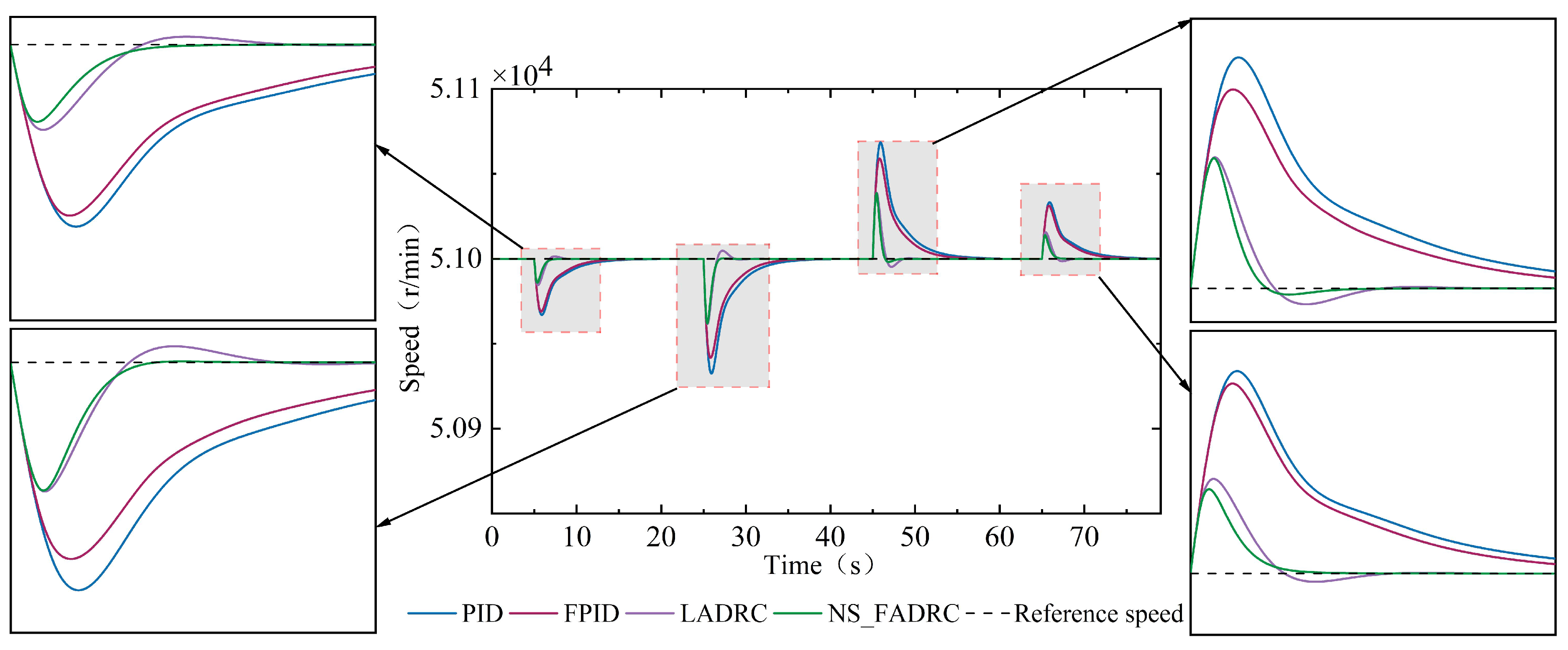
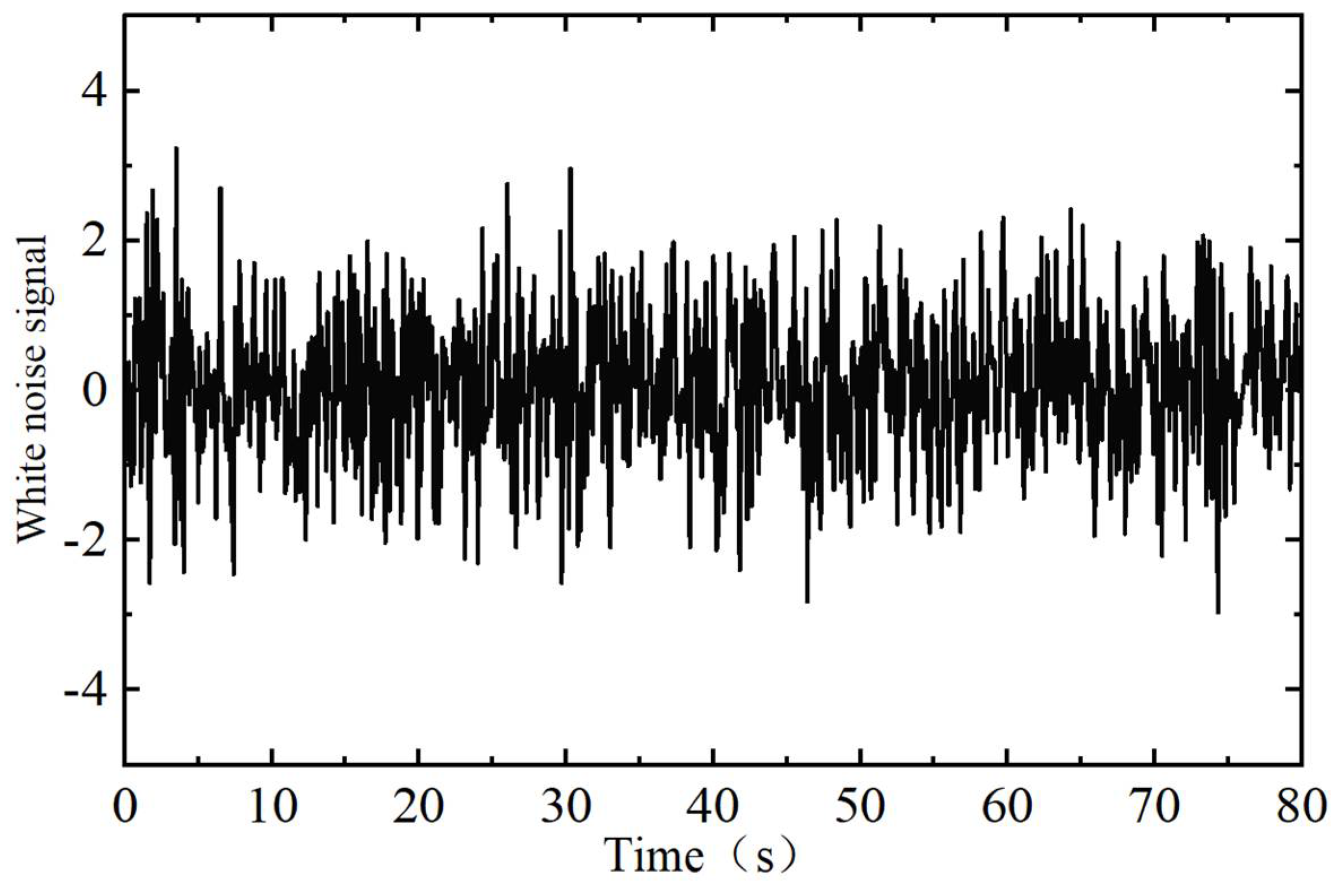
4.5. Performance Testing Under Measurement Noise Interference

In the actual operation of a gas turbine, the speed measurement signal is often affected by sensor measurement noise. To better simulate real-world scenarios, Gaussian white noise with a zero mean was added to the speed signal, as shown in Figure 13. The mathematical expression of the Gaussian white noise signal is $\vartheta (t)=A\cdot \kappa (t)$, where $\kappa (t)$ is a random variable that follows a Gaussian distribution with a mean of 0 and a variance of 1, and $A$ is a constant, which is taken as 2 in this paper. The test load conditions retain the labels of A1, A2, A3, and A4, with the gain parameters of the four control algorithms continuing to use the values from Table 3.

The gas turbine speed response results are shown in Figure 14. It can be observed that after the operating conditions change, the NS_FADRC algorithm achieves the smallest speed deviation and the shortest time to stabilize the speed at the rated value. In comparison, the speed deviation of the LADRC algorithm is similar to that of NS_FADRC, but it exhibits overshoot during the speed recovery phase, resulting in a longer stabilization time. The FPID control algorithm adjusts the parameters of the control algorithm using fuzzy logic, and its speed deviation and stabilization time are smaller than those of the PID control algorithm in all test conditions. Both LADRC and NS_FADRC utilize observers to estimate disturbances, significantly improving the disturbance rejection capability of the control algorithm, and their control performance in all four load disturbance conditions is far superior to that of the FPID and PID control algorithms.

Even in the presence of measurement noise in the speed signal, the NS_FADRC algorithm still demonstrates excellent dynamic response performance, indicating its strong robustness and adaptability to noise. This result further verifies the effectiveness and reliability of the NS_FADRC algorithm for practical gas turbine control.

5. Conclusions

This paper proposes a novel NS_FADRC speed control method for gas turbines, based on nonsmooth control theory and fuzzy control principles. Unlike conventional approaches, the proposed method does not require an accurate mathematical model of the gas turbine. Instead, it treats the unknown nonlinear dynamics and external disturbances of the system as perturbations, which are estimated and compensated for using the ESO. Furthermore, the traditional ESO is enhanced through nonsmooth control theory, enabling finite-time convergence and thereby improving its disturbance estimation capability. To overcome the limitations of traditional LSEF and NSEF, including poor adaptability to dynamic system changes, difficulty in tracking complex disturbances, and challenges in parameter tuning, the paper introduces fuzzy logic control. This leads to the design of a novel fuzzy adaptive control law that dynamically adjusts the parameters of the PD controller. The stability of the proposed control scheme is rigorously validated through Lyapunov-based stability analysis.

To demonstrate the effectiveness and superiority of the proposed control algorithm, an HIL semi-physical experimental platform is developed using automatic code generation technology. The NS_FADRC controller is compared against PID, FPID, and LADRC methods. Experimental results reveal that, under conditions such as speed step tracking, load disturbances, and the presence of parameter uncertainties and measurement noise, the NS_FADRC algorithm consistently outperforms the other methods in terms of control performance. In contrast to passive disturbance rejection approaches like PID and FPID, NS_FADRC actively estimates and compensates for disturbances, significantly enhancing the dynamic response and robustness of the gas turbine generator set on the MASS, thereby enhancing the maneuverability and reliability of the MASS. In addition, the research findings presented in this paper are also applicable to the control fields of industrial gas turbines and aircraft engines, demonstrating strong generalization ability and versatility.

References

1. Liu, Z.; Zhang, Y.; Yu, X.; Yuan, C. Unmanned surface vehicles: An overview of developments and challenges. Annu. Rev. Control 2016, 41, 71–93. [Google Scholar] [CrossRef]
2. Zhukov, V.; Butsanets, A.; Sherban, S. Design principles for onboard engineering diagnostics systems of unmanned maritime vessels. J. Phys. Conf. Ser. 2021, 2061, 12103. [Google Scholar] [CrossRef]
3. Palmieri, A.; Lanzarotto, D.; Cacciacarne, S.; Torre, I.; Bonfiglio, A. An innovative sliding mode load controller for gas turbine power generators: Design and experimental validation via real-time simulation. Energy 2021, 217, 119363. [Google Scholar] [CrossRef]
4. Zornek, T.; Monz, T.; Aigner, M. Performance analysis of the micro gas turbine Turbec T100 with a new FLOX-combustion system for low calorific fuels. Appl. Energy 2015, 159, 276–284. [Google Scholar]
5. Wu, D.; Wang, R. Combined cooling, heating and power: A review. Prog. Energy Combust. Sci. 2006, 32, 459–495. [Google Scholar]
6. Nascimento, M.A.R.; Rodrigues, L.O.; Santos EC d Gomes, E.E.B.; Dias, F.L.G.; Velásques, E.I.G.; Carrillo, R.A.M. Micro gas turbine engine: A review. Prog. Gas. Turbine Perform. 2013, 125, 1–14. [Google Scholar]
7. Oğuz, Y.; Üstün, S.V.; Yabanova, İ.; Yumurtaci, M.; Güney, İ. Adaptive neuro-fuzzy inference system to improve the power quality of a split shaft microturbine power generation system. J. Power Sources 2012, 197, 196–209. [Google Scholar] [CrossRef]
8. Rosini, A.; Palmieri, A.; Lanzarotto, D.; Procopio, R.; Bonfiglio, A. A model predictive control design for power generation heavy-duty gas turbines. Energies 2019, 12, 2182. [Google Scholar] [CrossRef]
9. Mohamed Iqbal, M.; Joseph Xavier, R. Fuzzy self-tuning PID controller for speedtronic governor controlled heavy duty gas turbine power plants. Electr. Power Compon. Syst. 2014, 42, 1485–1494. [Google Scholar]
10. Li, J.; Zhang, G.; Ying, Y.; Shi, W.; Bi, D. Marine three-shaft intercooled-cycle gas turbine engine transient thermodynamic simulation. Int. J. Perform. Eng. 2018, 14, 2289. [Google Scholar] [CrossRef]
11. Kim, D.-H. Neural Network Tuning of the 2-DOF PID Controller With a Combined 2-DOF Parameter For a Gas Turbine Generating Plant. Int. J. Fuzzy Log. Intell. Syst. 2001, 1, 95–103. [Google Scholar]
12. Wen, J.; Lu, J.; Zhang, S.; Liu, R.; Spataru, C.; Weng, Y.; Lv, X. Intelligent control for rapidity and security of all-electric ships gas turbine under complex mutation load using optimized neural network. Appl. Therm. Eng. 2024, 248, 123120. [Google Scholar] [CrossRef]
13. Tang, W.; Wang, L.; Gu, J.; Gu, Y. Single neural adaptive PID control for small UAV micro-turbojet engine. Sensors 2020, 20, 345. [Google Scholar] [CrossRef]
14. Jurado, F.; Acero, N.; Echarri, A. Enhancing the Electric System Stability using Predictive Control of Gas Turbines. In Proceedings of the 2006 Canadian Conference on Electrical and Computer Engineering, Ottawa, ON, Canada, 7–10 May 2006; pp. 438–441. [Google Scholar]
15. Saez, D.; Milla, F.; Vargas, L. Fuzzy predictive supervisory control based on genetic algorithms for gas turbines of combined cycle power plants. IEEE Trans. Energy Convers. 2007, 22, 689–696. [Google Scholar]
16. Haji, V.H.; Fekih, A.; Monje, C.A.; Asfestani, R.F. Adaptive model predictive control design for the speed and temperature control of a V94.2 gas turbine unit in a combined cycle power plant. Energy 2020, 207, 118259. [Google Scholar]
17. Ariffin, A.E.; Munro, N. Robust control analysis of a gas-turbine aeroengine. IEEE Trans. Control Syst. Technol. 1997, 5, 178–188. [Google Scholar] [CrossRef]
18. Gomma, H.W.; Owens, D.H. Robust control of gas generator in a 1.5 MW gas turbine engine. In Proceedings of the 1999 IEEE International Conference on Control Applications (Cat. No.99CH36328), Kohala Coast, HI, USA, 22–27 August 1999; pp. 634–639. [Google Scholar] [CrossRef]
19. Najimi, E.; Ramezani, M.H. Robust control of speed and temperature in a power plant gas turbine. ISA Trans. 2012, 51, 304–308. [Google Scholar]
20. Lin, P.; Du, X.; Shi, Y.; Sun, X.-M. Modeling and controller design of a micro gas turbine for power generation. ISA Trans. 2022, 124, 411–426. [Google Scholar] [CrossRef]
21. Gao, Z. Scaling and Bandwidth-Parameterization Based Controller Tuning. In Proceedings of the 2003 American Control Conference, Denver, CO, USA, 4–6 June 2003; pp. 1–9. [Google Scholar]
22. Wu, Z.; Li, D.; Liu, Y.; Chen, Y. Modified active disturbance rejection control based on gain scheduling for circulating fluidized bed units. J. Process Control 2024, 140, 103253. [Google Scholar] [CrossRef]
23. Wang, Y.; Fang, S.; Hu, J. Active disturbance rejection control based on deep reinforcement learning of PMSM for more electric aircraft. IEEE Trans. Power Electron. 2022, 38, 406–416. [Google Scholar]
24. Gong, Q.C.; Wu, Y.F. Auto Disturbance Rejection Control for Nonlinear Time-Delay Systems. Appl. Mech. Mater. 2013, 2218, 1547–1550. [Google Scholar] [CrossRef]
25. Bhat, S.P.; Bernstein, D.S. Finite-Time Stability of Continuous Autonomous Systems. SIAM J. Control Optim. 2006, 38, 751–766. [Google Scholar] [CrossRef]
26. Cui, S.; Zhao, T. Uncertain surface vessels tracking control based on linear active disturbance rejection control and finite time convergence. Ocean. Eng. 2024, 298, 117263. [Google Scholar] [CrossRef]
27. Li, S.; Wang, X. Finite-time consensus and collision avoidance control algorithms for multiple AUVs. Automatica 2013, 49, 3359–3367. [Google Scholar] [CrossRef]
28. Zhao, L.; Zhang, B.; Yang, H.; Wang, Y. Finite-time tracking control for pneumatic servo system via extended state observer. IET Control Theory Appl. 2017, 11, 2808–2816. [Google Scholar] [CrossRef]
29. Zhou, X.; Cui, Y.; Ma, Y. Fuzzy linear active disturbance rejection control of injection hybrid active power filter for medium and high voltage distribution network. IEEE Access 2021, 9, 8421–8432. [Google Scholar] [CrossRef]
30. Yang, R.; Liu, Y.; He, X.; Liu, Z. An Innovative Online Adaptive High-Efficiency Controller for Micro Gas Turbine: Design and Simulation Validation. J. Mar. Sci. Eng. 2024, 12, 2150. [Google Scholar] [CrossRef]
31. Duan, J.; Fan, S.; An, Q.; Sun, L.; Wang, G. A comparison of micro gas turbine operation modes for optimal efficiency based on a nonlinear model. Energy 2017, 134, 400–411. [Google Scholar] [CrossRef]
Figure 1. Relationship between the observation error input and the observed output under the NS_ESO and the LESO.
Jmse 13 00664 g001
Figure 2. Gas turbine speed response curve.
Jmse 13 00664 g002
Figure 3. Structure diagram of the FSEF.
Jmse 13 00664 g003
Figure 4. Fuzzy inference system input and output membership functions.
Jmse 13 00664 g004
Figure 5. The fuzzy rule map.
Jmse 13 00664 g005
Figure 6. The structure of NS_FADRC.
Jmse 13 00664 g006
Figure 7. Gas turbine HIL test platform.
Jmse 13 00664 g007
Figure 8. Gas turbine speed response curves.
Jmse 13 00664 g008
Figure 9. Gas turbine load power schedule curve.
Jmse 13 00664 g009
Figure 10. Speed response curves of the gas turbine under different operating conditions.
Jmse 13 00664 g010
Figure 11. The turbine speed response at T0 = 5 °C.
Jmse 13 00664 g011
Figure 12. The turbine speed response at T0 = 20 °C.
Jmse 13 00664 g012
Figure 13. Gaussian white noise signal.
Jmse 13 00664 g013
Figure 14. The gas turbine speed response curve under the influence of noise interference.
Jmse 13 00664 g014