Underwater Target Bearing Estimation Performance of Bottom-Mounted Extended Coprime Sparse Array

Abstract

Extended coprime sparse array (ECSA) has been widely used in signal processing, which realizes direction-of-arrival (DOA) estimation with fewer sensors. Accordingly, via spatial smoothing technique, an augmented sample covariance matrix was constructed. Then, the MUltiple SIgnal Classification (MUSIC) algorithm was applied in DOA estimation with higher-resolution ability, which is comparable to that of a uniform full array sharing the same aperture. As far as the application of underwater bottom-mounted horizontal ECSA, due to the property of multipath arrival, the estimated source bearing lies in between the true source bearing and the broadside direction of ECSA. Basically, for the problem of identifying a specific target in the presence of interferers, with regard to both bearing resolution performance and corresponding estimation accuracy, a relationship with the true source positions was established. It was proven that the MUSIC algorithm suffers from an intrinsic error, which is driven by energy-dominant modes in the waveguide. Based on the multimode phenomenon, this paper reveals the influence of source position, especially the angular arrangement. Additionally, on the premise of successful target resolution, reference sound speed substitution was carried out to achieve improved bearing estimation accuracy. The results are herein demonstrated with both numerical simulation and experimental data.

1. Introduction

Multiple current approaches to array signal processing have been introduced by sparse linear arrays. One of the typical categories is namely the coprime sparse array (CSA), which is constructed by a combination of two uniform linear arrays (ULAs) with different interelement spacings. Thus, the attractive capability of providing enhanced degrees of freedom is achieved [1,2,3,4]. Yang et al. [5] illustrated that, using coherent product processing, the coprime array is able to yield an array gain equivalent to that of the full array, with far fewer array sensors required. Qin et al. [6] proposed the generalization of the coprime array concept, which comprises two operations of coprime array with compressed inter-element spacing (CACIS) and coprime array with displaced subarrays (CADiS). However, the peak of the sidelobe is considerably higher. By adding extra sensors, Adhikari et al. [7,8] represented the extended coprime structure to guarantee that the peak sidelobe height of the coprime array is less than that of the full array. Furthermore, Moghadam et al. [9] introduced the optimization problem of coprime structure configuration. Practically, Chen et al. [10,11] made use of an underwater coprime vector sensor array to estimate co-frequency sources, and the spatial resolution and the left-right ambiguity rejection capability were both improved by the proposed method. Typically, in consideration of sparse array design under certain constraints, optimization algorithms such as the global enhancement whale algorithm were deemed suitable for use [12].

In order to estimate the DOA of a moving source in an underwater environment with a low signal-to-noise ratio (SNR), Dong et al. developed a framework of particle filter with sequential importance resampling [13]. In the presence of impulsive noise, Pan et al. [14] proposed an enhanced fractional low-order method to improve the resolution, accuracy, and degrees of freedom in DOA estimation. And they also extracted the multiple-measurement matrix from the specific columns of the covariance matrix directly. As a result, the time-delay estimation was obtained by MUSIC algorithm without additional decoherence preprocessing [15]. Based on deep learning, Su et al. established an algorithm for co-prime array interpolation, which employs the covariance matrix of the interpolated virtual array to construct a self-supervision loss function based on the Hermitian semi-definite Toeplitz condition [16].

Typically, by exploiting the coprime structure, an augmented sample covariance matrix can be constructed by the use of techniques such as spatial smoothing (SS). Then, the MUltiple SIgnal Classification (MUSIC) algorithm can be utilized in the difference-coarray domain. As a result, it was found feasible to separate the signal subspace and the noise subspace based on eigenvalues of the spatially smoothed matrix [17,18,19]. Wang et al. [20,21] derived the asymptotic mean square error (MSE) expression for an SS-based MUSIC algorithm, which converges to a positive value instead of zero when the signal-to-noise ratio (SNR) goes to infinity. Moreover, the proposed MSE expression was proven valid when the number of sources exceeds the number of sensors. Furthermore, the underwater acoustical environment is a complex and dynamic three-dimensional acoustic medium, with its properties significantly influencing underwater acoustic propagation. On one hand, in the water column, refraction could be caused by vertical stratification, which is created by density, salinity, and pressure. On the other hand, internal waves could also generate periodic sound speed perturbations, which leads to spatiotemporal acoustic field variations, such as signal scintillation and path deviations [22,23,24]. As for a bottom-mounted horizontal linear array (HLA) in the underwater scenario, those methods are all based on plane-wave hypothesis. By conventionally weighting in beamforming, bearing estimation is deviated due to the multipath phenomenon [25,26,27,28,29]. Based on either the MUSIC algorithm or coprime structure, the underwater acoustic propagation mechanism has not been taken into consideration by the existing source resolution methods.

In this study, the concept of the coprime array was integrated into a bottom-mounted HLA. Particularly, the considered typical shallow-water scenario involved a downward-refracting sound speed profile (SSP) with a negative thermocline. In addition, for the problem of target bearing estimation in the presence of a near-surface interferer, numerical analysis was carried out. According to the assumed condition, in the water column, direction-of-arrival (DOA) estimation is considerably related to the spatial position of both the target and the interferer. Correspondingly, experimental results revealed the phenomenon of multipath arrival and verified the performance variation in target bearing estimation.

The rest of the paper is organized as follows. In Section 2, the coprime array configuration used in this paper, SS-based MUSIC algorithm, and deviating feature in underwater bearing estimation are briefly introduced. Subsequently, Section 3 presents the typical simulation results. Based on a normal-mode model, variation in bearing estimation performance is numerically analyzed in different conditions of source position. Then, Section 4 presents the target bearing estimation results for experimental data collected in the South China Sea, and conclusions are provided in Section 5.

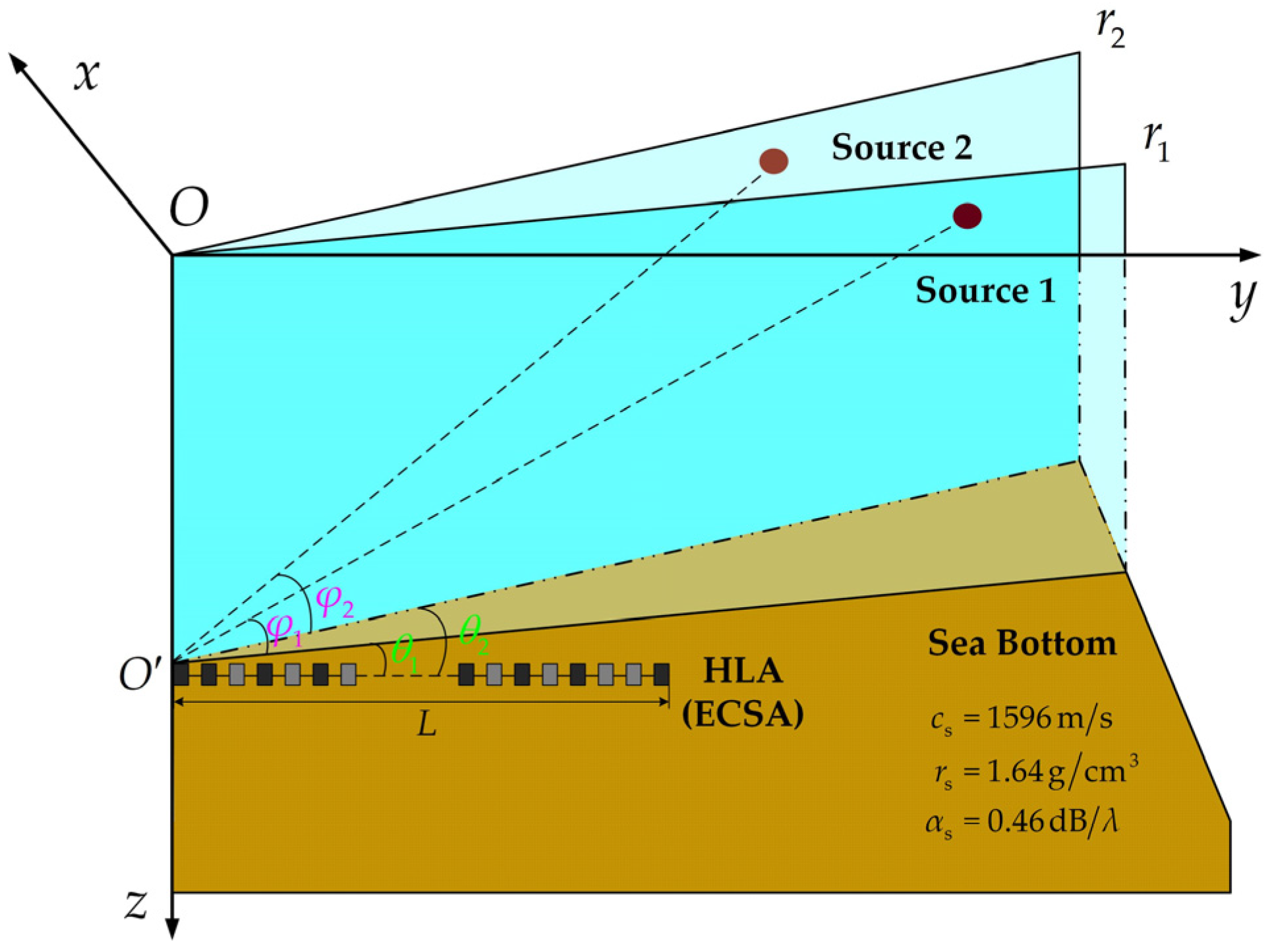
2. ECSA in Underwater Waveguide

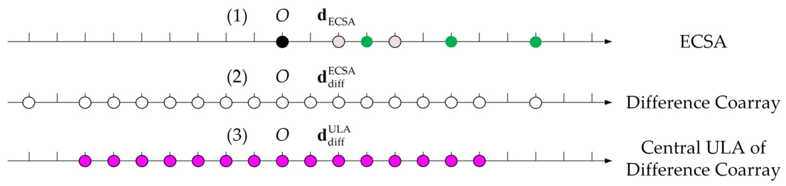
2.1. Configuration of ECSA and Spatial Smoothing Technique

Commonly, CSA takes advantage of two interleaved subarrays consisting of A and B sensors, where A and B are coprime integers. Thus, the grating lobes of the two subarrays appear at different angles, which are suppressed by superposition; then, satisfactory resolution is provided. In this paper, an extended CSA (ECSA) is considered, which makes use of 2A samples from the first subarray and B samples from the second [2], for instance, given that the coprime integer pair is (A, B) = (2, 3), as shown in Figure 1. For subarray 1, the uniform spacing of the 2A sensors is $B\lambda /2$, where λ represents wavelength of the signal. For subarray 2, the uniform spacing of the B sensors is $A\lambda /2$. Since the first sensor is shared by both subarrays, the total number of sensors in the ECSA is $2A+B-1$, resulting in the following configuration:

$$\begin{array}{c}{d}_{\mathrm{ECSA}}=\left\{\left[0,B,\dots ,\left(2A-1\right)B\right]\cup \left[0,A,\dots ,\left(B-1\right)A\right]\right\}\left(\lambda /2\right)\\ =\left[0,2,3,4,6,9\right]\left(\lambda /2\right),\hspace{1em}\hspace{1em}\hspace{1em}\hspace{1em}\hspace{1em}\hspace{1em}\hspace{1em}\hspace{1em} \end{array}$$

(1)

which is made up of six sensors. By denoting the unit sensor spacing as $d_0$ (ideally equal to $\lambda /2$), then the configuration of ECSA is expressed as $d_{\mathrm{ECSA}}=\left[d_1,d_2,\dots ,d_N\right]$. In the presence of P narrow-band sources from directions ${\theta }_p$ with powers ${\sigma }_p^2$ ($p=1,2,\dots ,P$), the received signal vectors can be written as follows:

$${\mathit{y}}_{d_{\mathrm{ECSA}}}={\mathit{A}}_{d_{\mathrm{ECSA}}}{\mathit{x}}_{d_{\mathrm{ECSA}}}+{\mathit{n}}_{d_{\mathrm{ECSA}}},$$

(2)

where ${\mathit{A}}_{d_{\mathrm{ECSA}}}=\left[{\mathit{a}}_{d_{\mathrm{ECSA}}}\left({\theta }_1\right),{\mathit{a}}_{d_{\mathrm{ECSA}}}\left({\theta }_2\right),\dots ,{\mathit{a}}_{d_{\mathrm{ECSA}}}\left({\theta }_P\right)\right]$ denotes the array steering matrix; ${\mathit{x}}_{d_{\mathrm{ECSA}}}$ and ${\mathit{n}}_{d_{\mathrm{ECSA}}}$ represent the signal vector and the additive white Gaussian noise, respectively. Then, assuming that the sources are distinct and uncorrelated, the sample covariance matrix can be represented by the following:

$${\mathit{R}}_{d_{\mathrm{ECSA}}}=E\left[{\mathit{y}}_{d_{\mathrm{ECSA}}}{\mathit{y}}_{d_{\mathrm{ECSA}}}^{\mathrm{H}}\right]={\displaystyle \sum _{p=1}^P{\sigma }_p^2{\mathit{a}}_{d_{\mathrm{ECSA}}}\left({\theta }_p\right){\mathit{a}}_{d_{\mathrm{ECSA}}}^{\mathrm{H}}\left({\theta }_p\right)}+{\sigma }_n^2\mathit{I},$$

(3)

where ^H denotes the conjugate transpose, and I represents an identity matrix. Equation (3) also implies that the additive noise is uncorrelated with the sources and has a steady power of ${\sigma }_n^2$. On the basis of $d_{\mathrm{ECSA}}$, elements of $\exp \left[j2\pi \left(n_1-n_2\right)\right]$ (for $n_1,n_2\in d_{\mathrm{ECSA}}$) are contained in ${\mathit{R}}_{d_{\mathrm{ECSA}}}$, which indicates dependency on the differences of sensor locations in the ECSA. Consequently, the corresponding difference coarray could be built as $d_{\mathrm{diff}}^{\mathrm{ECSA}}=\left\{\left.n_1-n_2\right|n_1,n_2\in d_{\mathrm{ECSA}}\right\}$. For conciseness, $d_{\mathrm{diff}}^{\mathrm{ECSA}}$ is prearranged in ascending order, which implies that the first and the last element of ${\mathit{y}}_{d_{\mathrm{diff}}^{\mathrm{ECSA}}}$ correspond to $\min \left[d_{\mathrm{diff}}^{\mathrm{ECSA}}\right]$ and $\max \left[d_{\mathrm{diff}}^{\mathrm{ECSA}}\right]$, respectively. When the ECSA is designed appropriately, note that the difference coarray principally contains a ULA part that is centered at the origin. Then, the virtual ULA containing 15 sensors can be denoted by $d_{\mathrm{diff}}^{\mathrm{ULA}}$, which is also illustrated in Figure 1.

According to the relationship between $d_{\mathrm{diff}}^{\mathrm{ECSA}}$ and $d_{\mathrm{diff}}^{\mathrm{ULA}}$, the signal over $d_{\mathrm{diff}}^{\mathrm{ULA}}$ is then constructed, making it plausible to rewrite Equation (2) as follows:

$${\mathit{y}}_{d_{\mathrm{diff}}^{\mathrm{ULA}}}={\displaystyle \sum _{p=1}^P{\sigma }_p^2{\mathit{a}}_{d_{\mathrm{diff}}^{\mathrm{ULA}}}\left({\theta }_p\right)}+{\sigma }_n^2{\mathit{e}}_{d_{\mathrm{diff}}^{\mathrm{ULA}}},$$

(4)

where ${〈{\mathit{e}}_{d_{\mathrm{diff}}^{\mathrm{ULA}}}〉}_u={\delta }_{u,0}$ for $u\in d_{\mathrm{diff}}^{\mathrm{ULA}}$, and the bracket notation conveys the value at auxiliary location u in the sequence of $d_{\mathrm{diff}}^{\mathrm{ULA}}$. Moreover, in order to apply the MUSIC algorithm, a spatial smoothed matrix ${\mathit{R}}_{\mathrm{SS}}$ is supposed to be established as follows:

$${\mathit{R}}_{\mathrm{SS}}={\displaystyle \frac{1}{V}}{\displaystyle \sum _{v=0}^{V-1}{\mathit{J}}_v{\mathit{y}}_{d_{\mathrm{diff}}^{\mathrm{ULA}}}{\mathit{y}}_{d_{\mathrm{diff}}^{\mathrm{ULA}}}^{\mathrm{H}}{\mathit{J}}_v^{\mathrm{H}}}.$$

(5)

The selection matrix ${\mathit{J}}_v$ is defined as follows:

$${\mathit{J}}_v=\left[\begin{array}{ccc}{\mathit{O}}_{V\times \left(V-1-v\right)}& {\mathit{I}}_{V\times V}& {\mathit{O}}_{V\times v}\end{array}\right]\in {\left\{0,1\right\}}^{V\times \left(2V-1\right)},$$

(6)

where O is the notation of null matrix, and $V=\left(\left|d_{\mathrm{diff}}^{\mathrm{ULA}}\right|+1\right)/2$. $\left|\cdot \right|$ is used to represent the cardinality [10].

In practical application, for the ECSA, the measured vector is expressed as ${\tilde{\mathit{y}}}_{d_{\mathrm{ECSA}}}$, where the tilde character is used to indicate measured quantity. Then, the estimated covariance matrix ${\tilde{\mathit{R}}}_{d_{\mathrm{ECSA}}}$ can be obtained over limited available snapshots, through which ${\tilde{\mathit{y}}}_{d_{\mathrm{diff}}^{\mathrm{ECSA}}}$ is determined:

$${〈{\tilde{\mathit{y}}}_{d_{\mathrm{diff}}^{\mathrm{ECSA}}}〉}_u={\displaystyle \frac{1}{\left|U\left(u\right)\right|}}{\displaystyle \sum _{\left(n_1,n_2\right)\in U\left(u\right)}{〈{\tilde{\mathit{R}}}_{d_{\mathrm{ECSA}}}〉}_{n_1,n_2}},u\in d_{\mathrm{diff}}^{\mathrm{ECSA}}.$$

(7)

The set $U\left(u\right)$ assembles all pairs of $\left(n_1,n_2\right)$, which produce the index of difference coarray:

$$U\left(u\right)=\left\{\left.\left(n_1,n_2\right)\in d_{\mathrm{ECSA}}^{\mathrm{H}}{d}_{\mathrm{ECSA}}\right|n_1-n_2=u\in d_{\mathrm{diff}}^{\mathrm{ECSA}}\right\}.$$

(8)

Similarly, the measurement vector over $d_{\mathrm{diff}}^{\mathrm{ULA}}$ can be constructed as follows:

$${〈{\tilde{\mathit{y}}}_{d_{\mathrm{diff}}^{\mathrm{ULA}}}〉}_u={\displaystyle \frac{1}{\left|U\left(u\right)\right|}}{\displaystyle \sum _{\left(n_1,n_2\right)\in U\left(u\right)}{〈{\tilde{\mathit{R}}}_{d_{\mathrm{ECSA}}}〉}_{n_1,n_2}},u\in d_{\mathrm{diff}}^{\mathrm{ULA}}.$$

(9)

On this basis, the measured spatial smoothed matrix is computed according to Equation (5); then, MUSIC algorithm can be applied.

2.2. Bearing Deviation of Underwater HLA

In an underwater waveguide, the directional response of a bottom-mounted HLA highly depends on the underwater acoustic propagation characteristics. Depending on the mode theory, pressure impinging on each array sensor can be expressed as a sum of M propagating normal modes [30]:

$$p\left(\omega ;r_n,z_{\mathrm{r}}\right)={\displaystyle \frac{j}{\rho \left(z_{\mathrm{s}}\right)\sqrt{8\pi r_n}}}{e}^{-j{\displaystyle \frac{\pi }{4}}}{\displaystyle \sum _{m=1}^M{\mathsf{\Psi }}_m\left(z_{\mathrm{s}}\right){\mathsf{\Psi }}_m\left(z_{\mathrm{r}}\right)\frac{e^{j{k}_m{r}_n}}{\sqrt{k_m}}},n=1,2,\dots N,$$

(10)

where ω is the angular frequency, $z_{\mathrm{r}}$ is the receiver depth, and $\rho \left(z_{\mathrm{s}}\right)$ represents the density of water column at the source depth $z_{\mathrm{s}}$. $r_n$ represents the horizontal ranges from the source to the nth sensor; $k_m$ and ${\mathsf{\Psi }}_m$ are the horizontal wavenumber and the eigenfunction of the mth mode, respectively. Furthermore, HLA has an exclusive feature that the end-fire beam is different from the broadside beam, which is caused by beam spreading of a non-broadside source. From the aspect of mode theory, the acoustic field is a coherent summation of normal modes, which can be regarded as a superposition of plane waves with discrete angles and corresponding amplitude shading. Given that the true bearing of underwater source is ${\theta }_{\mathrm{T}}$ (measured from the end-fire direction), then the arrival angle of the mth mode ${\theta }_m$ can be obtained as follows:

$$\cos {\theta }_m=\cos {\theta }_{\mathrm{T}}\cos {\phi }_m=k_m\cos {\theta }_{\mathrm{T}}/k_{\mathrm{ref}},$$

(11)

where ${\phi }_m$ represents the vertical arrival angle of the mth mode, and $k_{\mathrm{ref}}=\omega /c_{\mathrm{ref}}$ is the reference wavenumber at the receiving depth of HLA. Since $\left|\cos {\phi }_m\right|\le 1$, the estimated bearing for each mode is supposed to be deviated to the broadside. Hence, the bearing estimation result is determined by both ${\theta }_{\mathrm{T}}$ and ${\phi }_m$.

By establishing a coordinate system along the HLA, signal bearings and vertical arrival angles are geometrically illustrated in Figure 2, which indicates that the DOA deviation varies depending on the source position. Incidentally, the following analysis of ECSA is rooted in the uniform HLA, which is actually deployed in practice.

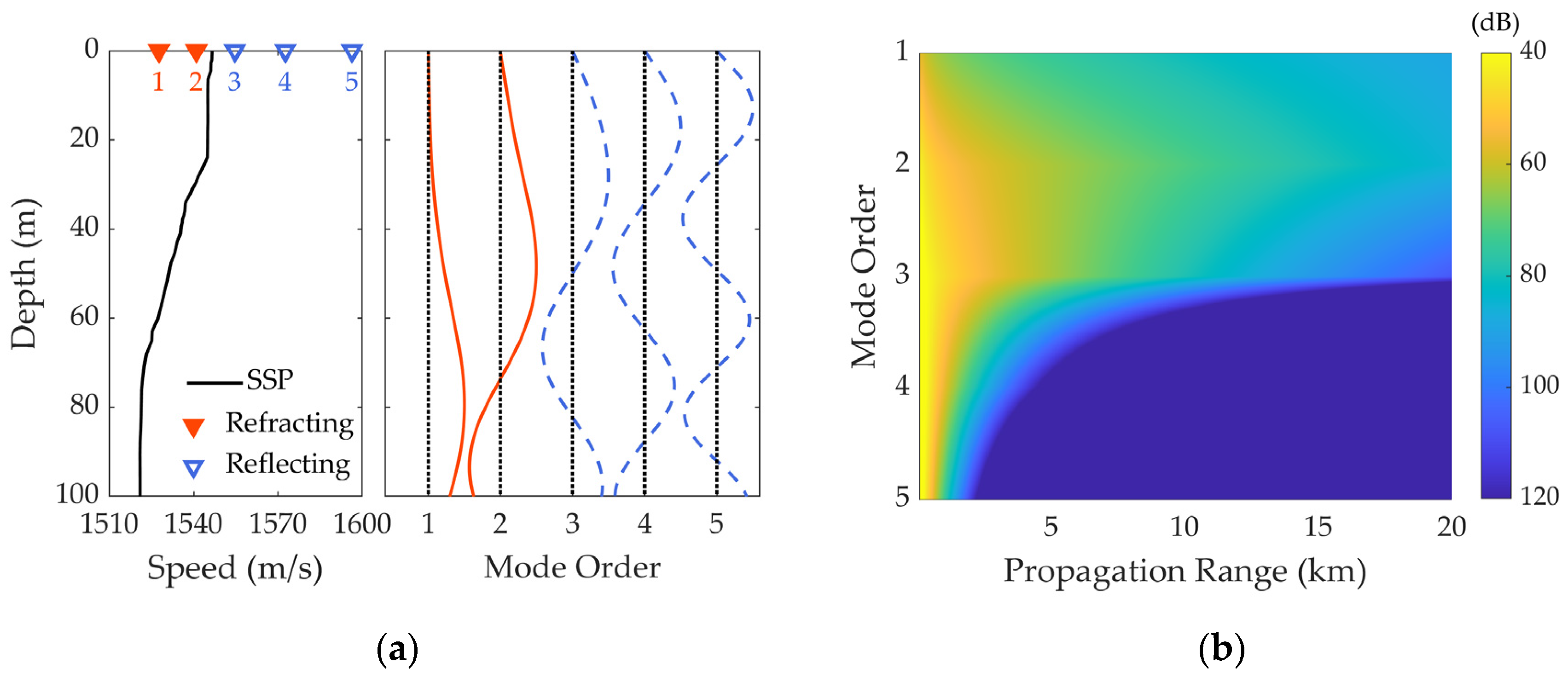
2.3. Energy Trapping of Refracting Modes

It is well known that the phase velocity represents the horizontal velocity of a particular phase in the plane-wave representation of a propagating mode, which is defined as $v_m=\omega /k_m$ ($m=1,2,\dots ,M$). In a shallow-water acoustic field, the phase velocity is always larger than the speed of sound in the water column, although the gap between them gets smaller as frequency increases [31]. When approaching the cutoff frequency, the plane waves interfere to produce a mode propagating nearly vertically, whereas the modal plane waves in the high-frequency limit propagate close to the horizontal. As a result, for steep propagation angles, the phase velocity approaches infinity, while the horizontal propagation yields a phase velocity equal to the speed of sound.

On the basis of Snell’s law, the critical grazing angle is found to be ${\theta }_{\mathrm{critical}}=\arccos \left(c_1/c_2\right)$, where $c_1$ and $c_2$ represent the sound speed in the upper and lower media, respectively [32]. For grazing angles smaller than ${\theta }_{\mathrm{critical}}$, perfect reflection occurs at the interface, accompanied with an angle-dependent phase shift. In the case of shallow-water acoustic propagation, the media primarily refer to the water column and the sea bottom. In consequence, for a propagating mode, the critical angle exists only when the phase velocity is higher than the sound speed in the sediment. It is indicated that the acoustic energy predominantly comprises effective modes with elevation angles less than the critical angle, which leads to low reflection loss.

Typically, for an environment with a downward-refracting SSP structure, modes whose phase velocity satisfies $c_{\max }<v_m<c_{\mathrm{s}}$ are defined as reflecting modes, where $c_{\max }$ and $c_{\mathrm{s}}$ represent the maximum sound speed in the water column and sound speed in the sediment, respectively. The reflecting modes interact with the surface and bottom boundary of the waveguide alternately. While $v_m<c_{\max }$, the corresponding modes are defined as refracting modes, and the energy carried by them would be trapped below the upper boundary of the thermocline. These two types of modes are accompanied by a relatively small grazing angle so that they do not penetrate the sea bottom. Thus, with most of the energy retained, the maximum estimated bearing driven by these modes can be derived by ${\theta }_{\max }=\arccos \left(c_{\mathrm{ref}}\cos \theta /c_{\mathrm{s}}\right)$, where $c_{\mathrm{ref}}$ is considered as the measured sound speed $c_{\mathrm{r}}$ at the depth of ECSA, namely the minimum sound speed in the water column. To put it another way, as propagation range increases, due to repeated interaction with the sea bottom, higher-order modes ($m>5$ herein) suffer remarkable loss. As a result, the energy of underwater targets is mainly contained in the low-order modes. Consequently, the estimated bearing ought to range between ${\theta }_{\mathrm{T}}$ and ${\theta }_{\max }$ when the propagation range is large enough, and it converges to the arrival angle of energy-dominant modes.

As illustrated in the left panel of Figure 3a, the experimentally measured SSP consists of a negative thermocline (ranging from 23.8 m to 87.7 m), which implies that $c_{\mathrm{r}}$= 1520.9 m/s is the minimum sound speed in the water column; then, the acoustic energy would accumulate around the sea bottom. For a 120 Hz narrow-band signal, the first five depth-dependent normal mode functions calculated via the KRAKEN model are depicted in the right panel of Figure 3a, where refracting modes and reflecting modes are differentiated by line style [33]. Overall, the mode functions oscillate sinusoidally with respect to depth, and the variation period gets shorter when the mode order or the water depth increases. And it is notable that as the vertical wavenumber becomes imaginary, mode function curves turn to decaying evanescently above the thermocline. The very turning depth corresponds to the position where SSP exceeds the phase velocity, which gets shallower with the mode order. In particular, for the mode whose phase velocity does not intersect with the SSP, the turning depth goes beyond the sea surface. Moreover, if the source or the receiver is located at a node of the mth mode function, then the mth mode does not make any contribution to the received signal.

Above all, on account of the downward-refracting environment, the amplitude of each mode function is nonzero at the bottom boundary. Hence, by fixing the receiving depth at the sea bottom, namely around 100 m, the excitation level of each mode varies according to the source depth. Typically, refracting modes (lower-order modes, m = 1, 2 herein) can be barely excited by near-surface source, which is shallower than the upper boundary of the thermocline [34,35,36].

Correspondingly, the transmission loss of the first five modes is displayed in Figure 3b. It is indicated that under the same condition of excitation level, the energy of higher-order reflecting modes attenuates rapidly. In other words, only lower-order refracting modes are capable of propagating over a long distance, which makes the feature of mode trapping more outstanding with increasing propagation range. Therefore, the two types of modes can be differentiated by modal energy distribution, which is then associated with the source position. In addition, based on the relationship between the true source bearing and signal-arrival angles shown in Equation (11), higher-order modes suffer much severer deviation, and the modal arrival angles are bound to appear in a wider angular range.

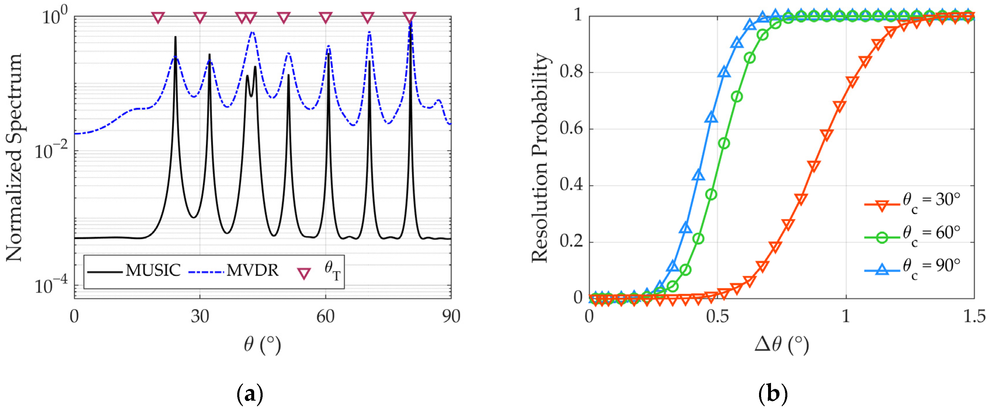
2.4. Performance of the MUSIC Estimator

As far as the accuracy of DOA estimation is concerned, the averaged root mean square error (RMSE) can be used for the purpose of quantification. The following considers that the estimated bearing is $\widehat{\theta }$:

$$\mathrm{RMSE}=\sqrt{{\displaystyle \frac{{\displaystyle \sum _{p=1}^P{\displaystyle \sum _{q=1}^Q{\left(\widehat{\theta }\left(p,q\right)-{\theta }_{\mathrm{T}}\left(p,q\right)\right)}^2}}}{PQ}}},$$

(12)

where P and Q represent the number of sources and Monte Carlo trials, respectively. Besides the DOA estimation error, if two adjacent sources are able to be identified by the MUSIC algorithm, they are defined as a resolvable pair in the angular domain [13]. Then, in this paper, the performance of the MUSIC estimator is evaluated under a premise of resolvability. Practically, the problem of source resolution can be addressed as a binary hypothesis test, through which resolvability ($H_0$) and irresolvability ($H_1$) are recognized by the following criterion:

$$\left\{\begin{array}{c}{H}_0:\widehat{\theta }\left(i\right)\in \left[{\theta }_{\mathrm{T}}\left(i\right)-\Delta \theta /2,{\theta }_{\max }\left(i\right)+\Delta \theta /2\right]\\ H_1:\widehat{\theta }\left(i\right)\notin \left[{\theta }_{\mathrm{T}}\left(i\right)-\Delta \theta /2,{\theta }_{\max }\left(i\right)+\Delta \theta /2\right]\end{array}\right., i=1,2.$$

(13)

In other words, resolvability is achieved when both of these estimated DOAs satisfy $\widehat{\theta }\in \left[{\theta }_{\mathrm{T}}-\Delta \theta /2,{\theta }_{\max }+\Delta \theta /2\right]$.

In consideration of both the port–starboard ambiguity and bearing deviation symmetry about the broadside direction, the source bearing is concentratedly studied ranging from 0° to 90°. By adopting the ECSA configuration, the comparison between the MUSIC and minimum variance distortionless response (MVDR) algorithms is shown in Figure 4a given that there are eight sources distributed in the underwater space, and the true bearings of them are [20, 30, 40, 42, 50, 60, 70, 80]°, respectively. As can be seen, compared with the poorer capacity of MVDR, all the DOAs are clearly identified in the spatial spectrum of ECSA, where all of the eight distinguishable peaks can be observed, and the mean estimation error of the sources is 1.43°. It is also notable that for sources deviating from the broadside direction, the range of mode arrival angles is widened according to the multimode phenomenon, and the phase variation rate of the steering vector gets slower. As a result, the corresponding source distinguishability is reduced.

Attributed to the use of the spatial smoothing technique, the aperture of the virtual ULA originated from the ECSA is 39$d_0$. In addition, given that the angular separation between the sources is $\Delta \theta$, and the central angle is denoted by ${\theta }_{\mathrm{c}}$, the true bearings of the two sources are ${\theta }_1={\theta }_{\mathrm{c}}-\Delta \theta /2$ and ${\theta }_2={\theta }_{\mathrm{c}}+\Delta \theta /2$, respectively. Subsequently, under different angular separations, Figure 4b displays the resolution probability derived by the root-MUSIC algorithm, where 1000 independent trials are involved. By the decision metric described in Equation (13), the resolution probability of both arrays drops to zero as the angular separation of the sources gets smaller, and the ECSA shows a better resolution performance for the near-broadside sources. As the true sources’ bearing deviates from 90° to 30°, the minimum angular separation required for complete resolution increases from 0.82° to 1.48°. Moreover, the resolution probability curve of $\Delta \theta$ = 30° is obviously apart from that of $\Delta \theta$ = 60° and 90°. Hence, with decreasing ${\theta }_{\mathrm{c}}$, the decline in resolution performance is non-linear.

3. Numerical Analysis

3.1. Bearing Estimation in Underwater Waveguide

It has been proven that the CSA is able to provide a comparable resolution of fully populated ULA with the same aperture but using fewer sensors. However, the peak sidelobe level (PSL) in a CSA is higher than that of the equivalent full ULA with the same resolution, and the reduction in sidelobe level can be achieved by constructing an ECSA with additional sensors [7,8]. Then, with regard to an HLA deployed on the sea bottom (see Figure 2), detailed numerical simulation is carried out. For the design frequency of 120 Hz, the uniform spacing of array sensors $d_0$ is 6.25 m. Given that the total number of ECSA sensors is 16, by designating A = 5 and B = 7, the configuration of the involved ECSA is [0 5 7 10 14 15 20 21 25 28 30 35 42 49 56 63]$d_0$. Then, assume that there are five underwater sources with arbitrary depth and different bearings, namely [10 30 50 70 90] °, all of their ranges from the first sensor of ECSA are 6 km, and the received SNR is 0 dB. By applying the SSP depicted in Figure 3a over 200 snapshots, DOA estimation can be obtained by the MUSIC algorithm, and the result of the source identification is shown in Figure 5a. Due to the multimode mechanism, to varying degrees, the DOA estimation results deviate to the broadside. Accordingly, the closer the source gets to the end-fire direction, the more deviation takes place. And, as aforementioned, the deviating characteristic is also related to propagation range. Hence, as a result of bearing deviation, two closely located sources show a tendency to be irresolvable.

Specifically, on the basis of the five evenly arranged sources, the RMSE of bearing estimation under a different source depth and propagation range is displayed in Figure 5b, where the intrinsic estimation error is suggested. Depending on the spatial position of the sources, a stationary bias can be observed in the RMSE distribution, which is driven by the modal arrival structures. Since the principal cause is the interference of propagating modes, the estimation error of near-surface source shows greater deviation and less oscillation. As for deeply submerged sources, since the two types of modes are both well excited, the complex interference feature invokes a variation in estimation error, which is not monotonic with respect to the propagation range. Moreover, because of the attenuation of higher-order modes, as the propagation range increases, the estimation error gets more even with respect to the source depth.

As far as the comparative research of DOA algorithms, the MVDR and the estimation of signal parameters via rotational invariance technique (ESPRIT) are introduced. Similar to Figure 5a, considering the five evenly arranged sources, the mean bearing estimation error is derived by the use of different DOA algorithms, which is depicted in Figure 6a. It can be seen that, different from MUSIC and ESPRIT, rather large errors are caused by the MVDR algorithm. With regard to the resolution probability, on the basis of representation in Figure 4b, the comparison of resolution performance is displayed in Figure 6b. $\Delta {\theta }_{\min }$ is determined according to the resolution probability curve of MUSIC method, which represents the minimum angular separation required for completely resolving the source pair. Correspondingly, reduction occurs in the resolution probability of ESPRIT and MVDR in various degrees.

In the underwater waveguide, the bottom-mounted horizontal arrays are prone to shift in array position and change in array configuration during practical operation, which causes a mismatch between the real positions and the designed ones. Hence, the MVDR method is impressionable in real-world adoption, the optimality of which depends on precise and critical knowledge of the array manifold. In practical use, the MUSIC algorithm could outperform MVDR for its capacity to represent the source bearings with sharper peaks. On the other hand, by comparing the performance in terms of SNR, snapshots, and array aperture, it has been proven by the existing literature that the MUSIC method is more accurate and stable and gives better resolution than the ESPRIT method. As far as the scenario concerned in this paper, the strengths and drawbacks of these relevant DOA methods are summarized in

Table 1. Comparison between several relevant DOA methods.

Method	Accuracy	Resolution	Complexity
MUSIC	High	High	High
MVDR	Low	Low	Medium
ESPRIT	Medium	Medium	Medium

. Thus, the feasibility of the MUSIC algorithm is highlighted because of its superior performance in accuracy and resolution.

3.2. Impact of SSP Structure

On account of acoustic propagation, the impact of hydroacoustic conditions is mainly reflected in the variance of SSP structure. Typically, the acoustic propagation characteristics in different SSP conditions are investigated based on mode theory. Figure 7a refers to four assumed ideal shallow-water scenarios, specifically that (i) SSP 1 corresponds to a positive-gradient environment with a sound speed gradient of 0.4 s⁻¹, (ii) SSP 2 represents an environment with constant sound speed of 1545 m/s, (iii) SSP 3 corresponds to a negative-gradient environment with a sound speed gradient of −0.4 s⁻¹, and (iv) SSP 4 describes an SSP structure with a negative thermocline ranges from 30 m to 60 m. In this case, the sound speed above the thermocline is 1540 m/s, while below the thermocline, it decreases to 1500 m/s.

The procedure of numerical simulation is in accordance with that of Figure 5. The upper layer of the thermocline (30 m, corresponding to SSP 4) is taken as a boundary, on both sides of which the depths of two source groups are randomly selected. And source groups positioned above and below that boundary are designated as groups 1 and 2, respectively. It is provided that each source group consists of five evenly arranged sources with bearings of [10 30 50 70 90]°. Then, the difference between the averaged bearing estimation error of both groups can be expressed as $\mathsf{\Delta }\delta ={\overline{\mathsf{\Delta }\theta }}_2-{\overline{\mathsf{\Delta }\theta }}_1$. By averaging in 1000 trials, the mean $\Delta \delta$ is depicted in Figure 7b. It is indicated that for downward-refracting SSPs, such as SSP 3 and SSP 4, the near-surface source group suffers more obvious bearing deviation than the other due to energy trapping of the refracting modes. Thus, the mean bearing estimation difference is larger than that of SSP 1 and SSP 2. Then, it can be deduced that the impact of SSP is mainly reflected in the sound speed gradient. Specifically, with regard to the thermocline structure involved in this paper, the bearing estimation result is highly related to source depth.

Additionally, sound speed fluctuations driven by the empirical orthogonal function (EOF) of SSP have also been studied [37,38]. Argo data (provided by China Argo Real-time Data Centre http://www.argo.org.cn/) were applied to make up for the shortage of measured SSP samples. In the past few years, September profiles near the experimental area were accessed, and a total of 55 Argo profiles were used in the analysis. The Argo SSPs are shown in Figure 8a. For the involved N profiles, after interpolation, sound speed data in M discrete depth layers (standard depth interval is 1 m) were obtained. In this analysis, N = 55; M = 101. Thus, the data matrix of this set of SSPs can be written as follows:

$$C_{M\times N}=\left[\begin{array}{cccc}{c}_{1\left(1\right)}& c_{2\left(1\right)}& \cdots & c_{N\left(1\right)}\\ c_{1\left(2\right)}& c_{2\left(2\right)}& \cdots & c_{N\left(2\right)}\\ ⋮& ⋮& \ddots & ⋮\\ c_{1\left(M\right)}& c_{2\left(M\right)}& \cdots & c_{N\left(M\right)}\end{array}\right].$$

(14)

Then, the average profile matrix ${\overline{C}}_{M\times N}$ is made by a tiling of copies of ${\overline{c}}_{M\times 1}$, and the disturbance matrix relative to the average profile can be represented as follows:

$$\Delta C_{M\times N}=C_{M\times N}-{\overline{C}}_{M\times N},$$

(15)

whose covariance matrix is as follows:

$$R_{M\times M}={\displaystyle \frac{1}{N}}\left[\Delta C_{M\times N}\right]{\left[\Delta C_{M\times N}\right]}^{\mathrm{T}}.$$

(16)

As far as the problem of SSP reconstruction, the eigenvalues and eigenvectors of the covariance matrix are $\left[{\lambda }_1,{\lambda }_2,\dots {\lambda }_M\right]$ and $V={\left[v_1,v_2.\dots ,v_M\right]}^{\mathrm{T}}$, respectively. Sound speed at the mth depth layer can be expressed as follows:

$$c\left(m\right)=\overline{c}\left(m\right)+{\displaystyle \sum _{k=1}^K{\alpha }_k{v}_k\left(m\right)},$$

(17)

where the perturbing part is expressed as the superposition of EOF $v_k\left(m\right)$, and its projection coefficient can be derived by ${\alpha }_k={\left[\Delta C_{M\times N}\right]}^{\mathrm{T}}{v}_k$.

Arranging the eigenvalues in descending order, the cumulative contribution rate of the first K EOFs is defined as ${\displaystyle \sum _{k=1}^K{\lambda }_k}/{\displaystyle \sum _{m=1}^M{\lambda }_m}$, which is shown in the left panel of Figure 8b. It can be seen that cumulative contribution rate of the first four EOFs accounts for over 98%. Hence, the first four EOFs are used to reconstruct SSP, the depth-dependent curves of which are displayed in the right panel of Figure 8b. Based on the 55 samples,

Table 2. The maximum and minimum values of the first four EOF coefficients.

EOF Order	1	2	3	4
Maximum	9.841	6.385	4.573	2.168
Minimum	−7.710	−4.862	−4.951	−1.881

gives the maximum and minimum values of the first four EOF coefficients, which indicate the variation range of coefficient for each order. Within this variation range, the EOF coefficients of each order are randomly generated. Figure 8c displays 20 reconstructed SSPs by the use of randomly generated EOF coefficients.

Impacted by the perturbation of EOF coefficients, Figure 8d displays the distribution of mean bearing estimation differences. The value derived by mean SSP is approximately equal to the average of reconstructed SSPs, which suggests that when the structure of the thermocline is stable, and the bearing estimation performance remains constant in the presence of sound speed fluctuations.

3.3. Performance of Source Resolution

With regard to representative cases of the two types of sources classified by source depth (SD), namely typical near-surface source (SD = 7 m) and deeply submerged source (SD = 35 m), at an equal SNR of 0 dB, a pair of sources was considered to evaluate the resolution performance. When they are incident with a small angular separation $\Delta \theta$, as shown in in Figure 9, the resolution performance is represented by the resolution probability derived from 1000 trials. Additionally, on account of the MUSIC algorithm, the theoretical resolution probability (via decision metric explained in Ref. [13]) is also depicted, which is derived under plane-wave assumption. Aside from the influence of ${\theta }_{\mathrm{c}}$, the subplots also convey different conditions of source arrangement, which reveal the effect of multimode mechanism. It can be seen that in the underwater waveguide, resolution performance shows evident dependence on the true source bearings. And except for bearing estimation error caused by overlying modal arrival angles, the angular range of the theoretical modal arrival is broadened in the meantime. Consequently, the resolution performance is poorer than that in the co-planar far-field. Especially, the more the sources approach the end-fire direction, the more the angular range of modal arrival is broadened, which requires larger angular separation to accomplish complete resolution. Regarding the comparison in Figure 9a,b, when the two sources are at the same depth, the resolution probability is mainly affected by ${\theta }_{\mathrm{c}}$, and it is more difficult to resolve the pair of near-surface sources. In contrast, the source depths are different in Figure 9c,d. Compared with the near-surface source, the deeply submerged source bears less deviation, which leads to more separated estimated bearings and relatively better resolution performance, as shown in Figure 9c. For instance, in the subplots, when ${\theta }_{\mathrm{c}}$ = 30°, the angular threshold for complete resolution is 3.5°, 3.3°, 3.2°, and 4.1°, respectively. Thus, the influence of source depth and angular arrangement are demonstrated, which is caused by the diverse features of modal arrival.

3.4. Impact of Source Position

On the basis of previous sections, an interference source is considered as a near-surface one, with interferer depth (ID) shallower than the upper boundary of the thermocline. Moreover, the specific target usually moves with variable depth. Assume that there is a 7 m interferer staying 2 km away from the first sensor of ESCA, and the received SNR is 10 dB. On the other hand, the specific target moves at a distance of 6 km, and the received SNR is 0 dB. Then, by detecting the positions of the highest two distinguishable peaks in the MUSIC spectrum, the estimated bearings are displayed in Figure 10. Furthermore, the effect of the target depth (TD) and the angular arrangement of target–interferer was studied. For each source, the estimated bearing $\widehat{\theta }$ is supposed to be scattered in the angular range of $\left[{\theta }_{\mathrm{T}},{\theta }_{\max }\right]$, which is highlighted to visualize the decision process of source resolution. Through the metric proposed in Equation (13), the marker deletion indicates that the corresponding bearing estimate is out of the interval of $\left[{\theta }_{\mathrm{T}}-\Delta \theta /2,{\theta }_{\max }+\Delta \theta /2\right]$, representing a failure of identification.

As can be seen, the estimation results deviate from the true bearings and steer toward the arrival angle of energy-dominant modes. It is also verified that the target resolution problem is not only decided by the source depth but also related to the target–interferer arrangement, especially when their depths are different. Similar to the oscillating structure of mode function, fluctuating characteristics of bearing estimations are observed along the axis of source depth, which can still be regarded as a consequence of variation in mode excitement and interference. By comparing the two angular arrangements of interferer–target (Int-Tar) and target–interferer (Tar-Int), it is more conducive to resolving the source pair when either (mostly the target) one with larger deviation is closer to the broadside direction, making the decision of resolution easier. Overall, in most of the depth grids, the bearing deviation of the interferer is relatively larger than that of the target. As a result, in the subplots of Figure 10a–d, the averaged angular separation ($\Delta \widehat{\theta }$) is 1.86°, 2.44°, 3.09°, and 3.51°, respectively. The feature is obedient to the theory: $\Delta \widehat{\theta }$ decreases as the sources approach the end-fire direction but increases when the arrangement of Int-Tar turns into Tar-Int.

In addition, substitution of the reference sound speed can be treated as a solution, which would make the bearing estimates turn towards the end-fire direction, to some extent improving the accuracy of DOA estimation. According to Section 2.3, due to the energy trapping of refracting modes, separations of ${\widehat{\theta }}_{\mathrm{Int}}$ and ${\widehat{\theta }}_{\mathrm{Tar}}$ are quite stable when they are both near the surface. Thus, as target depth fluctuates, the shift of bearing estimation agrees with the pattern of mode interference, which is influenced by the structure of mode functions. It is implied that the ambiguity of bearing estimation is driven by the multimode effect, which makes it possible to be corrected in combination with source position.

As it is defined that two separated sources are completely resolvable when they can be both identified, Figure 11 indicates that when ID is fixed, the minimum tolerable SNR for complete resolution oscillates with respect to target depth. In general, the ambiguity of bearing estimation is more significant for a deeply submerged target but quite stable when the target is near surface. For angular arrangement of Tar-Int, when the target depth is lower than the upper boundary of the thermocline, the degree of bearing deviation is less pronounced than that of the near-surface interferer. As a result, the estimated angular separation is supposed to be larger than that in theoretical plane-wave assumption. In contrast, for the arrangement of Int-Tar, the estimated angular separation tends to shrink, and closer bearing estimates require higher SNR. Particularly, inside the thermocline, as target depth increases, the domination of lower-order refracting modes narrows the estimated angular separation. Moreover, with respect to target depth, the oscillation characteristic also corresponds with the distribution of nodes and peaks in the mode function curves, which are shown in Figure 3a.

Acquired from 1000 independent trials, the proportion of correct resolution is depicted in Figure 12, which is with respect to $\Delta \theta$ within 2°. With arbitrary TD conducted, it can be seen that resolution performance is improved as the angular separation gets larger. Moreover, for the arrangement of Tar-Int, correct resolution is achieved in more trials. And by comparing the subplots, due to greater bearing deviation, the resolution advantage of the arrangement Tar-Int is more outstanding near the end-fire direction.

Since the decision metric for source resolution has taken bearing deviation fully into account, as illustrated previously, bearing estimation accuracy can be improved by appropriately choosing the reference sound speed. Based on the premise of correct resolution in Figure 12, Figure 13 displays the target bearing estimation error with or without taking target position into consideration. Basically, the reference sound speed is derived by the phase velocity of energy-dominant modes, which has been thoroughly explained in Refs. [15,17,21]. As for this paper, a simplified problem is considered to reveal the influence of the reference sound speed. In practical operation, by the information of target position, the phase velocity of the most powerful mode is selected, namely $c_{\mathrm{ref}}=v_m$, and commonly, m is no more than 3 in this case. As a result, RMSE decreases after the substitution of reference sound speed, and the mean value tends to gather to its lower boundary. Meanwhile, it is also evident that the arrangement Int-Tar suffers from severe error swings, which can be effectively diminished by reference sound speed alteration. Additionally, it can be observed in the lower panels that when $\Delta \theta$ increases, if the target is closer to the end-fire direction, there is an increasing tendency in RMSE.

4. Experimental Result

Based on a large-aperture, bottom-mounted HLA, an experiment was performed in the South China Sea during summer of 2020. The in situ measured SSP is displayed in Figure 3a, and a 64-sensor HLA (with uniform spacing $d_0$ of 6.25 m) was considered to carry out the ECSA configuration. The HLA was deployed on the sea bottom, at a depth of about 100 m. By designating the reference sensor of the HLA as the coordinate origin, the sources moved in the shallow-water space as indicated in Figure 14. During the experiment, there were two types of concurrent sources, namely (i) a deeply submerged transducer transmitting continuous wave (CW) signals and (ii) a fast range rate with close range sources moving near the sea surface. Generally, the SNR of the near-surface sources is several decibels larger than that of the submerged one.

In a period of 20 min, the submerged source (source 3, the towed transducer) was deployed near the broadside direction, in coexistence with two near-surface sources (sources 1 and 2), and their bearing angles to the first sensor of the HLA are represented in Figure 15a. The mothership was drifting when the transducer was dipping in the water, while both of the near-surface sources were moving rectilinearly, resulting in non-radial tracks. Along their tracks, two junctions were forged. Sources 1 and 3 are considered as specific targets in different conditions, while source 2 is treated as an interferer. For junction A, the depth of the two near-surface sources ranged from 5 m to 7 m, and their tracks crossed near the end-fire direction of the ECSA. As for junction B, the depth of the transducer was around 35 m, and the near-surface interferer approached the mothership at the broadside of the ECSA. Since the depth of the thermocline ranged from 23.8 m to 87.7 m, source 2 was located within the thermocline, whereas sources 1 and 3 were above the upper layer of the thermocline.

For these two junctions, the resolution probability (in abbreviation form, RP) is depicted in the upper panel of Figure 15b. Correspondingly, the lower panel shows the bearing estimation RMSE of the target, which is based on the reference sound speed in consideration of the target position and conditional on being completely differentiated from the near-surface interferer. The outstanding features are noted as follows:

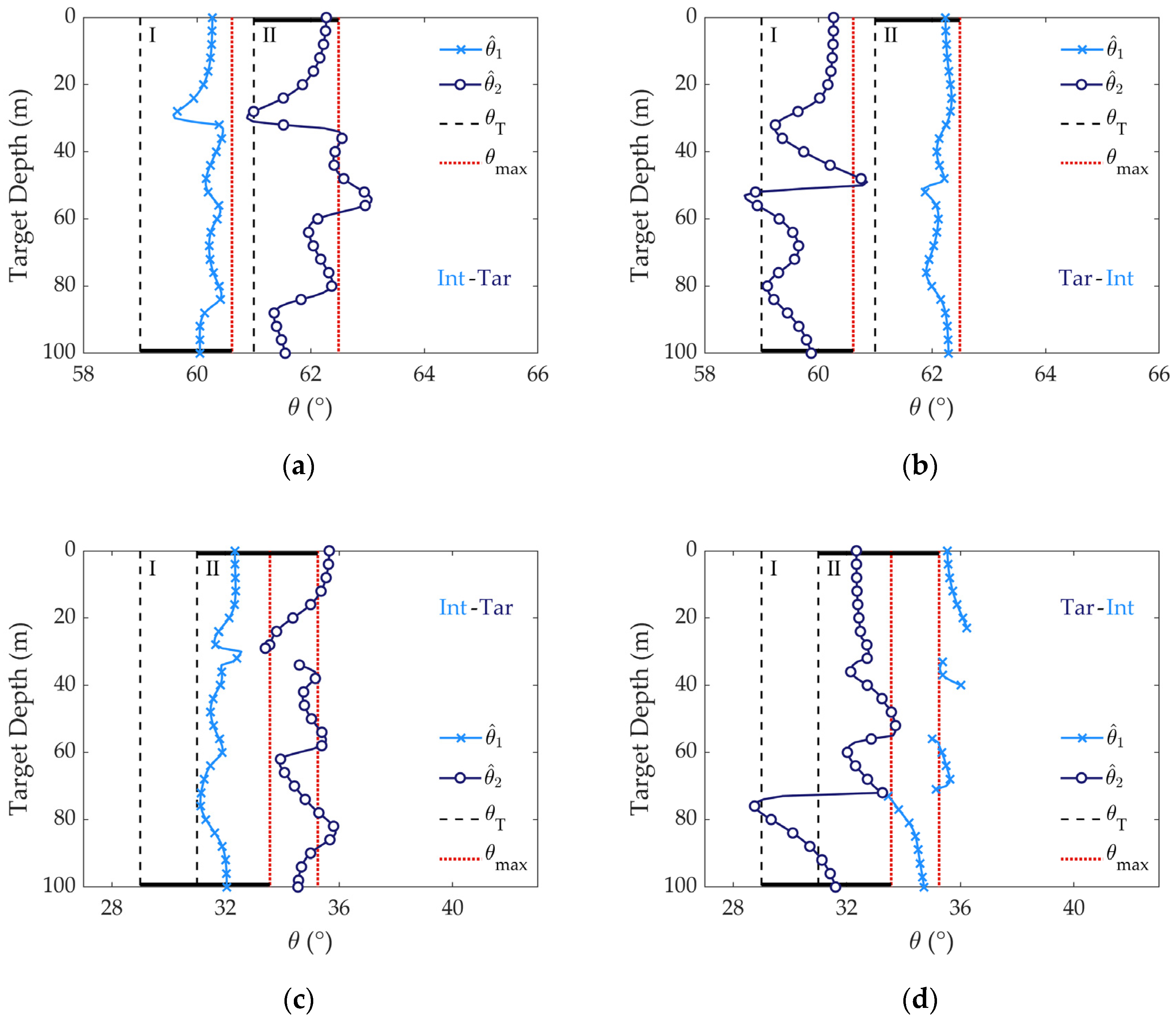
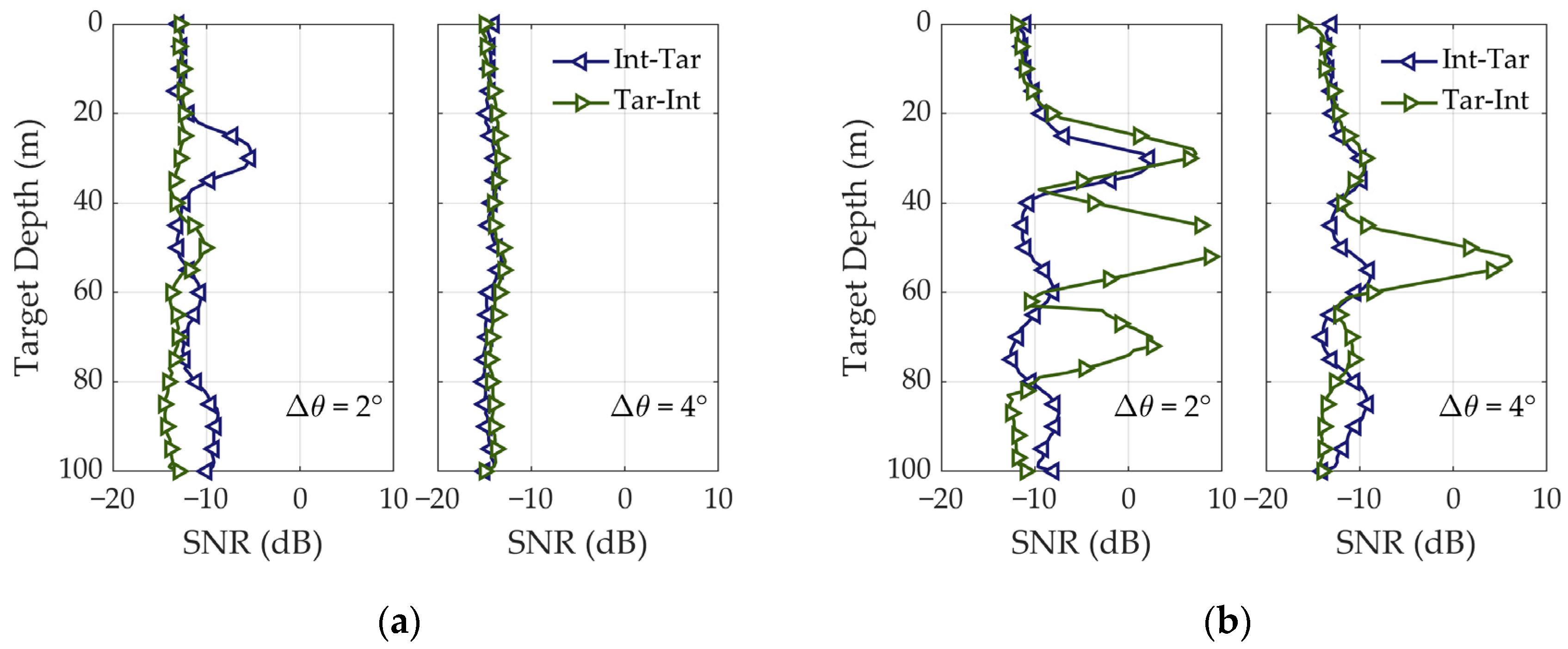
• In the presence of a near-surface interferer, the bearing estimation performance is significantly influenced by the target position. Primarily, it could be attributed to the multimode mechanism and shows distinct dependence on the target–interferer angular arrangement;
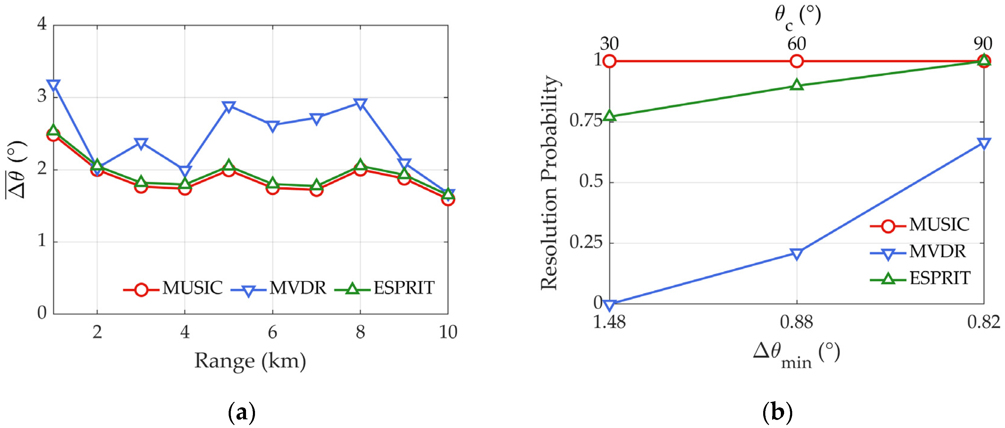
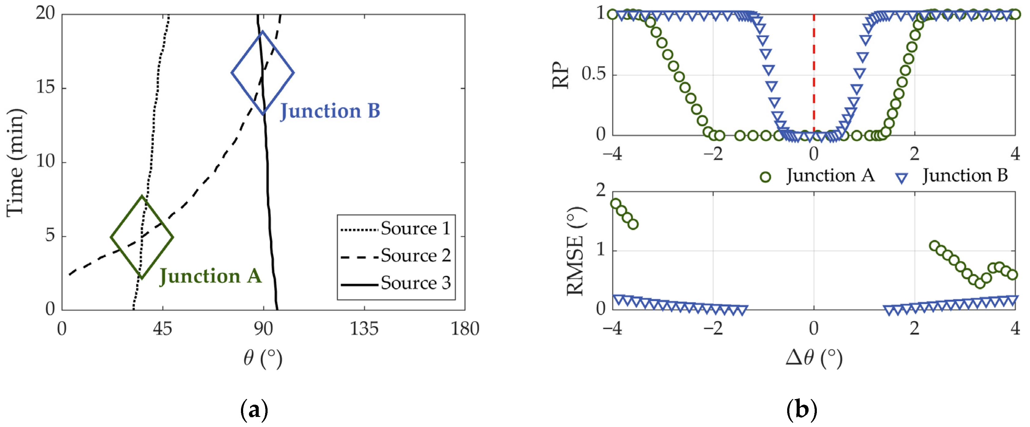
• Since junction B is near the broadside direction, the minimum angular separation for complete resolution gets smaller. By designating $\Delta \theta$ = 0° as the central axis, symmetrical characteristics can be detected, which indicates that bearing deviation barely occurs. Before and after the track crossing, the minimum angular separation is 1.43° and 1.49°, respectively;
• However, in terms of junction A, the deviating bearing estimation results in asymmetric characteristics. And in order to completely resolve the sources, the required minimum angular separations before and after their track crossing are 3.59° and 2.39°, respectively;
• From the aspect of bearing estimation accuracy of the target, the bearing deviation also governs. It is notable that more significant variation can be observed for bearing estimates around junction A. Before the track crossing, the averaged RMSE is about 1.72°, while it is reduced to about 0.71° after the crossing. In addition, compared with the estimates obtained by the use of measured sound speed, RMSE is decreased by 79% and 62%, respectively. For junction B, the RMSE is no more than 0.2° in the considered interval of $\Delta \theta \in$[–4, 4]°, and the decrease achieved by reference sound speed substitution is around 54%.

For detection and identification of underwater sources by the coarray-based MUSIC algorithm, the bearing estimation performance was acquired through experimental data. Particularly, on account of underwater source bearing estimation by horizontal arrays, one of the most difficult conditions involves the interesting weak signal being masked by interferers, especially when their angular separation gets smaller. By inducing the resolution performance under different target–interferer positions, the application guidance of ECSA is concluded.

5. Summary and Discussion

In order to solve the problem of target identification in the angular domain, methods such as the MUSIC algorithm can be used for the presence of a target among the noise and interference background, especially when the target signal and interference source are at adjacent bearings. Generally, the ECSA is capable of providing a helpful sparse configuration for applications of DOA estimation with the use of substantially fewer sensors. Nevertheless, limitation occurs for the underwater bottom-mounted ECSA, which is attributed to the multimode mechanism. In this paper, the conducted ECSA spanned an aperture of 393.75 m. Then, the SS technique was carried out, which made it possible to perform the MUSIC method in the difference-coarray domain efficiently. On that basis, the performance of underwater bearing estimation was numerically analyzed. It was thus shown that the resolution performance is greatly influenced by angular separation between the sources. Additionally, it is also related to true bearing and relative position of the sources, especially their angular arrangement. On one hand, for target movements near the sea surface, the feature of bearing estimation barely fluctuates with the target depth, and near-broadside targets could induce fewer losses of performance. On the other hand, when the target depth is different from that of the interferer, especially lower than the upper boundary of the thermocline, the corresponding bearing deviation is less pronounced than that of the near-surface interferer. As a result, resolution performance differs remarkably as their angular arrangement exchanges. Moreover, on the occasion that the MUSIC algorithm is capable of distinguishing the target from interferers, the bearing estimation could be refined by substituting the reference sound speed based on target position.

With regard to sources in the angular domain, the characteristics of resolution performance and estimation accuracy have been verified by experimental data. Typically, for a non-broadside junction formed by the track crossing of sources, the resolution probability curve is asymmetrical along the central axis, which reveals the influence of bearing deviation. In addition, by designating the reference sound speed in consideration of the multimode mechanism, more accurate target bearing estimation can be derived.

For the purpose of extensively applying ECSA in the underwater environment, bearing estimation methods with improved performance should be developed in the future, aiming to precisely identify targets in variable and complicated conditions.

References

1. Vaidyanathan, P.P.; Pal, P. Sparse sensing with co-prime samplers and arrays. IEEE Trans. Signal Process. 2010, 59, 573–586. [Google Scholar] [CrossRef]
2. Pal, P.; Vaidyanathan, P.P. Coprime sampling and the MUSIC algorithm. In Proceedings of the IEEE DSP/SPE Workshop, Sedona, AZ, USA, 4–7 January 2011; pp. 289–294. [Google Scholar]
3. Pal, P.; Vaidyanathan, P.P. Gridless methods for underdetermined source estimation. In Proceedings of the IEEE 48th Asilomar Conference on Signals, Systems and Computers, Pacific Grove, CA, USA, 2–5 November 2014; pp. 111–115. [Google Scholar]
4. Zheng, W.; Zhang, X.; Gong, P.; Zhai, H. DOA estimation for coprime linear arrays: An ambiguity-free method involving full DOFs. IEEE Commun. Lett. 2017, 22, 562–565. [Google Scholar] [CrossRef]
5. Yang, T.C.; Ye, Z. Array gain of coprime arrays. J. Acoust. Soc. Am. 2019, 146, EL306–EL309. [Google Scholar] [CrossRef] [PubMed]
6. Qin, S.; Zhang, Y.D.; Amin, M.G. Generalized coprime array configurations for direction-of-arrival estimation. IEEE Trans. Signal Process. 2015, 63, 1377–1390. [Google Scholar] [CrossRef]
7. Adhikari, K.; Buck, J.R.; Wage, K.E. Beamforming with extended co-prime sensor arrays. In Proceedings of the IEEE ICASSP, Vancouver, BC, Canada, 26–31 May 2013; pp. 4183–4186. [Google Scholar]
8. Adhikari, K.; Buck, J.R.; Wage, K.E. Extending coprime sensor arrays to achieve the peak side lobe height of a full uniform linear array. EURASIP J. Adv. Signal Process. 2014, 2014, 148. [Google Scholar] [CrossRef]
9. Moghadam, G.S.; Shirazi, A.B. Direction of arrival (DOA) estimation with extended optimum co-prime sensor array (EOCSA). Multidimens. Syst. Signal Process. 2022, 33, 17–37. [Google Scholar] [CrossRef]
10. Chen, X.; Zhang, H.; Gao, Y.; Wang, Z. DOA estimation of underwater acoustic co-frequency sources for the coprime vector sensor array. Front. Mar. Sci. 2023, 10, 1211234. [Google Scholar] [CrossRef]
11. Chen, X.; Zhang, H.; Lv, Y. Improving the beamforming performance of a vector sensor line array with a coprime array configuration. Appl. Acoust. 2023, 207, 109329. [Google Scholar] [CrossRef]
12. Wang, L.; Zhao, H.; Wang, Q. Underwater sparse acoustic sensor array design under spacing constraints based on a global enhancement whale optimization algorithm. Appl. Sci. 2022, 12, 11825. [Google Scholar] [CrossRef]
13. Dong, F.; Xu, L.; Li, X.; Wang, S.; Xie, X. Particle filter algorithm for underwater acoustic source DOA tracking with co-prime array. In Proceedings of the 2019 IEEE International Conference on Mechatronics and Automation (ICMA), Tianjin, China, 4–7 August 2019; pp. 2445–2450. [Google Scholar]
14. Pan, J.; Sun, M.; Dong, X.; Wang, Y.; Wang, Y.; Zhang, X. Enhanced DOA estimation with co-prime array in the scenario of impulsive noise: A pseudo snapshot augmentation perspective. IEEE Trans. Veh. Technol. 2023, 72, 11603–11616. [Google Scholar] [CrossRef]
15. Pan, H.; Pan, J.; Zhang, X.; Wang, Y. Time-delay estimation of ground penetrating radar using co-prime sampling strategy via atomic norm minimization. IEEE Trans. Instrum. Meas. 2024, 73, 8502812. [Google Scholar] [CrossRef]
16. Su, Y.; Wang, X.; Lan, X. Co-prime array interpolation for DOA estimation using deep matrix iterative network. IEEE Trans. Instrum. Meas. 2024, 73, 2533912. [Google Scholar] [CrossRef]
17. Liu, C.L.; Vaidyanathan, P.P. Remarks on the spatial smoothing step in coarray MUSIC. IEEE Signal Process. Lett. 2015, 22, 1438–1442. [Google Scholar]
18. Chen, T.; Guo, M.; Guo, L. A direct coarray interpolation approach for direction finding. Sensors 2017, 17, 2149. [Google Scholar] [CrossRef]
19. Zheng, Z.; Huang, Y.; Wang, W.Q.; So, H.C. Spatial smoothing PAST algorithm for DOA tracking using difference coarray. IEEE Signal Process. Lett. 2019, 26, 1623–1627. [Google Scholar]
20. Wang, M.; Nehorai, A. Coarrays, MUSIC, and the Cramér-Rao bound. IEEE Trans. Signal Process. 2016, 65, 933–946. [Google Scholar]
21. Wang, M.; Zhang, Z.; Nehorai, A. Performance analysis of coarray-based MUSIC and the Cramér-Rao bound. In Proceedings of the IEEE ICASSP, New Orleans, LA, USA, 5–9 March 2017; pp. 3061–3065. [Google Scholar]
22. Chen, C.; Yang, K.; Duan, R.; Ma, Y. Acoustic propagation analysis with a sound speed feature model in the front area of Kuroshio Extension. Appl. Ocean Res. 2017, 68, 1–10. [Google Scholar] [CrossRef]
23. Liu, J.; Piao, S.; Zhang, M.; Zhang, S.; Guo, J.; Gong, L. Characteristics of three-dimensional sound propagation in Western North Pacific fronts. J. Mar. Sci. Eng. 2021, 9, 1035. [Google Scholar] [CrossRef]
24. Liu, Y.; Chen, Y.; Meng, Z.; Chen, W. Performance of single empirical orthogonal function regression method in global sound speed profile inversion and sound field prediction. Appl. Ocean Res. 2023, 136, 103598. [Google Scholar]
25. Yang, T.C. Beam intensity striations and applications. J. Acoust. Soc. Am. 2003, 113, 1342–1352. [Google Scholar] [CrossRef]
26. Lakshmipathi, S.; Anand, G.V. Subspace intersection method of high-resolution bearing estimation in shallow ocean. Signal Process. 2004, 84, 1367–1384. [Google Scholar]
27. Yang, K.; Li, H.; He, C.; Duan, R. Error analysis on bearing estimation of a towed array to a far-field source in deep water. Acoust. Aust. 2016, 44, 429–437. [Google Scholar]
28. Lu, Y.; Yang, K.; Liu, H.; Huang, C. Effect of emergence angle on acoustic transmission in a shallow sea. Arch. Acoust. 2020, 45, 3–9. [Google Scholar]
29. Wu, Y.; Zhang, W.; Hu, Z.; Zhang, W.; Zhang, B.; Wang, J.; Guo, W.; Xu, G.; Zhu, M. Directional response of a horizontal linear array to an acoustic source at close range in deep water. Acoust. Aust. 2022, 50, 91–103. [Google Scholar]
30. Jensen, F.B.; Kuperman, W.A.; Porter, M.B.; Schmidt, H. Computational Ocean Acoustics, 2nd ed.; Springer: New York, NY, USA, 2011; pp. 338–341. [Google Scholar]
31. Gong, Z.; Lin, J.; Guo, L. The effect of acoustic waves’ phase speed on preciseness of DOA estimation in shallow water. Acta Acust. 2002, 27, 492–496. [Google Scholar]
32. Premus, V.E.; Helfrick, M.N. Use of mode subspace projections for depth discrimination with a horizontal line array: Theory and experimental results. J. Acoust. Soc. Am. 2013, 133, 4019–4031. [Google Scholar]
33. Porter, M.B. The KRAKEN Normal Mode Program; Naval Research Lab.: Washington, DC, USA, 1992. [Google Scholar]
34. Conan, E.; Bonnel, J.; Nicolas, B.; Chonavel, T. Using the trapped energy ratio for source depth discrimination with a horizontal line array: Theory and experimental results. J. Acoust. Soc. Am. 2017, 142, 2776–2786. [Google Scholar]
35. Zhang, W.; Wu, Y.; Shi, J.; Leng, H.; Zhao, Y.; Guo, J. Surface and underwater acoustic source discrimination based on machine learning using a single hydrophone. J. Mar. Sci. Eng. 2022, 10, 321. [Google Scholar] [CrossRef]
36. Zhai, D.; Zhang, B.; Li, F.; Zhang, Y.; Yang, X. Passive source depth estimation in shallow water using two horizontally separated hydrophones. Appl. Acoust. 2022, 192, 108723. [Google Scholar]
37. Jensen, J.K.; Hjelmervik, K.T.; Østenstad, P. Finding acoustically stable areas through Empirical Orthogonal Function (EOF) classification. IEEE J. Ocean. Eng. 2012, 37, 103–111. [Google Scholar]
38. Chen, C.; Lei, B.; Ma, Y.L.; Duan, R. Investigating sound speed profile assimilation: An experiment in the Philippine Sea. Ocean Eng. 2016, 124, 135–140. [Google Scholar]
Figure 1. Schematic of a typical ECSA structure: (1) an ECSA consisting of two subarrays with (A, B) = (2, 3); (2) difference coarray; (3) central ULA part of the difference coarray.
Jmse 13 00633 g001
Figure 2. Schematic diagram of the HLA (the ECSA samples are based on the uniform HLA) and source configuration in the experimental scene, with measured sedimental coefficients noted.
Jmse 13 00633 g002
Figure 3. Illustration of mode trapping phenomenon: (a) measured SSP from September 2020 and corresponding depth-dependent normal mode functions, with refracting and reflecting separately marked separately; (b) modal transmission loss with respect to propagation range.
Jmse 13 00633 g003
Figure 4. Simulation results of DOA estimation by using the ECSA (coprime pair of arrays, A = 5, B = 7): (a) comparison of normalized spatial spectrum (true source bearings are [20, 30, 40, 42, 50, 60, 70, 80]°); (b) resolution probability for different source angular separations (central angles are representatively selected as 30°, 60°, and 90°).
Jmse 13 00633 g004
Figure 5. DOA estimation by the use of ECSA: (a) feature of bearing deviation (bearing estimates are denoted by colorful marks, and interval θ T , θ max is highlighted by black bar on the θ axis); (b) bearing estimation accuracy with respect to source depth and propagation range (estimation error Δ θ is averaged over the five bearing angles).
Jmse 13 00633 g005
Figure 6. Performance comparison of relevant DOA algorithms by the use of ECSA: (a) mean bearing estimation error with respect to propagation range; (b) resolution probability for different source angular separations and central angles.
Jmse 13 00633 g006
Figure 7. Analytical simulation of impact of SSP characteristics: (a) schematic curves of the four typical SSPs; (b) mean bearing estimation error difference between the two source groups with respect to propagation range.
Jmse 13 00633 g007
Figure 8. Analytical simulation of sound speed fluctuations on the basis of EOF reconstruction: (a) accessed Argo profiles near the experimental area; (b) cumulative contribution rate (R) of the first six EOFs and depth-dependent curves of the first four EOFs; (c) twenty reconstructed SSPs by the use of random EOF coefficients; (d) mean bearing estimation error difference between the two typical source groups with respect to propagation range.
Jmse 13 00633 g008
Figure 9. With respect to the source angular separation Δ θ , the resolution performance of the MUSIC estimator (results of co-planar far-field narrow-band sources are denoted by dashed and dotted lines, while contrastive results in the underwater waveguide are denoted by solid lines with specific markers): (a) SD = 7 m, 7 m; (b) SD = 35 m, 35 m; (c) SD = 35 m, 7 m; (d) SD = 7 m, 35 m.
Jmse 13 00633 g009
Figure 10. In the condition of Δ θ = 2° and ID = 7 m, bearing estimates with respect to the target depth (interval θ T , θ max is highlighted by black bar on the θ axis): (a) θ c = 60°, Int-Tar; (b) θ c = 60°, Tar-Int; (c) θ c = 30°, Int-Tar; (d) θ c = 30°, Tar-Int.
Jmse 13 00633 g010
Figure 11. Under different Δ θ and source arrangement, the minimum tolerable SNR for complete resolution, with target distance randomly selected in [2, 20] km (averaged over 1000 trials): (a) θ c = 60°; (b) θ c = 30°.
Jmse 13 00633 g011
Figure 12. For 1000 trials, the source resolution ratio in conditions of different angular separations within 2°, ID = 7 m, and SNR = 10 dB, while TD is randomly selected inside the water column and target distance randomly selected in [2, 20] km, SNR = 0 dB: (a) θ c = 60°; (b) θ c = 30°.
Jmse 13 00633 g012
Figure 13. On the premise of correct resolution for target with arbitrary depth and distance and target bearing estimation error with respect to the angular separation: (a) taking no account of the target position; (b) reference sound speed decided depending on the target position.
Jmse 13 00633 g013
Figure 14. Schematic diagram of the experimental scene. Together with the SSP in the water column, the sound speed, density, and attenuation of the sediment are also denoted, namely c s = 1596 m/s, ρ s = 1.64 g/cm3, and α s = 0.46 dB/λ.
Jmse 13 00633 g014
Figure 15. Experimental presentation (central frequency f 0 = 120 Hz, bandwidth W = 10 Hz): (a) 20-min source tracks during the experiment (target: sources 1 and 3; interferer: source 2); (b) bearing estimation result, which is focused on the aspect of resolution performance and target bearing estimation accuracy (before track crossing: Δ θ < 0 ; after track crossing: Δ θ > 0 ).
Jmse 13 00633 g015