Experimental Investigation into the Effects of Deep-Sea Environment on Thermophysical Properties of Hydraulic System Working Fluids

Abstract

The thermophysical properties of working fluids serve as a fundamental basis for the design and analysis of subsea hydraulic systems. Precise characterization of hydraulic oil properties—including bulk modulus, thermal conductivity, and viscosity—is critical for optimizing system efficiency and energy conservation in deep-sea applications. However, no existing model accurately describes the variation patterns of these parameters across full-ocean-depth pressure ranges (0.1–110 MPa) and wide temperature intervals (2–70 °C). In this study, No. 10 aviation hydraulic oil was selected as the test medium. An experimental apparatus was developed to measure its properties, with subsequent data analysis revealing distinct temperature- and pressure-dependent trends. Empirical equations for bulk modulus, thermal conductivity, and viscosity–temperature–pressure relationships were derived, achieving coefficients of determination (R²) of 97.96%, 98.27%, and 94.608%, respectively.

1. Introduction

The deep sea harbors abundant marine mineral and biological resources, representing a valuable asset for human sustainable development. The exploitation of these marine resources necessitates reliable equipment and technology for support [1,2]. Benefiting from its small size, lightweight design, and stepless speed regulation, the deep-sea hydraulic power source is widely utilized in propulsion systems for subsea equipment [3,4,5,6,7]. Its transmission system demonstrates characteristics such as high structural stiffness, compact design, strong load-bearing capacity, superior power-to-weight ratio, and rapid response, making it a crucial power source for deep-sea applications including scientific sampling [8,9,10], mineral resource exploitation [11,12,13], and underwater robotics [14,15,16].

The bulk modulus of hydraulic oil, a crucial parameter influencing the natural frequency, stiffness, as well as static and dynamic characteristics and control accuracy of hydraulic systems is significantly affected by deep-sea conditions [17,18,19,20,21,22]. Moreover, the bulk modulus of liquids exhibits notable temperature dependence [23,24] and pressure dependence [25,26]. The gas content has a substantial impact on the bulk modulus of oil at low pressures [27,28,29]. In deep-sea operating environments, changes in temperature and pressure alter the bulk modulus of oil, subsequently influencing the dynamic response of hydraulic systems [30,31].

The bulk modulus of liquids is primarily classified into isothermal and isentropic types [32,33]. During stable operation and descent from sea level to operating depth, the underwater hydraulic system maintains thermal equilibrium with the ambient environment [34,35,36], equivalent to isothermal compression [37,38]. During operation, particularly in plunger pumps, hydraulic oil compression occurs over extremely short durations, rendering its working process akin to isentropic compression [39]. However, experimentally simulating an adiabatic and isentropic environment where compression is instantaneously completed is challenging; thus, isothermal compression is often used as a substitute, with negligible errors for engineering applications. Various methods exist to measure bulk modulus variations with temperature and pressure, including the compression method [40,41,42,43], sonic velocity method [21,44,45,46], mass variation method [47,48], and ultrasonic grating method [49,50,51,52,53]. Currently, however, no device employing these methods measures the bulk modulus under full-ocean-depth and wide-temperature-range conditions, nor is there a theoretical model accurately describing oil bulk modulus variations [47].

In marine environments, the thermal conductivity of hydraulic oil is influenced by the coupled effects of temperature and pressure. Current measurement techniques for liquid thermal conductivity are primarily categorized into steady-state and transient methods. Steady-state methods include guarded hot plate, heat flux sensors, and hot box techniques, whereas transient methods encompass hot-wire, probe, hot disk, transient plane source, and laser flash approaches [54,55]. Researchers have employed various techniques, such as spectral analysis by Hendrix et al. for transparent liquids [56], point heating by Watanabe et al. for molten salts [57], and consistency comparisons among hot-wire transient, photon spectroscopy, and laser flash methods by Kwon et al. [58]. Kobatake, H. et al. quantified the thermal conductivity of molten silicon via non-contact modulated laser calorimetry [59]. The 3-Omega method has proven effective for measuring cryogenic liquid thermal conductivity [60,61]. Chen et al. developed an improved thermal pulse technique suitable for microscale liquid characterization, particularly nanofluids, albeit limited by dielectric film thermal conductivity and thickness [62]. Mendiola-Curto et al. employed thermoelectric module impedance spectroscopy for liquid thermal conductivity evaluation [63]. Bioucas investigated the temperature-dependent thermal conductivity of glycerol at 0.1 MPa [64]. The transient hot-wire method has been extensively validated for both gaseous and liquid media [65,66]. Kutcherov observed a pressure-dependent linear relationship in crude oil thermal conductivity at 1 GPa, monotonically increasing with pressure [67]. Alharbi et al. demonstrated a positive correlation between thermal conductivity and temperature for water at atmospheric pressure (0.1 MPa) within the range of 0–32 °C [68]. However, systematic studies on the pressure and temperature dependence of hydraulic oil thermal conductivity under deep-sea conditions are scarce. Systematic characterization of these dependencies is crucial for optimizing the design of future deep-sea hydraulic systems.

The functionality of the hydraulic system, encompassing energy and heat transfer, as well as mechanical component lubrication, is reliant on the working fluid. An appropriate viscosity of this fluid minimizes internal leakage within the system [69]. Currently, hydraulic oil and water-based liquids are the primary working fluids utilized in hydraulic systems [70,71,72,73]. Notably, the viscosity of these fluids exhibits a substantial dependence on both pressure and temperature [74,75,76,77]. Underwater hydraulic equipment operates across a broad spectrum of temperatures and pressures. Variations in operating depth and temperature alter the viscosity of the oil, influencing the output power, efficiency, and overall performance of the equipment [78,79,80]. Excessively low viscosity can augment leakage, while excessively high viscosity may elevate friction losses and heat dissipation [81]. In deep-sea environments, friction power losses stemming from viscous fluids significantly contribute to the decrement in system efficiency [82]. Disregarding fluid viscosity variations can lead to an underestimation of the heat exchanger length by approximately 20% during the design phase [83]. Lower viscosity results in decreased pressure peaks within the oil film of a plunger pump’s plunger pair [84]. When the operating depth reaches 11 km, the viscosity of aviation hydraulic oil No. 10 is approximately 15–20 times that under normal temperature and pressure conditions. The maximum motion delay of deep-sea valve-controlled hydraulic cylinders (VCHCS) can reach up to 52.5% [85,86].

As a transmission medium, low viscosity is essential, whereas as a lubricating medium, high viscosity is preferred. Thus, a balance between these two requirements is crucial [87]. Currently, various methods exist for predicting liquid viscosity characteristics. These include estimation through empirical formulas [88]; presumptive determination based on molecular structure [89,90]; modeling based on material properties and molecular dynamics (MD) [91]; viscosity measurements using viscometers and rheometers [92,93]; and employing optical methods to measure the viscosity of working fluids [94].

This study first presents the design and analysis of a test apparatus for measuring the bulk modulus and thermal conductivity of hydraulic oil under full-ocean-depth conditions. Subsequently, the bulk modulus, thermal conductivity, and viscosity of No. 10 aviation hydraulic oil are experimentally characterized over a temperature range of 2 °C to 70 °C and a pressure range of 0.1 MPa to 110 MPa. Finally, theoretical analyses are conducted to elucidate the variation trends of these parameters under deep-sea conditions based on the experimental results. The measured data and analytical conclusions provide critical insights and theoretical support for the high-precision design, optimization, and precise control of marine hydraulic systems in future applications.

2. Measurement Principles and Apparatus

2.1. Measurement Principles and Device Design for Bulk Modulus of Elasticity and Thermal Conductivity

This study employs a compression method to measure the bulk modulus of No. 10 aviation hydraulic oil. To ensure compact dimensions and structural integrity of the measurement apparatus, the cylindrical vessel was fabricated from 17–4PH precipitation-hardened stainless steel. This material selection enables a thin-walled design that facilitates thermal equilibrium between the internal and external environments while maintaining minimal mass. During initial hydraulic oil filling, entrapped gases were evacuated from the test chamber through a dedicated vent port to eliminate non-condensable gas interference. A manually operated high-pressure pump pressurized the system, driving piston displacement to compress the oil within the test cavity. Upon reaching the target pressure, the shut-off valve was closed, and the system stabilized. Piston displacement was then quantified via a linear variable differential transformer (LVDT), enabling calculation of the compressed liquid volume. The bulk modulus of the hydraulic oil under specified pressure–temperature conditions was subsequently derived using the constitutive equation:

$$\beta =-V{\left({\displaystyle \frac{\partial P}{\partial V}}\right)}_T$$

(1)

where β denotes the bulk modulus, V the initial volume, and əP/əV the pressure–volume gradient at a constant temperature T. The testing system is illustrated in Figure 1.

Since materials undergo deformation in response to changes in pressure and temperature, a deformation analysis of the test chamber under various pressure and temperature conditions was conducted using ANSYS Workbench 2020 R2. The fundamental material parameters are presented in

Table 1. Pressure chamber parameters.

Name	Parameter
Yield strength	930 MPa
Tensile strength	725 MPa
Outside diameter	100 mm
Thickness of sensor cabin wall	20 mm
Piston diameter	40 mm
Cabin height	500 mm

.

The structure of the test object influences the accuracy of static analysis to a certain extent. Therefore, in this simulation analysis, different meshes were employed to conduct a mesh independence analysis, aiming to calculate the impact of various mesh scales on the accuracy of static analysis under the same operating condition, thereby selecting the most suitable mesh scale. The dependence of the deformation of the barrel on different mesh scales was investigated under the conditions of a temperature of 2 °C and a pressure of 110 MPa. The mesh sizes and quantities are presented in the

Table 2. Mesh size and number.

Type	A	B	C	D
Mesh size	1	5	10	15
Mesh number	1,388,629	52,444	12,042	9773
Volume change	3.703494445	3.72950696	5.530856984	6.762874003

.

With the reduction in mesh size and the increase in mesh number, the maximum difference between the simulation results of type B mesh and type A mesh was below 1%. The results indicate that, in this scenario, all meshes can be used at an acceptable level. Ultimately, to balance numerical accuracy and computational resources, this study selects the type B mesh with a mesh size of 5 mm.

Based on simulation analysis data, it was observed that the volume expansion of the test chamber exhibited a linear increase with rising temperature under fixed pressure. The trend of its variation is shown in Figure 2. Similarly, at a constant temperature, the volume expansion also increased linearly with the augmentation of internal pressure. Under normal atmospheric pressure of 0.1 MPa and an ambient temperature of 2 °C, the volumetric contraction of the test chamber was relatively minor. As the internal pressure within the chamber increased, the internal volume expanded, at which point pressure became the dominant factor influencing the volumetric changes of the test chamber. The maximum volume change occurred at an internal pressure of 110 MPa and a temperature of 70 °C, where the test chamber’s volume increased by approximately 4.32 mm³. The internal volume of the test chamber was 376,991.1184 mm³. The impact of volumetric changes in the test chamber due to environmental variations on the overall volume was minimal, accounting for only 0.0011%. Therefore, the error caused by this device in subsequent measurements of the bulk modulus of oil is negligible.

The CLMZ4 type wire-drawing displacement sensor employed in this experiment utilizes resistance values to represent the displacement of the piston, featuring a theoretically infinite resolution and a temperature drift coefficient of ±0.0025%/K. The water bath temperature control precision of the measurement setup is ±0.1 °C. The elastic deformation of the sealing ring under maximum pressure is approximately 10%. Considering the combined maximum volume change and various primary errors, the maximum error in the measurement of the bulk modulus of elasticity is approximately 0.9%. The modulus of elasticity can be neglected.

The thermal conductivity of hydraulic oil under varying operational conditions was measured using a DRE-III multifunctional rapid thermal conductivity analyzer. The probe was encapsulated within a custom-built high-pressure chamber and connected to the testing instrument via a watertight electrical connector. The opposing end of the chamber was interfaced with a pressure intensifier pump through high-pressure hydraulic tubing to generate the required test pressures. Key instrumentation parameters are detailed in

Table 3. Basic parameters of DRE-III thermal conductivity tester.

Name	Parameter
Measurement range of thermal conductivity	0.001–500 W/(m·K)
Resolution	0.0001 W/(m·K)
Measurement error	≤3%
Test duration	5–300 s
Temperature range for sample testing	−40–130 °C

.

The probe was fabricated from nickel wire, whose bulk modulus of 180 GPa rendered the mechanical deformation induced by the maximum deep-sea pressure (110 MPa) negligible, as this pressure constituted merely 0.061% of the material’s bulk modulus. Consequently, pressure-induced measurement errors could be systematically disregarded. The sensing element demonstrated sufficient metrological precision to satisfy the measurement requirements for the target specimens under investigation. The measurement system in the laboratory is shown in Figure 3.

2.2. Viscosity Measurement Principles and Devices

The laboratory testing instrument employed was the Viscolab-PVT system, which is capable of precisely characterizing the viscosity of working fluids under diverse operational conditions and varying working depths in subsea hydraulic systems. The experimental instrument is shown in Figure 4, and

Table 4. Technical parameters of the test apparatus.

Name	Parameter
Model	Viscolab pvt
Range	0.02–10,000 cP
Precision	±1% (full scale)
Repeatability	Count ± 0.8%
Maximum pressure	20,000 psi
Pressure fluctuation	≤0.1 MPa
Temperature range	0–190 °C
Temperature fluctuation	≤±0.5 °C

lists the key parameters.

2.3. Selection of Oil Samples and Measurement Points for Testing

The test liquids included No. 10 aviation hydraulic oil and deionized water. Temperature control was achieved using a circulating water bath. The pressure testing range covered static pressures from sea level to a depth of 11,000 m in the abyss, with test pressure points at 0.1 MPa, 21 MPa, 35 MPa, 55 MPa, 75 MPa, 90 MPa, and 110 MPa. Deep-sea temperatures lie between 2 °C and 4 °C [95], while the optimal operating temperature for hydraulic systems generally ranges from 30 °C to 60 °C, not exceeding 80 °C as the maximum [96,97]. The selected test temperature points were 2 °C, 30 °C, 50 °C, and 70 °C.

3. Results and Discussion

3.1. Measurement and Analysis of Bulk Elastic Modulus

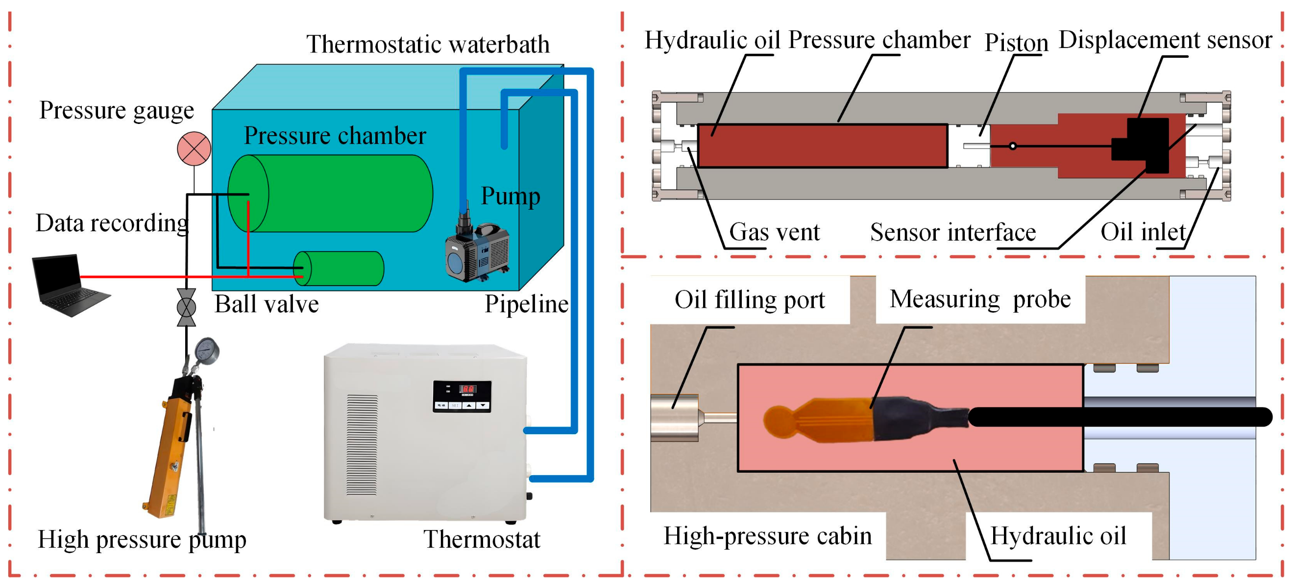
The experimental setup designed in this paper maintains a constant temperature using a thermostatic water bath and measures the bulk modulus of elasticity by varying the pressure at a fixed temperature. Therefore, the isothermal secant bulk modulus of elasticity was selected to calculate the bulk modulus values of the working fluid under different operating conditions. The test fluid was No. 10 aviation hydraulic oil. In practical engineering applications, most of the hydraulic oil under natural conditions contains dissolved gases, with only a small number of insoluble bubbles. Furthermore, in deep-sea applications, as pressure increases, gases gradually dissolve into the oil, a phenomenon which does not significantly affect the overall bulk modulus of elasticity of the hydraulic oil. Therefore, this paper measures the bulk modulus of elasticity of hydraulic oil under normal operating conditions.

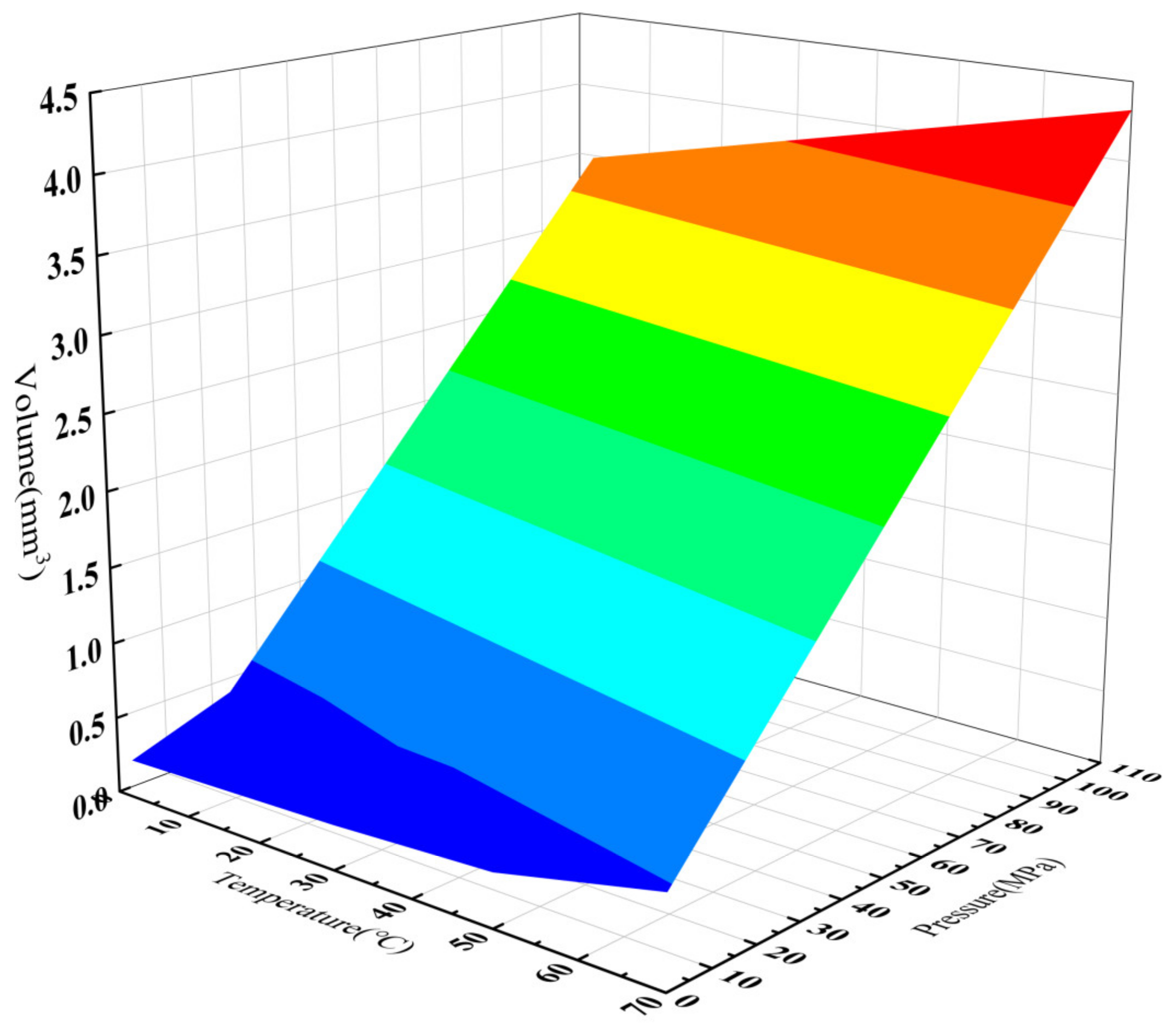
The actual measured density of No. 10 aviation hydraulic oil at 20 °C in daily use environments is 830.4 kg/m³, and the density at 2 °C is 850 kg/m³. Using the density at 2 °C as the baseline, the laboratory measured changes in the density of the hydraulic oil based on variations in volume at different temperatures and pressures. The initial length inside the test chamber was 268 mm, and, given the internal diameter of 40 mm, the initial volume was 338,343.9518 mm³. The initial mass was 0.287592359 kg. The volume changes and densities of No. 10 aviation hydraulic oil measured in the laboratory are shown in

Table 5. Average volume change of hydraulic oil.

Volume Change of Hydraulic Oil (mm3)
	2 °C	30 °C	50 °C	70 °C
0.1 MPa	0	−3233.073951	−14,769.26964	−17,634.94882
21 MPa	4555.695112	4261.779299	3967.863485	3306.552904
35 MPa	8376.60069	7862.248016	7421.374296	6392.668948
55 MPa	11,830.1115	10,801.40615	10,360.53243	9552.263945
75 MPa	15,504.05917	14,769.26964	14,401.87487	13,667.08534
90 MPa	19,413.13949	18,663.65417	18,443.21731	17,781.90673
110 MPa	22,631.51765	21,676.29126	21,602.81231	21,161.93859

.

Since the initial volume and initial mass of the hydraulic oil under test were known, calculations could be performed using the relationship among density, volume, and mass. This experiment was conducted with an initial condition of 2 °C and 0.1 MPa. Under the condition of 0.1 MPa, as the temperature increased, the volume of the hydraulic oil expanded. In this paper, the expanded volume change was taken to be negative, and the compressed volume change was taken to be positive for calculations. The changes in density values are shown in

Table 6. Average density of hydraulic oil.

Hydraulic Oil Density (Kg/m3)
	2 °C	30 °C	50 °C	70 °C
0.1 MPa	850	841.954632	814.4480058	807.8915872
21 MPa	861.6011896	852.5922325	823.7038027	815.4661427
35 MPa	871.5782276	861.7909011	831.932721	822.665005
55 MPa	880.7968409	869.448478	839.0666748	830.168147
75 MPa	890.8203899	880.0046928	849.0780186	840.1473341
90 MPa	901.7390228	890.6176837	859.3311485	850.3693534
110 MPa	910.9313664	899.0049976	867.5213541	858.9539708

.

$${\displaystyle \frac{initial mass(\mathrm{m})}{original bulk(v)-volume change(\Delta v)}}=density(\rho )$$

(2)

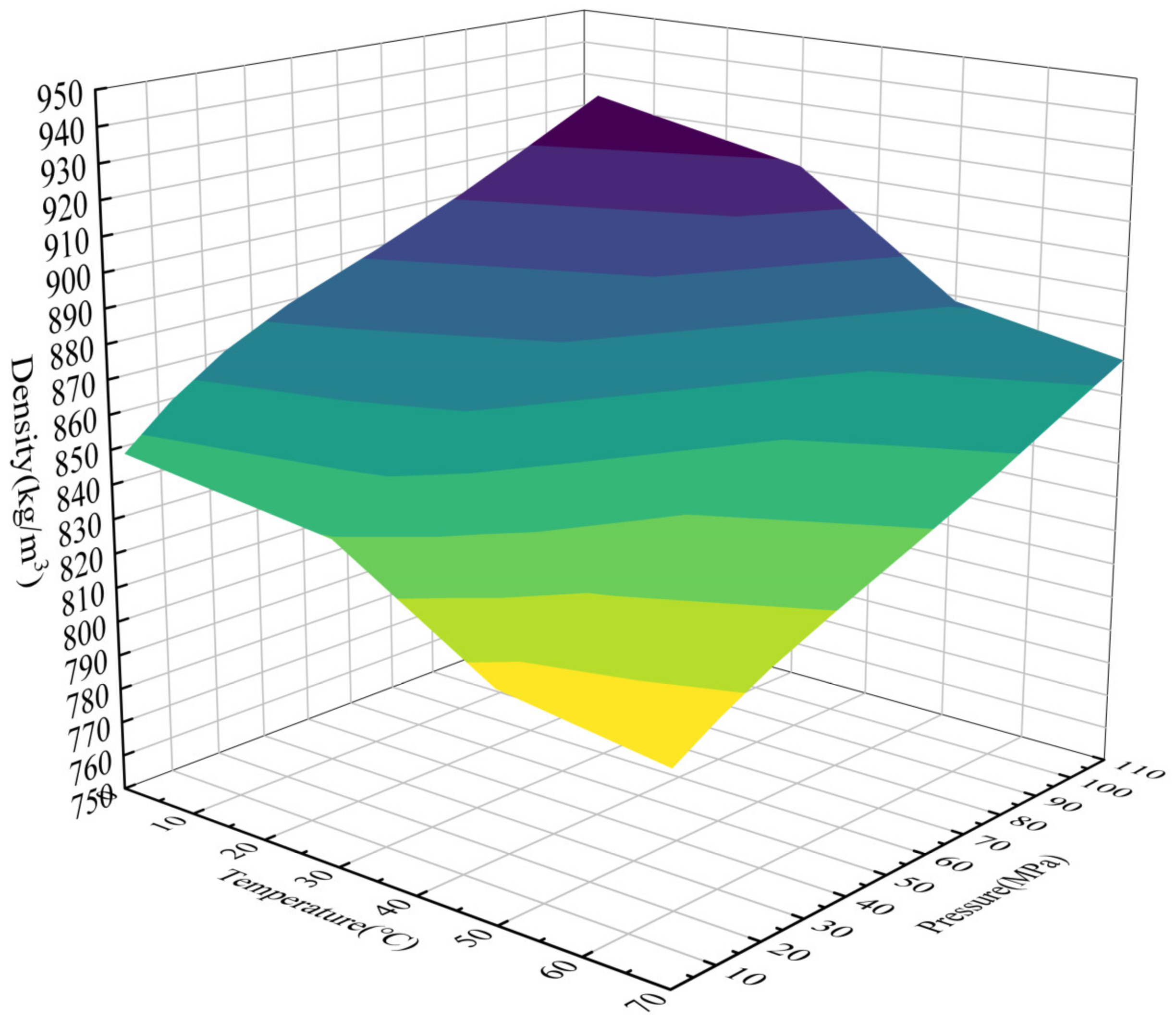
Based on the data in the table above, a graph depicting the variation in the density of No. 10 aviation hydraulic oil with temperature and pressure was plotted. This allowed for further analysis of the trend in density changes under different operating conditions in deep-sea environments and hydraulic systems. Its density variation with temperature and pressure is shown in Figure 5 and Figure 6, respectively.

The above analysis indicates that the density of hydraulic oil was minimal under high-temperature and low-pressure conditions and maximal under low-temperature and high-pressure conditions. At constant pressure, the liquid density decreased as the temperature increased. An increase in temperature augments the kinetic energy of liquid molecules, intensifying their irregular thermal motion, which, in turn, weakens the intermolecular interactions, increases the intermolecular distance, and reduces the number of molecules per unit volume, thereby lowering the liquid density. At constant temperature, the liquid density exhibited an approximately linear trend with changes in pressure. As pressure increased, the distance between liquid molecules decreased, enhancing intermolecular interactions; consequently, the liquid density increased with the increase in pressure.

The bulk modulus of elasticity of hydraulic oil under different operating conditions can be calculated based on the volume variation, initial volume, initial pressure, and pressure variation of the hydraulic oil being tested. The variations are shown in

Table 7. Average bulk modulus of hydraulic oil.

Bulk Modulus (MPa)
	2 °C	30 °C	50 °C	70 °C
21 MPa	742.683484	801.4892415	889.9328891	1076.586134
35 MPa	848.222716	912.3494357	999.1919764	1169.395283
55 MPa	1001.008174	1106.818476	1192.888766	1304.325508
75 MPa	1200.260986	1272.015264	1348.520755	1432.554129
90 MPa	1307.14542	1372.629213	1435.94749	1501.437273
110 MPa	1345.510987	1418.228421	1471.113551	1513.94925

.

We plotted a trend diagram of the variation in the bulk modulus of elasticity of aviation hydraulic oil No. 10, as it changed under different conditions based on the data.

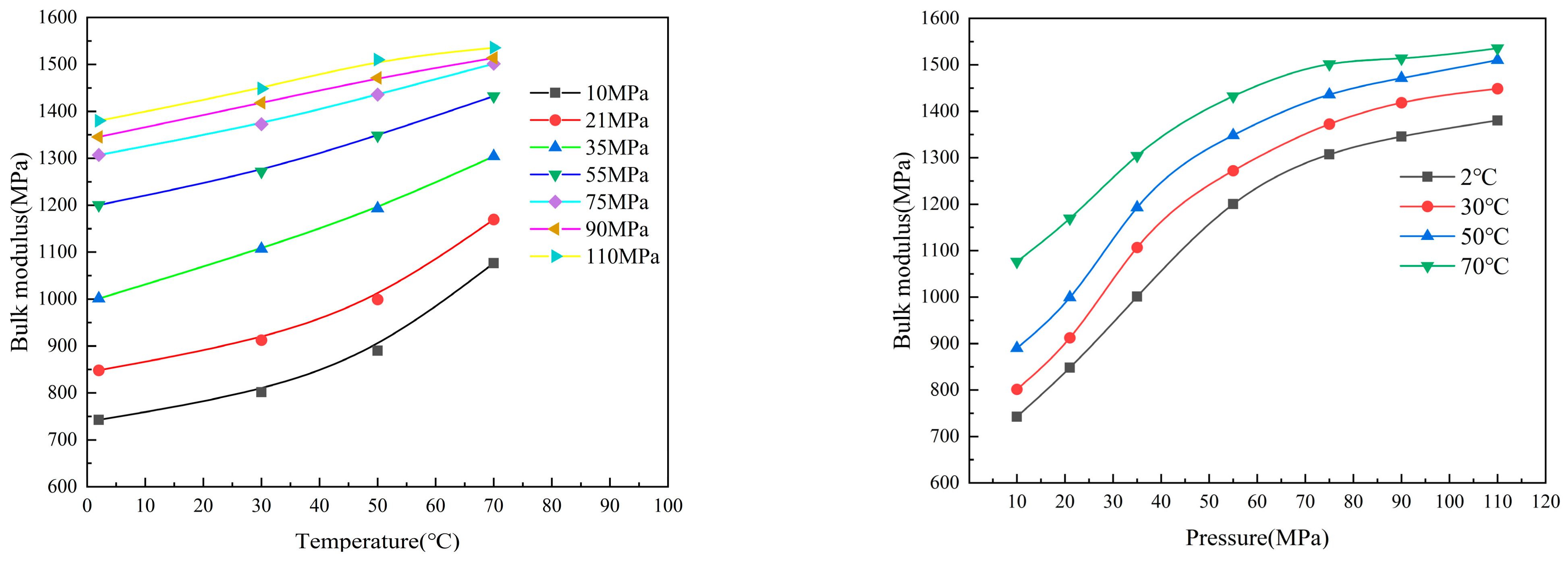
As shown in Figure 7 and Figure 8, the bulk modulus of elasticity of aviation hydraulic oil No. 10 reached its maximum under high-temperature and high-pressure conditions and its minimum under low-temperature and low-pressure conditions. Under constant pressure conditions, the higher the pressure, the greater the bulk modulus of elasticity. When the pressure was less than 35 MPa, the increase in the bulk modulus of elasticity between 2 °C and 30 °C was approximately linear and relatively slow. When the temperature exceeded 30 °C, the rate of increase in the bulk modulus of elasticity accelerated with increasing temperature. When the pressure was higher than 35 MPa, the bulk modulus of elasticity increased linearly with increasing temperature, and the higher the pressure, the slower the rate of increase in the bulk modulus of elasticity with temperature. Under constant temperature conditions, the higher the temperature, the greater the bulk modulus of elasticity. When the pressure was less than 55 MPa, the bulk modulus of elasticity increased rapidly with increasing pressure, with an increase rate approximately three times higher than that under high pressure. When the pressure exceeded 55 MPa, the rate of increase in the bulk modulus of elasticity slowed down with further increases in pressure. The trend in the bulk modulus of elasticity of the oil indicates that, as the submergence depth of an underwater hydraulic system increases, the system stiffness increases rapidly down to a certain depth, beyond which the rate of increase in system stiffness slows down, and the deeper the depth, the smaller the change in system stiffness.

Currently, the commonly used models for the bulk modulus of elasticity of oil include the Wylie model [98], the Nykanen model [99], the Ruan model [100], and the AMESim model [101], among others.

(a)

Wylie Model

$$E={\displaystyle \frac{E_0}{1+\alpha {\left(\frac{p_0}{p}\right)}^{1/\lambda }\left(\frac{E_0}{\lambda p}-1\right)}}$$

(3)

In the equation, E₀ represents the bulk modulus of pure hydraulic oil under atmospheric pressure; α denotes the air content in the oil; P₀ is one standard atmosphere; and λ represents the specific heat ratio of air.

(b)

Nykanen Model

$$E={\displaystyle \frac{\alpha {\left(\frac{p_0}{p}\right)}^{1/\lambda }+\frac{1-\alpha }{1+\frac{p-p_0}{E_0}}}{\frac{\alpha {\left(\frac{p_0}{p}\right)}^{1/\lambda }}{\lambda p}+\frac{1-\alpha }{{\left(1+\frac{p-p_0}{E_0}\right)}^2{E}_0}}}$$

(4)

(c)

Ruan Model

$$E=\left\{\begin{array}{l}{\displaystyle \frac{E_0}{\alpha p_0{E}_0\left(\frac{1}{p^2}-\frac{1}{p_{\mathrm{c}}^2}\right)+1}},p_0<p<p_{\mathrm{c}}\\ E_0,p⩾p_{\mathrm{c}}\end{array}\right.$$

(5)

In the equation, p_c represents the critical pressure.

(d)

AMESim Model

$$E={\displaystyle \frac{\frac{C_1(1-\phi )}{{\rho }_{\mathrm{L}}}+\frac{C_2\theta +C_3\phi }{p^{1/\lambda }}}{\frac{C_1}{{\rho }_{\mathrm{L}}}\left(\frac{1-\phi }{E_0}+\frac{\mathrm{d}\phi }{\mathrm{d}p}\right)+\frac{C_2}{p^{1/\lambda }}\left(\frac{\theta }{\lambda p}-\frac{\mathrm{d}\theta }{\mathrm{d}p}\right)+\frac{C_3}{p^{1/\lambda }}\left(\frac{\phi }{\lambda p}-\frac{\mathrm{d}\phi }{\mathrm{d}p}\right)}}$$

(6)

In the equation, θ represents the proportion of air released within the hydraulic oil; φ denotes the proportion of vapor released within the hydraulic oil; and ${\rho }_L$ stands for the density of pure oil.

The existing models exhibited an inadequate performance in characterizing the bulk modulus of the tested hydraulic oil. Consequently, a second-order polynomial (Poly2D) model was implemented in the Origin 2021 software to derive an empirical equation correlating the bulk modulus with temperature and pressure, based on experimental data and graphical analysis. The fitted equation achieved a coefficient of determination (R²) of 97.96% against measured values, demonstrating its capability to accurately describe the coupled temperature–pressure dependence of the bulk modulus within the validated operational range of 0.1–110 MPa and 2–70 °C.

$$E=569.63+2.82\times T+14.94\times P+0.037\times T^2-0.066\times P^2-0.03\times T\times P$$

(7)

In the equation, E (MPa) represents the bulk modulus of elasticity of the oil; T (°C) denotes the temperature of the oil; and P (MPa) indicates the pressure applied to the oil.

3.2. Measurement and Analysis of Thermal Conductivity

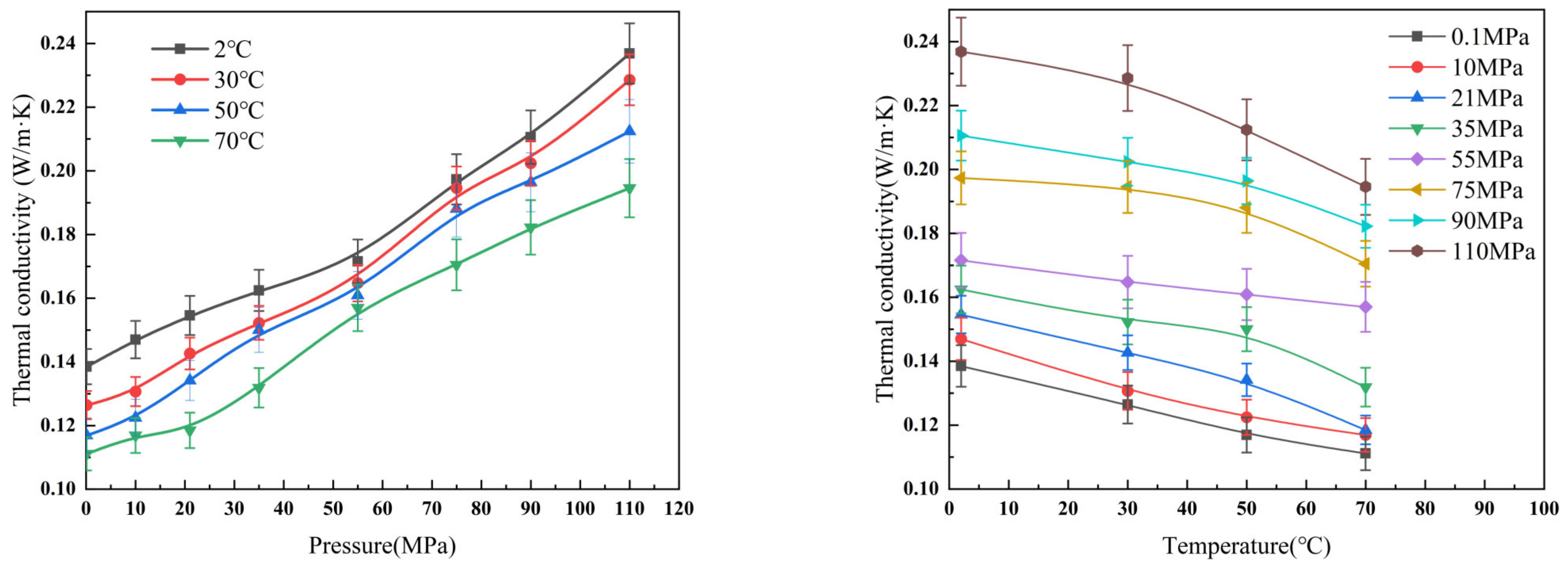
A graph was plotted depicting the variations in the thermal conductivity of aviation hydraulic oil No. 10 as measured in the laboratory under different operating conditions, as shown in Figure 9 and Figure 10.

As evidenced by the graphical analysis, the thermal conductivity of hydraulic oil attained its minimum value under high-temperature, low-pressure conditions and its maximum under low-temperature, high-pressure regimes. Prior studies have established that thermal conductivity is inversely proportional to the square root of the liquid molecular mass. Elevated temperatures induce thermal expansion, thereby increasing intermolecular distances and weakening molecular interactions, in turn reducing thermal transport efficiency. Conversely, pressure elevation compresses intermolecular spacing, enhancing heat transfer efficacy. Under isothermal conditions, thermal conductivity exhibited an approximately linear increase with pressure across all tested temperature ranges, with similar pressure-dependent growth rates observed at different temperatures. Conversely, under isobaric conditions, thermal conductivity decreased with rising temperature, albeit at a diminishing rate that approximated a linear behavior. Comparative analysis revealed that thermal conductivity at 110 MPa was approximately double the value measured at atmospheric pressure (0.1 MPa), while a temperature increase from 2 °C to 70 °C resulted in a reduction of approximately 20%. These findings indicate that temperature dominates thermal conductivity variations under ambient pressure, whereas pressure becomes the primary influencing factor under high-pressure conditions.

Based on the measured data and plotted results, a second-order polynomial (Poly2D) model was employed in the Origin software to derive an empirical equation correlating thermal conductivity with temperature and pressure. The fitted equation demonstrated excellent agreement with the experimental data, achieving a coefficient of determination (R²) of 98.27%. This model accurately characterized the coupled temperature–pressure dependence of thermal conductivity across the validated operational envelope of 0.1–110 MPa and 2–70 °C.

$$\lambda =0.1349-2.934\times {10}^{-4}\times T+4.3869\times {10}^{-4}\times P-1.3387\times {10}^{-6}\times T^2+4.29\times {10}^{-6}\times P^2-6.27\times {10}^{-7}\times T\times P$$

(8)

where λ represents the thermal conductivity, T denotes the temperature, and P stands for pressure.

3.3. Measurement and Analysis of Viscosity

The viscosity of Kunlun No. 10 aviation hydraulic oil was measured under various temperatures and pressure points in a deep-sea environment, using the oil as a sample. The measurement results are shown in

Table 8. The viscosity value of Kunlun No. 10 aviation hydraulic oil (cP).

	Viscosity (cP)
	2 °C	30 °C	50 °C	70 °C
0.1 MPa	41.94	28.71	21.14	16.36
21 MPa	52.71	34.23	24.29	17.87
35 MPa	63.97	39.58	26.82	19.22
55 MPa	85.97	46.37	30.01	20.86
75 MPa	116.33	55.42	33.66	22.55
90 MPa	144.32	63.25	36.43	24.03
110 MPa	185.99	75.82	40.67	26.34

.

Based on the data in Table 8, viscosity–temperature, viscosity–pressure, and viscosity–temperature–pressure graphs for the hydraulic oil were plotted, as shown in Figure 11 and Figure 12. These graphs provide further analysis of the viscosity trends in the hydraulic oil under different working conditions in deep-sea environments with varying temperatures and pressures, as well as on mobile exploration platforms.

Based on the viscosity–temperature correlation, it is evident that, under constant pressure conditions, the viscosity of the hydraulic oil diminishes as the temperature increases. Conversely, at a fixed temperature, an increase in pressure leads to an increase in the hydraulic oil’s viscosity. Moreover, with the intensification of pressure, the viscosity’s variation with temperature at constant pressure exhibits progressively more nonlinear characteristics. Specifically, under constant pressure scenarios, the rate of viscosity change with temperature is minimal at atmospheric pressure, amounting to 0.376 cP/°C, whereas it peaks at 2.347 cP/°C under 110 MPa. This signifies that elevated pressure amplifies the rate of viscosity alteration. Notably, the rate of change at high pressures is 6.24 times that observed at low pressures. As temperature increases across various pressure levels, the viscosity tends to decrease, and the ultimate viscosity values converge. This convergence suggests that pressure exerts a more pronounced influence on viscosity at lower temperatures, whereas at higher temperatures, its impact on viscosity diminishes in significance, with temperature emerging as the primary determinant of viscosity values.

Based on the viscosity–pressure behavior of hydraulic oil, it is discernible that, at a fixed temperature, an elevation in pressure results in an increase in the oil’s viscosity. As the temperature escalates, the impact of pressure on viscosity diminishes, causing the viscosity values to converge. At a constant temperature, the maximum rate of change in viscosity with respect to pressure is observed at lower temperatures, amounting to 1.309 cP/MPa, whereas the minimum rate occurs at higher temperatures, reaching 0.09 cP/MPa. This signifies that the rate of viscosity alteration at low temperatures is approximately 14.5 times that observed at high temperatures. Under low-pressure conditions, the variation in viscosity across varying temperatures is relatively insignificant. However, as pressure increases, the divergence in viscosity values across different temperatures becomes increasingly evident. Notably, at low temperatures, the viscosity undergoes substantial shifts, and its relationship with pressure is nonlinear. This underscores the primary role of pressure in determining viscosity at low temperatures, whereas at high temperatures, viscosity is predominantly governed by temperature, resulting in a stronger tendency for viscosity values to converge at identical temperatures across different pressures. At low temperatures, the disparity in viscosity values across different pressures intensifies.

In examining the viscosity–temperature–pressure relationship of No. 10 hydraulic oil, as illustrated in Figure 12, a notable trend emerges: the viscosity reaches its maximum under conditions of low temperature and high pressure, while it diminishes to its minimum at high temperatures and low pressures. The difference in viscosity between these conditions is substantial, with a maximum spread of 169.63 cP. Conversely, under conditions of either low temperature and low pressure or high pressure and high temperature, the viscosity values are comparatively low and exhibit minimal discrepancy. This observation highlights the intricate interplay between temperature and pressure in influencing the viscosity of the hydraulic oil. Furthermore, it is noteworthy that, depending on specific operational conditions or scenarios depicted in Figure 3, the viscosity of the hydraulic fluid may be predominantly governed by a single factor, either temperature or pressure.

The Reynolds equation, Slotte equation, Walther equation, Vogel equation, and Barus equation are widely used to describe the physical properties of hydraulic oil. The Reynolds equation is accurate within a limited temperature range, but its parameters are difficult to determine [102]; the Slotte equation is used for numerical calculations [103]; the Walther equation forms the basis of the ASTM viscosity–temperature. However, the equation mainly focuses on the viscosity–temperature relationship without fully considering the influence of pressure [104]; the Vogel equation is relatively accurate under high pressures and is widely used in engineering applications [105]; the Barus equation is most commonly used to describe the viscosity–pressure characteristics of fluids, indicating that viscosity increases exponentially with pressure, and it represents the change in dynamic viscosity of hydraulic oil with pressure [106]. P.W. Gold et al. studied the viscosity–temperature-pressure behavior of mineral oils and integrated the Vogel equation into the viscosity–pressure equation based on the Barus equation, but the equation has seven unknown parameters to be determined, making it not universally applicable for describing the viscosity–temperature–pressure behavior of mineral oils [107]. The Cheng and Sternlicht equation contains many unknown parameters and is currently used less frequently [108]. These relationship equations are listed in

Table 9. Common hydraulic oil viscosity temperature pressure relationship equations.

Name	Equation
Roelands	${\displaystyle \frac{\ln \mu +1.2}{\ln {\mu }_0+1.2}}={\left({\displaystyle \frac{t_0+135}{t+135}}\right)}^s{\left(1+{\displaystyle \frac{p}{2000}}\right)}^x$
Slotte	${\mu }_0={\displaystyle \frac{a}{{\left(b+T_A\right)}^c}}$
Walther	$\lg \left[\lg \left(v+0.8\right)\right]=a+b\lg T$
Vogel	${\mu }_0=K\exp \left({\displaystyle \frac{B}{t+C}}\right)$
Barus	$\mu ={\mu }_0{\mathrm{e}}^{\alpha p}$
P.W. Gold	$\eta =K\exp \left[{\displaystyle \frac{B}{v+C}}\right]\exp \left[{\displaystyle \frac{p}{a_1+a_{2}v+\left(b_1+b_{2}v\right)p}}\right]$
Cheng and Sternlicht	$\mu ={\mu }_0\exp \left(ap+{\displaystyle \frac{\beta }{t}}-{\displaystyle \frac{\beta }{t_0}}+{\displaystyle \frac{\gamma p}{t}}\right)$

.

In Table 9, the viscosity–temperature index of Roelands is relatively difficult to determine, while other expressions have more coefficients to be determined, leading to more complex calculations. Furthermore, their current application range is narrower compared to Barus’ formula. Therefore, this paper selects the viscosity values calculated using Barus’ formula for comparative analysis with the experimentally measured viscosity values. A comparative analysis was conducted using the fitted values and measured values at various pressures at 30 °C.

As it can be seen in

Table 10. Error analysis of fitted parameter values versus measured values.

Pressure	Barus	Measurement	Error
0.1 Mpa	16.72 (cP)	28.71 (cP)	42%
21 Mpa	43.57 (cP)	34.23 (cP)	−27%
35 Mpa	36.405 (cP)	39.58 (cP)	8%
55 Mpa	55.415 (cP)	46.37 (cP)	−20%
75 Mpa	93.6 (cP)	55.42 (cP)	−69%
90 Mpa	125.455 (cP)	63.25 (cP)	−98%
110 Mpa	153.285 (cP)	75.82 (cP)	−102%

, the maximum deviation between the fitted data and the measured values reached 102%, with the minimum error being 8%. The empirical formula exhibits poor fitting performance for the viscosity values of the hydraulic oil used in this paper, making it unsuitable for practical engineering applications. Therefore, this paper performs formula fitting based on the measured values within the experimental conditions.

A second-order polynomial (Poly2D) model was employed in the Origin software to develop a viscosity–temperature–pressure (VTP) empirical equation for No. 10 aviation hydraulic oil, based on the acquired experimental data and corresponding graphical representations. The fitted equation achieved a coefficient of determination (R²) of 94.608% against measured values, demonstrating its capability to accurately characterize the coupled temperature–pressure dependence of viscosity across the validated operational envelope of 0.1–110 MPa and 2–70 °C.

$$\begin{array}{l}{\mu }_{oil}=46.12-1.57T+0.8P+0.019T^2+0.0028p^2-0.017TP\\ 0 °\mathrm{C}\le T\le 70 °\mathrm{C};0.1MP\mathrm{a}\le P\le 110MP\mathrm{a}\end{array}$$

(9)

where $\mu$ (cP) represents the viscosity of the working fluid and $T$ (°C) represents the ambient temperature.

4. Conclusions

This study presents an experimental setup designed to measure the bulk modulus of elasticity and thermal conductivity of oil under ultra-high pressure (up to 110 MPa) and within a wide temperature range (2 °C to 70 °C). Systematic measurements were conducted on Kunlun No. 10 aviation hydraulic oil to investigate the trends in its bulk modulus of elasticity, thermal conductivity, and viscosity across pressure ranges from 0.1 MPa to 110 MPa and temperatures from 2 °C to 70 °C. Furthermore, a comprehensive analysis was performed to explore how these parameters vary with temperature and pressure.

Based on experimental data, a viscosity–temperature–pressure model for hydraulic oil was established, with temperature and pressure as independent variables, revealing the influence of environmental parameters on the physical properties of the working fluid. Notably, the values in each equation are solely functions of pressure and temperature, without any irrelevant variables, thus simplifying the calculation process compared to other existing models. The correlation coefficients (R²) between the fitted results and actual measured values for the bulk modulus of elasticity, thermal conductivity, and viscosity are 97.96%, 98.27%, and 94.608%, respectively, meeting the precision requirements for engineering design applications. The findings of this study provide valuable theoretical and data support for the design, optimization, and practical engineering applications of future underwater hydraulic equipment. They also serve as a reference for future research on mathematical models of various physical parameters of different working fluids in underwater hydraulic systems.

References

1. Kalyan, B.; Pallayil, V.; Vishnu, H. Underwater Exploration and Mapping. In Proceedings of the 2022 IEEE/OES Autonomous Underwater Vehicles Sym posium (AUV), Singapore, 19–21 September 2022; pp. 1–7. [Google Scholar]
2. Mirza, J.; Atieh, A.; Kanwal, B.; Ghafoor, S.; Almogren, A.; Kanwal, F.; Aziz, I. Relay aided UWOC-SMF-FSO based hybrid link for underwater wireless optical sensor network. Opt. Fiber Technol. 2025, 89, 104045. [Google Scholar]
3. Feng, Z.; Lam, J. Reduced-order dissipative filtering for discrete-time singular systems. In Proceedings of the 2013 IEEE International Symposium on Industrial Electronics, Taipei, Taiwan, 28–31 May 2013; pp. 1–6. [Google Scholar]
4. Jee, S.C.; Li, J.H.; Kim, J.T.; Lee, M.J.; Kang, H.J. Fault tolerant controller design of servo-valve controlled hydraulic propulsion systems. In Proceedings of the OCEANS 2015—Genova, Genova, Italy, 18–21 May 2015; pp. 1–5. [Google Scholar]
5. Wu, J.-B.; Li, L. Influence of ambient pressure on sealing performance of O-ring in deep-sea hydraulic system. Ocean Eng. 2022, 245, 110440. [Google Scholar]
6. Li, M.; Yu, C.; Zhang, X.; Liu, C.; Lian, L. Fuzzy adaptive trajectory tracking control of work-class ROVs considering thruster dynamics. Ocean Eng. 2023, 267, 113232. [Google Scholar]
7. Zhou, F.; Gu, L.; Luo, G.; Chen, J.; Zheng, M.; Shao, Z. Development of a hydraulic propulsion system controlled by proportional pressure valves for the 4500m work-class ROV. In Proceedings of the 2013 OCEANS—San Diego, San Diego, CA, USA, 23–27 September 2013; pp. 1–6. [Google Scholar]
8. Liu, Y.; Wu, D.; Li, D.; Deng, Y. Applications and Research Progress of Hydraulic Technology in Deep Sea. J. Mechan. Ical. Eng. 2018, 54, 14–23. [Google Scholar]
9. Wang, Y.; Guo, J.; Tan, X.; Chen, J.; Fang, Y.; Wang, W.; Ge, Y. Pore water pressure maintaining sampler for deployment on deep-sea ROV-Jellyfish. Deep. Sea Res. Part I Oceanogr. Res. Pap. 2024, 203, 104194. [Google Scholar]
10. Guo, J.; Wang, Y.; Wang, W.; Ren, X.; Zhou, P.; Fang, Y.; Deng, Y.; Chen, D.; Cao, J.; Zhang, C.; et al. Pressure-retaining sampler for sediment including overlying water based on heavy duty ROV-Jellyfish. Appl. Ocean Res. 2022, 128, 103354. [Google Scholar]
11. Kang, Y.; Liu, S. The Development History and Latest Progress of Deep-Sea Polymetallic Nodule Mining Technology. Minerals 2021, 11, 1132. [Google Scholar] [CrossRef]
12. Liu, B.; Wang, X.; Zhang, X.; Liu, J.; Liangwan, R.; Ma, Y. Research Status of Deep-Sea Polymetallic Nodule Collection Technol ogy. J. Mar. Sci. Eng. 2024, 12, 744. [Google Scholar]
13. Song, W.; Zhang, Y.; Zhu, X.; Zhao, G.; Xing, K. Design and Simulation of hydraulic system of the deep-sea miner. J. Phys. Conf. Ser. 2022, 2310, 12073. [Google Scholar]
14. Romano, C.; Gerard, D.; Edin, O.; Joseph, C.; Thomas, N.; Daniel, T. Inspection-Class Remotely Operated Vehicles—A Review. J. Mar. Sci. Eng. 2017, 5, 13. [Google Scholar] [CrossRef]
15. Chen, Y.; Zhang, Q.; Tian, Q.; Feng, X. Extended State Observer-Based Fuzzy Adaptive Backstepping Force Control of a Deep-Sea Hydraulic Manipulator with Long Transmission Pipelines. J. Mar. Sci. Eng. 2022, 10, 1467. [Google Scholar] [CrossRef]
16. Chen, G.; Yang, X.; Zhang, X.; Hu, H. Water hydraulic soft actuators for underwater autonomous robotic systems. Appl. Ocean Res. 2021, 109, 102551. [Google Scholar]
17. Wang, F.; Chen, Y. Design and experimental study of oil-based pressure-compensated underwater hydraulic system. Proc. Inst. Mech. Eng. Part I J. Syst. Control Eng. 2014, 228, 221–232. [Google Scholar]
18. Feng, H.; Du, Q.; Huang, Y.; Chi, Y. Modeling Study on Stiffness Characteristics of Hydraulic Cylinder under Multi-Factors. Stroj-Vestn.-J. Mech. Eng. 2017, 63, 447–456. [Google Scholar]
19. Gao, Y.; Shen, Y.; Xu, T.; Zhang, W.; Guvenc, L. Oscillatory Yaw Motion Control for Hydraulic Power Steering Articulated Vehicles Considering the Influence of Varying Bulk Modulus. IEEE Trans. Control Syst. Technol. 2019, 27, 1284–1292. [Google Scholar]
20. Chu, Z.; Chen, Y.; Zhu, D.; Zhang, M. Observer-based fault detection for magnetic coupling underwater thrusters with applications in jiaolong HOV. Ocean Eng. 2020, 210, 107570. [Google Scholar]
21. Geng, B.; Gu, L.; Liu, J. Novel Methods for Modeling and Online Measurement of Effective Bulk Modulus of Flowing Oil. IEEE Access 2020, 8, 20805–20817. [Google Scholar]
22. Wang, J.; Gong, G.; Yang, H. Control of bulk modulus of oil in hydraulic systems. In Proceedings of the 2008 IEEE/ASME International Conference on Advanced Intelligent Mechatronics, Xi’an, China, 2–5 July 2008; pp. 1390–1395. [Google Scholar]
23. Garai, J.; Laugier, A. The temperature dependence of the isothermal bulk modulus at 1bar pressure. J. Appl. Phys. 2007, 101, 023514. [Google Scholar] [CrossRef]
24. Yuan, X.; Wang, W.; Zhu, X.; Zhang, L. Theoretical Model of Dynamic Bulk Modulus for Aerated Hydraulic Fluid. Chin. J. Mech. Eng. Ji Xie Gong Cheng Xue Bao 2022, 35, 121. [Google Scholar]
25. Gholizadeh, H.; Bitner, D.; Burton, R.; Schoenau, G. Modeling and Experimental Validation of the Effective Bulk Modulus of a Mixture of Hydraulic Oil and Air. J. Dyn. Syst. Meas. Control 2014, 136, 051013. [Google Scholar]
26. Lunev, A.S.; Nikitin, A.; Kaizer, Y.F.; Lysyannikov, A.V.; Sokolov, D.A.; Obvintseva, V.Y. Comparative analysis of the dependence of the bulk elastic modulus of the liquid on pressure and gas factor. J. Phys. Conf. Ser. 2019, 1399, 055083. [Google Scholar] [CrossRef]
27. Sakama, S.; Tanaka, Y.; Goto, H. Mathematical model for bulk modulus of hydraulic oil containing air bubbles. Mech. Eng. J. 2015, 2, 15–00347. [Google Scholar] [CrossRef]
28. Yang, S.; Jiao, X.; Bao, Y.; Wang, W.; Ding, J. Fluid Air Content Affecting the Power Shift Performance of the Hydro-mechanical Variable Transmission. J. Mech. Eng. 2015, 51, 122–130. [Google Scholar] [CrossRef]
29. Yuan, X.; Zhu, X.; Wang, C.; Zhang, L. Research on Theoretical Model of Dynamic Bulk Modulus of Gas-Containing Hydraulic Oil. IEEE Access 2019, 7, 178413–178422. [Google Scholar] [CrossRef]
30. Kambic, M.; Kalb, R.; Tasner, T.; Lovrec, D. High Bulk Modulus of Ionic Liquid and Effects on Performance of Hydraulic System. Sci. World J. 2014, 2014, 504762. [Google Scholar] [CrossRef]
31. Ahart, M.; Hemley, R.J. Sound Velocity and Equation of State of Ballistic Gelatin by Brillouin Scattering. Materials 2023, 16, 1279. [Google Scholar] [CrossRef]
32. Chen, C. Design and Study of the Online Measuring Device for Hydraulic Oil Bulk Modulus. Master’s Thesis, Zhejiang University, Hangzhou, China, 2008. [Google Scholar]
33. Chen, S.Z. Study on Modeling and Simulation of Valve Controlled Cylinder Servo System for Hydraulic Bending Roll System. Master’s Thesis, Northeastern University, Shenyang, China, 2008. [Google Scholar]
34. Patil, V.C.; Acharya, P.; Ro, P.I. Experimental investigation of heat transfer in liquid piston compressor. Appl. Therm. Eng. 2019, 146, 169–179. [Google Scholar] [CrossRef]
35. Yan, G.; Jin, Z.; Yang, M.; Yao, B. The Thermal Balance Temperature Field of the Electro-Hydraulic Servo Pump Control System. Energies 2021, 14, 1364. [Google Scholar] [CrossRef]
36. Wang, Y.; Liang, C. Drilling Rig Hydraulic System Heat Balance Design. Meikuang Jixie (Coal Mine Mach.) 2014, 35, 44–46. [Google Scholar]
37. Park, J.-K.; Ro, P.I.; He, X.; Mazzoleni, A.P. Analysis, Fabrication, and Testing of a Liquid Piston Compressor Prototype for an Ocean Compressed Air Energy Storage (OCAES) System. Mar. Technol. Soc. J. 2014, 48, 86–97. [Google Scholar] [CrossRef]
38. Patil, V.C.; Acharya, P.; Ro, P.I. Experimental investigation of water spray injection in liquid piston for near-isothermal compression. Appl. Energy 2020, 259, 114182. [Google Scholar] [CrossRef]
39. Marshall, M.C.; Millot, M.; Fratanduono, D.E.; Sterbentz, D.M.; Myint, P.C.; Belof, J.L.; Kim, Y.J.; Coppari, F.; Ali, S.J.; Eggert, J.H.; et al. Metastability of Liquid Water Freezing into Ice VII under Dynamic Com pression. Phys. Rev. Lett 2021, 127, 135701. [Google Scholar] [CrossRef] [PubMed]
40. Hayward, A.T.J. Experimental Verification at High Pressure of the Relationship between Compression, Density and Sonic Velocity. Nature 1969, 221, 1047. [Google Scholar] [CrossRef]
41. Niezrecki, C.; Schueller, J.K.; Balasubramanian, K. Piezoelectric-based Fluid Bulk Modulus Sensor. J. Intell. Mater. Syst. Struct. 2004, 15, 893–899. [Google Scholar] [CrossRef]
42. Hruzík, L.; Burecek, A.; Vasina, M. Mathematical simulation and measurement of expansion of hydraulic hose with oil. Teh. Vjesn. 2017, 24, 1905–1914. [Google Scholar]
43. Bureček, A.; Hružík, L.; Vašina, M. Determination of Undissolved Air Content in Oil by Means of a Compression Method. Stroj-Vestn. J. Mech. Eng. 2015, 61, 477–485. [Google Scholar] [CrossRef]
44. Cho, B.H.; Lee, H.W.; Oh, J.S. Estimation technique of air content in automatic transmission fluid by measuring effective bulk modulus. Int. J. Auto Tech.-Kor. 2002, 3, 57–61. [Google Scholar]
45. Hetalo, A.M.; Rudenko, O.P.; Khorolskyi, O.V.; Samoilenko, S.O.; Bulavin, L.A. Temperature Dependence of the Bulk Elasticity Modulus of Aliphatic Alcohols and Their Fluorinated Analogs. Ukr. J. Phys. 2018, 63, 134. [Google Scholar] [CrossRef]
46. Voglhuber-Brunnmaier, T.; Niedermayer, A.O.; Jakoby, B. Localized sensing of bulk properties of oils. Mater. Today Proc. 2022, 62, 2648–2651. [Google Scholar] [CrossRef]
47. Kim, S.; Murrenhoff, H. Measurement of effective bulk modulus for hydraulic oil at low pressure. J. Fluids Eng. 2012, 134, 021201. [Google Scholar] [CrossRef]
48. Manring, N.D. The Effective Fluid Bulk-Modulus Within a Hydrostatic Transmission. J. Dyn. Syst. Meas. Control 1997, 119, 462–466. [Google Scholar]
49. Luna, D.A.; Real, M.A.; Durán, D.V. Undergraduate experiment to measure the speed of sound in liquid by diffraction of light. Am. J. Phys. 2002, 70, 874–875. [Google Scholar] [CrossRef]
50. Du, X. Laser-Ultrasonic Measurement of Single-Crystal Elastic Constants from Polycrystalline Samples by Measuring and Modeling Surface Acoustic Wave Velocities. Ph.D. Thesis, The Ohio State University, Columbus, OH, USA, 2018. [Google Scholar]
51. Li, C.; Hou, Z.-D.H.; Zhou, L.-X. Measuring the bulk elastic modulus of liquid by ultrasonic grating. Phys. Exp. 2018, 38, 56–59. [Google Scholar]
52. Mirza, J.; Kanwal, F.; Salaria, U.A.; Ghafoor, S.; Aziz, I.; Atieh, A.; Almogren, A.; Haq, A.U.; Kanwal, B. Underwater temperature and pressure monitoring for deep-sea SCUBA divers using optical techniques. Front. Phys. 2024, 12, 1417293. [Google Scholar] [CrossRef]
53. Lane, C.D.; Hathcock, D.J.; Leavitt, A.J.; Khan, F.A.; Hansen, J.E. Measurement of the Bulk Modulus of a Liquid Using a Pump?Probe Laser Technique. Chem. Educ. 2001, 6, 235–237. [Google Scholar] [CrossRef]
54. Xiang, Z. Research Status and Development Trend of Thermal Conductivity Measurement Methods. Appl. Phys. 2018, 8, 301–308. [Google Scholar]
55. Merritt, B.; Seneca, M.; Larson, S.; Davis, K.; Munro, T. Measurements of the thermal conductivity of reference liquids using a modified transient hot-wire needle probe. Int. J. Heat Mass Transf. 2022, 189, 122674. [Google Scholar] [CrossRef]
56. Hendrix, M.; Leipertz, A.; Simonsohn, G. Measurement of thermal-conductivity of transparent liquids by photon-correlation spectroscopy. Chem. Ing. Tech. 1984, 56, 334–335. [Google Scholar] [CrossRef]
57. Watanabe, A.; Susa, M.; Nagata, K. Thermal Conductivity Measurement on Liquid Using Spot Heating Method. J. Jpn. Inst. Met. Mater. 1994, 58, 982–983. [Google Scholar] [CrossRef]
58. Kwon, S.; Lee, J.; Kim, D.H. Reliability of thermal conductivity measurement of liquids by using transient hot-wire, photon-correlation spectroscopy and the laser flash method. J. Korean Phys. Soc. 2016, 68, 1145–1155. [Google Scholar] [CrossRef]
59. Kobatake, H.; Fukuyama, H.; Tsukada, T.; Awaji, S. Noncontact modulated laser calorimetry in a dc magnetic field for stable and supercooled liquid silicon. Meas. Sci. Technol. 2010, 21, 025901. [Google Scholar]
60. Hong, J.; Kim, D. Measuring the Thermal Conductivity of Flowing Liquid Samples Using the Three Omega Method. J. Heat Transf. 2012, 134, 094502. [Google Scholar]
61. Hamilton, B.; Brisson, J.G.; Iop, P.L. Modified 3ω conductivity technique for measurements of thermal conductivity in cryo-genic fluids. IOP Conf. Ser. Mater. Sci. Eng. 2024, 1301, 012164. [Google Scholar] [CrossRef]
62. Chen, S.; Zheng, F.; Li, J. Accurate measurement of thermal conductivity of micro-quantity liquids by dielectric transient current method. Appl. Therm. Eng. 2023, 230, 120830. [Google Scholar] [CrossRef]
63. Mendiola-Curto, V.; Beltrán-Pitarch, B.; García-Cañadas, J. Determination of thermal conductivity, thermal diffusivity, and spe cific heat of liquids using a thermoelectric module. Meas. Sci. Technol. 2024, 35, 045907. [Google Scholar]
64. Bioucas, F.E.B.; Koller, T.M.; Fröba, A.P. Thermal Conductivity of Glycerol at Atmospheric Pressure Between 268 K and 363 K by Using a Steady-State Parallel-Plate Instrument. Int. J. Thermophys. 2024, 45, 1–12. [Google Scholar]
65. Zhao, Z. Measuring and Modeling the Thermal Conductivity of High Temperature Liquids. Ph.D. Thesis, University of California San Diego, San Diego, CA, USA, 2021. [Google Scholar]
66. Salim, S.G.R. Thermal conductivity measurements using the transient hot-wire method: A review. Meas. Sci. Technol. 2022, 33, 125022. [Google Scholar]
67. Kutcherov, V.G. Thermal Conductivity of Oils at High Pressure. Chem. Technol. Fuels Oils 2023, 58, 973–976. [Google Scholar]
68. Alharbi, S.; Crepeau, J.; Rezaie, B.; Kumar, K. Temperature Dependence of Thermal Conductivity for Water Using the Transient Hot-Wire Method. J. Eng. Thermophys. 2022, 31, 78–97. [Google Scholar]
69. Tița, I.; Mardare, I.; Husaru, D.E. Theoretical aspects concerning working fluids in hydraulic systems. MATEC Web Conf. 2017, 112, 07014. [Google Scholar]
70. Nie, S.; Liu, X.; Ji, H.; Ma, Z.; Yin, F. Simulation and Experiment Study on Deformation Characteristics of the Water Hydraulic Flexible Actuator Used for the Underwater Gripper. IEEE Access 2020, 8, 191447–191459. [Google Scholar] [CrossRef]
71. Liu, Y.; Cheng, Q.; Wang, Z.; Pang, H.; Deng, Y.; Zhou, X.; Luo, X.; Cui, Y.; Wu, D. Seawater hydraulics: From the sea surface to depths of 11000 meters. Sci. China Technol. Sci. 2022, 65, 2178–2189. [Google Scholar] [CrossRef]
72. Radosavljevic, M.; Andelkovic, M.; Kocovic, P.; Petrovic, R.; Cvejic, S. An approach in reducing vibration in sea water hydraulic piston pumps for increased operational effectiveness and efficiency. Struct. Integr. Life 2022, 22, 275–279. [Google Scholar]
73. Chen, J.Y. Efficiency Analysis and Experimental Study on a Seawater Pump Used in VB System. Master’s Thesis, Huazhong University of Science and Technology, Wuhan, China, 2012. [Google Scholar]
74. An, H.; Sun, Y.; Zhu, W. Research on test method and correlation of low temperature performance of hydraulic oil. J. Phys. Conf. Ser. 2021, 1802, 022037. [Google Scholar] [CrossRef]
75. Wan, G.; Wu, Q.; Tang, M.; Lu, M.; Yang, K. Tribological Properties of Two Typical Materials of Hydraulic Motor’s Rotor at Different Ambient Temperatures. Appl. Sci. 2022, 12, 5582. [Google Scholar] [CrossRef]
76. Shen, M.; Zhang, F.; Liu, Y.; Zhou, X. Molecular dynamics study on the viscosity of hydraulic oil in the deep-sea environment. J. Mol. Liq. 2024, 411, 125716. [Google Scholar] [CrossRef]
77. Totten, G.E.; De Negri, V.J.; Negri, V.J.D. Handbook of Hydraulic Fluid Technology; Taylor & Francis Group: Baton Rouge, LA, USA, 2011. [Google Scholar]
78. Guo, M.; Liu, C.; Zhang, J.; Liu, S.; Yan, Q.; Khoo, B.C. Thermal effect on cavitation characteristics of a hydraulic torque converter. Numer. Heat Transf. Part A Appl. 2022, 82, 31–52. [Google Scholar] [CrossRef]
79. Niu, Y.; Gu, X.; Yue, X.; Zheng, Y.; He, P.; Chen, Q. Research on Thermodynamic Characteristics of Hydraulic Power Take-Off System in Wave Energy Converter. Energies 2022, 15, 1373. [Google Scholar] [CrossRef]
80. Ma, L.; Yan, H.; Ren, Y.; Li, L.; Cai, C. Numerical Investigation of Flow Force and Cavitation Phenomenon in the Pilot Stage of Electrical-Hydraulic Servo Valve under Temperature Shock. Machines 2022, 10, 423. [Google Scholar] [CrossRef]
81. Chen, Q.; Yu, H.; Yue, X.; Ye, Z.; Geng, D. Thermal-hydraulic modeling and simulation on wave energy power take-off system. Acta Energiae Solaris Sin. 2020, 41, 237–243. [Google Scholar]
82. Tian, Y.; Liu, S.; Long, J.; Chen, W.; Leng, J. Analysis and Experimental Research on Efficiency Characteristics of a Deep-Sea Hydraulic Power Source. J. Mar. Sci. Eng. 2022, 10, 1296. [Google Scholar] [CrossRef]
83. Kurmanova, D.; Jaichibekov, N.; Karpenko, A.; Volkov, K. Modelling and Simulation of Heat Exchanger with Strong Dependence of Oil Viscosity on Temperature. Fluids 2023, 8, 95. [Google Scholar] [CrossRef]
84. Patrosz, P. Influence of Properties of Hydraulic Fluid on Pressure Peaks in Axial Piston Pumps’ Chambers. Energies 2021, 14, 3764. [Google Scholar] [CrossRef]
85. Wu, J.-B.; Li, L.; Zou, X.-L.; Wang, P.-J.; Wei, W. Working Performance of the Deep-Sea Valve-Controlled Hydraulic Cylinder System under Pressure-Dependent Viscosity Change and Hydrodynamic Effects. J. Mar. Sci. Eng. 2022, 10, 362. [Google Scholar] [CrossRef]
86. Tian, Q.; Zhang, Q.; Chen, Y.; Huo, L.; Li, S.; Wang, C. Influence of Ambient Pressure on Performance of a Deep-sea Hydraulic Manipulator. In Proceedings of the OCEANS 2019—MARSEILLE, Marseille, France, 17–20 June 2019. [Google Scholar]
87. Xu, W.; Wang, C.; Wang, X.; Wang, M.; Chen, J. Research on the evaluation method of the performance of hydraulic transmis-sion oil. J. Phys. Conf. Ser. 2023, 2450, 12003. [Google Scholar] [CrossRef]
88. Cao, X.P. Research on Key Technologies and Working Characteristics of Electro-Hydraulic Proportional Power Source Operated in Deep-Sea. Ph.D. Thesis, Southwest Jiaotong University, Chengdu, China, 2010. [Google Scholar]
89. Pensado, A.S.; Comuñas, M.J.P.; Fernández, J. The pressure–viscosity coefficient of several ionic liquids. Tribol. Lett. 2008, 31, 107–118. [Google Scholar] [CrossRef]
90. Fernández, J.; Paredes, X.; Gaciño, F.M.; Comuñas, M.J.P.; Pensado, A.S. Pressure-viscosity behaviour and film thickness in elastohydrodynamic regime of lubrication of ionic liquids and other base oils. Lubr. Sci. 2014, 26, 449–462. [Google Scholar] [CrossRef]
91. Ramasamy, U.S. Understanding Surface and Bulk Properties of Lubricants. Ph.D. Thesis, University of California Merced, Merced, CA, USA, 2017. [Google Scholar]
92. Duan, Z.; Zhang, S.; Wang, S.; Li, R. Research on Visco-temperature Characteristics of Turbine oil. Procedia Eng. 2017, 174, 246–250. [Google Scholar] [CrossRef]
93. Božiková, M.; Hlaváč, P.; Híreš, L.; Hlaváčová, Z.; Valach, M.; Vozárová, V.; Malínek, M. Temperature effect on various biooils physical parameters. Res. Agric. Eng. 2017, 63, 145–151. [Google Scholar] [CrossRef]
94. Zhou, Z.; Zhao, L.; Zhang, X.; Cui, F.; Guo, L. Real-time in-situ optical detection of fluid viscosity based on the Beer-Lambert law and machine learning. Opt. Express 2022, 30, 41389–41398. [Google Scholar] [CrossRef]
95. Wang, W.; Ren, X.; Chen, J.; Peng, X.; Guo, J.; Wang, Y.; Lin, Y. Research on an Active Heat Insulation Device for the Hadal Sample. Mar. Technol. Soc. J. 2023, 57, 52–61. [Google Scholar]
96. Yan, H.; Liu, Y.; Ma, L. Mechanism of Temperature’s Acting on Electro-Hydraulic Servo Valve. IEEE Access 2019, 7, 80465–80477. [Google Scholar]
97. Rakhutin, M.G.; Khanh, G.Q.; Krivenko, A.E.; Hiep, T.V. Evaluation of the influence of the hydraulic fluid temperature on power loss of the mining hydraulic excavator. J. Min. Inst. 2023, 261, 374–383. [Google Scholar]
98. Wylie, E.B.; Streeter, V.L. Fluid Transient in Systems; Person: London, UK, 1993. [Google Scholar]
99. Nykanen, J. Comparison of different fluid models. In Bath Workshop on Power Transmission and Motion Control; John Wiley & Sons Inc: Hoboken, NJ, USA, 2000; pp. 101–110. [Google Scholar]
100. Ruan, J.; Burton, R. Bulk Modulus of Air Content Oil in a Hydraulic Cylinder. In Proceedings of the IMECE 2006: 2006 International Mechanical Engineering Congress and Exposition, Chicago, IL, USA, 5–10 November 2006. [Google Scholar]
101. Wei, C.; Zhou, J.J.; Yuan, S.H. Comparison of steady and dynamic models for the bulk modulus of hydraulic oils. Binggong Xuebao 2015, 36, 1153–1159. [Google Scholar]
102. Vergne, P.; Bair, S. Classical EHL Versus Quantitative EHL: A Perspective Part I—Real Viscosity-Pressure Dependence and the Viscosity-Pressure Coefficient for Predicting Film Thickness. Tribol. Lett. 2014, 54, 1–12. [Google Scholar]
103. Stachowiak, G.W.; Batchelor, A.W. Engineering Tribology; Elsevier Science & Technology: Amsterdam, The Netherlands, 1993. [Google Scholar]
104. Aralov, O.V.; Buyanov, I.V.; Savanin, A.S.; Iordansky, E.I.; Pipeline Transport Institute, L. Research of methods for oil kinematic viscosity calculation in the oil-trunk pipeline. Sci. Technol. Oil Oil Prod. Pipeline Trans-Portation 2017, 7, 97–105. [Google Scholar]
105. Bair, S.; Casalini, R. A Scaling parameter and function for the accurate correlation of viscosity with temperature and pressure across eight orders of magnitude of viscosity. J. Tribol. 2008, 130, 041802. [Google Scholar]
106. Voldrich, J.; Morávka, S. A Study of Hydrodynamically Lubricated Contact between Axial Rings of a High-Speed Gearbox. AIP Conf. Proc. 2021, 2323, 020001. [Google Scholar]
107. Gold, P.W.; Schmidt, A.; Dicke, H.; Loos, J.; Assmann, C. Viscosity-pressure-temperature behaviour of mineral and synthetic oils. J. Synth. Lubr. Res. Dev. Appl. Synth. Biodegrad. Lubr. 2001, 18, 51–79. [Google Scholar]
108. Cheng, H.S.; Sternlicht, B. A Numerical solution for the pressure, temperature, and film thickness between two infinitely long, lubricated rolling and sliding cylinders, under heavy loads. J. Basic Eng. 1965, 87, 695–704. [Google Scholar]
Figure 1. Schematic diagram of the measurement device.
Jmse 13 00630 g001
Figure 2. Variation in the pressure chamber volume.
Jmse 13 00630 g002
Figure 3. Laboratory measuring device.
Jmse 13 00630 g003
Figure 4. Viscosity measurement device.
Jmse 13 00630 g004
Figure 5. The change trend in hydraulic oil density with temperature and pressure.
Jmse 13 00630 g005
Figure 6. The change trend in hydraulic oil density under constant pressure and temperature conditions.
Jmse 13 00630 g006
Figure 7. Trend in the bulk modulus of elasticity under constant pressure and temperature conditions.
Jmse 13 00630 g007
Figure 8. Trend in the bulk modulus of elasticity for hydraulic oil.
Jmse 13 00630 g008
Figure 9. Thermal conductivity–temperature–pressure coupled dependence plot.
Jmse 13 00630 g009
Figure 10. Trends in thermal conductivity of hydraulic oil as a function of temperature and pressure.
Jmse 13 00630 g010
Figure 11. Trends in viscosity–temperature and viscosity–pressure characteristics of hydraulic oil.
Jmse 13 00630 g011
Figure 12. Trends in the viscosity–temperature–pressure relationship of hydraulic oil.
Jmse 13 00630 g012