Abstract
In the present study, a simple immersion boundary method was developed to numerically simulate the fluid-structure-acoustic coupling problem of underwater vehicles and their towed super long cables. A typical underwater vehicle connected with different cable models at different positions was created in this study. The length of the vehicle is 4356 mm, the cables are approximately 4 and 6 times the vehicle length, i.e., 17,424 mm and 26,136 mm, and the freestream velocity is 7.72 m/s (15 kts). In the simulation, the freestream velocities are 9.26 m/s (18 kts), 7.72 m/s (15 kts), and 5.14 m/s (10 kts), respectively. The models are numerically simulated by a simple immersion boundary method to solve the flow field structure, the velocity profile, and the transverse flow near the towed cable, compute the pressure pulsation of the cable models with huge lengths and extremely small diameters, and analyze their flow noise. The results show that the towed cables with different lengths have a relatively small impact on the velocity distribution around the underwater vehicle system; however, the transverse flow occurs near the cable, thereby affecting the pressure pulsation changes and causing significant flow noise problems. Furthermore, it was also found that the closer the connection position of the towed cable is to the center position, the more significant the impact on the downstream flow fields and the higher the sound pressure level of the flow noise.
1. Introduction
As an anti-submarine equipment, towed linear array sonar has been applied by navies of various countries to detect increasingly quiet underwater vehicles. It can stay away from the working mother ship and has many advantages such as low noise, variable depth, full utilization of hydrological conditions, and relatively unrestricted aperture [1,2,3,4,5,6,7,8,9,10]. This allows it not only to have a large operating distance but also to adapt to different working environments. Recently, some experimental studies on the towed cable were conducted. Ma et al. [11] employed three flexible cylinders in equilateral-triangular arrangements to highlight the dominance of wake interactions on downstream cylinder forces, and the lift coefficient, varying drag coefficient, and added mass coefficient at the dominant frequency were calculated by decomposing the cross-flow and inline fluctuating forces. Huera-Huarte et al. [12] experimentally demonstrated that low mass ratios amplify cross-flow amplitudes and induce multi-modal curvature fluctuations. While their work focuses on the dynamic response resulting from vortex shedding excitation, it indirectly validates the high modal complexity in flexible systems that obscure core vortex shedding acoustics. In addition, a large number of experiments have shown that flow noise seriously restricts the performance of towed linear array sonar. The spatial gain calculation and anti-noise processing of towed linear array deployment require the time-space correlation characteristics of flow noise. Therefore, the spatiotemporal correlation characteristics of flow noise in towed linear arrays have very important practical significance [3,4,5,6,7,8,9,10]. When the towed linear array works normally, it will be towed at a certain speed. In order to ensure that the towed linear array is in a horizontal state, at this time, the towed linear array jacket will move relative to the seawater. At the same time, a boundary layer will be formed on its outer surface, and turbulent flow patterns with pulsating pressure and velocity will appear in the boundary layer, thus forming hydrodynamic noise [3,4,5]. The hydrodynamic noise is also known as flow noise, which is the main self-noise source of towed linear array sonar [3,4,5]. From the perspective of the generation mechanism of flow noise, one kind of flow noise is caused by the pressure fluctuation of the towed line array boundary layer and may be directly transmitted by the migration peak value of the fluctuation or may also undergo re-radiation due to the coupling excitation of the casing. However, the existing relevant numerical analysis methods cannot accurately achieve the boundary layer pressure fluctuation solution analysis and design requirements of the towed linear array, so a numerical simulation method that can solve the pressure fluctuation solution and flow noise analysis of the towed linear array boundary layer is urgently needed in engineering.
Until now, most of the numerous studies have been conducted on the cable modeling of underwater vehicle systems, the motion control simulations of underwater vehicles, and the hydrodynamic characteristics of the whole system considering the viscous effect under the control action of the control mechanism. Wang et al. [13] developed a numerical framework for multi-cable towed systems, resolving coupled cable-body interactions via lumped mass methods. Wu et al. [14] proposed a new hydrodynamic model to investigate the dynamic characteristics of an underwater towed system, in which the towing cable is divided into a series of discrete elastic catenary segments connected by nodes and the flow field velocity around the towing cable is simulated using computational fluid dynamics method, to analyze the relationship between the control force of the shifting weight and the dynamic characteristics of the underwater towed system. However, few studies have involved the placement of towed cables in the flow fields under the disturbances from towing configurations, and the fluid-structure coupling problems with their corresponding flow noise for the towed super long cable seems to be less discussed or even not mentioned.
The problem of flow noise in a towed linear array can be considered as a flow noise problem in the process of fluid-structure-acoustic coupling. Flow noise is the one generated by fluid disturbance caused by the coupling between fluid and structure. At present, there are two main numerical simulation methods for convective noise, namely, the direct simulation and hybrid simulation methods [5,6,7,8,9]. The direct simulation method solves the Navier-Stokes (NS) equation, and the obtained flow field results contain information about the sound field. However, due to the fact that in flow field calculations, the sound pressure is usually two orders of magnitude smaller than the fluid pressure, numerical simulation methods need to have extremely high accuracy and low dissipation and dispersion in order to capture it. In this study, more attention needs to be paid to the sound pressure around the trailing cable, so the computational domain needs to be large enough, which inevitably consumes a lot of computational resources, making direct simulation not widely applicable to practical engineering problems. Therefore, a suitable hybrid simulation method was developed for solving three-dimensional fluid-structure-acoustic coupling problems, where the calculation area into sound source area and propagation area was divided. The sound source area contains geometric boundaries that generate flow disturbances. By directly simulating the fluid in the sound source area, the obtained fluid pressure pulsation and other information are substituted into the sound analogy equation to achieve far-field sound field prediction.
With the development of computer technology, the research of the coupling mechanism of ship and underwater fluid-structure-acoustic has become one of the hot topics. The key for the accurate calculation of the sound field in response to the problem of underwater fluid-structure acoustic coupling is the accurate and efficient processing of complex fluid-structure coupling. The complexity of fluid-structure coupling is mainly reflected in the complex set shape of the ship surface, which needs to consider the motion state and may cause deformation. Therefore, whether the fluid-structure coupling method can efficiently capture the fluid-structure boundary and describe the deformation of the ship surface is the key issue. At the same time, it is difficult to obtain corresponding analytical solutions for the vast majority of fluid-structure acoustic coupling problems. However, numerical simulation methods can provide an effective approach for the study of complex ship fluid-structure acoustic problems due to their advantages of low cost and being unaffected by environmental factors. Therefore, the development of theoretical calculation models and methods for ship fluid-structure-acoustic coupling is of great significance. It should be noted that the numerical simulation of the fluid-structure acoustic coupling problem needs to be based on the developed and mature numerical simulation methods of fluid, structure, and acoustic fields, and it also needs a stable, accurate, and efficient algorithm coupling mode. Due to the complexity of this problem, traditional numerical simulations are already struggling to solve it. For example, traditional finite volume methods based on the NS equation are difficult to handle complex moving boundaries, and the methods based on the Helmholtz equation are difficult to handle sound field problems with strong fluid-structure coupling. It is worth noting that the Immersed Boundary Method (IBM) [15,16,17,18,19] has been successfully applied to subsonic and underwater incompressible numerical simulation and has been successfully applied to fluid structure coupling problems at high Reynolds and Mach numbers [20,21,22,23]. This study will attempt to use the IBM method to solve the pressure variation of a towed cable model with huge length and extremely small diameter and analyze the corresponding flow noise problems. This research will model the typical underwater vehicle and cable model in the water medium, simulate the flow field structures, velocity distribution and the transverse flows near the towed cable system at different connection positions with the underwater vehicle, and then solve the pressure fluctuation around it, and compare and analyze the flow noise variations.
2. Underwater Vehicle-Towing Cable Model
Underwater vehicles can effectively detect submarines by using the towed linear array sonar. From many related studies, it has been found that the towing system used by submarines and other towing platforms includes towing cables, linear arrays, and tail ropes. The linear array is the main component, and its overall length can reach about 400 m–1000 m. Underwater vehicles such as submarines typically have lengths ranging from tens of meters to hundreds of meters, and their towing cable systems can be several to tens of times longer than underwater vehicles. In addition, the structure of the towing cable system is extremely slender, such as a linear array with a diameter of about 0.08 m and a tail rope diameter of up to 0.02 m, while the diameter of underwater vehicles on towing platforms can reach tens of meters, with significant differences in size. This numerical simulation method aims to solve and analyze the pulsating pressure around the towed cable system (including the linear array) in the wake of such underwater vehicles.
As shown in Figure 1, an underwater vehicle model is used as a towing platform, its external structure of underwater vehicles is referred to in reference [24], and a towing cable is added to its tail by using the fluid-structure coupling immersion boundary method, with a length L of 4356 mm and a towing cable length of 4 L and 6 L, which is 17,424 mm and 26,136 mm, respectively. Due to the small diameter difference between the various parts of the towed cable (compared to its length), the cable system can be simplified into a uniform mass spring damping structural model (see Section 3.2 for details). The simplified model of the underwater vehicle and cable system is shown in Figure 1.
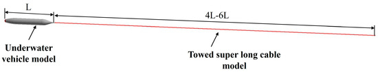
Figure 1.
Simplified model of underwater vehicle-towing cable system.
3. Numerical Methods and Grids
3.1. Grids and Freestream Conditions
The underwater vehicle grid model is shown in Figure 2, and its computational grid is formed by rotating the meridian section, with approximately 25 million grid numbers. The towed cable was searched using the immersion boundary method, with a control point count of approximately 1.05 million (for 4 L case) and 1.57 million (for 6 L case). It was searched in the flow direction area at the rear of the underwater vehicle, and the towed cable structure grid is shown in the red part of Figure 2. The freestream velocities in this calculation are 9.26 m/s (18 kts), 7.72 m/s (15 kts), and 5.14 m/s (10 kts), respectively, and the corresponding Reynolds numbers per unit length are , , and . The water density is 998 kg/m3, and the kinematic viscosity coefficient is m2/s.
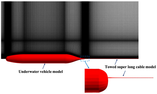
Figure 2.
Grid model of the underwater vehicle-towing cable system and its local enlarged view. The red part shows the models.
3.2. Numerical Methods
3.2.1. Flow Calculation
For the fluid calculation around the towed platform and towed cable model, based on Euler grid discretization, the three-dimensional incompressible Navier-Stokes equations are numerically solved to simulate the flow fields around the towed platform and towed cable model. To evaluate the inviscid fluxes, the Roe scheme is employed, and its accuracy is improved using the third-order MUSCL scheme with the Van Albada flux limiter, while the viscous terms are calculated using the second-order central differencing scheme. The viscous flux in the equation is discretized using the second-order central scheme, and the time progression is carried out using the LU-SGS scheme. Moreover, initial conditions in the calculations are set to the free stream values, and non-slip and adiabatic conditions are applied to the wall surface of the towing platform. The inlet boundary of the calculation area is assigned flow parameters, and the outlet boundary is treated with extrapolation.
It should be noted that a simple immersed boundary method is applied to compute the boundary of the three-dimensional towed cable. The boundary conditions of the towed cable are treated using the approach presented by Ochi et al. [25] and developed by Miyoshi et al. [18,19] and Xue et al. [20,21,22] for the study of fluid-structure interaction problems under high Reynolds number conditions, e.g., flexible subsonic and supersonic parachutes. This immersion boundary method is different from the traditional “immersion boundary method” [16], which is limited by low Reynolds numbers due to the addition of a force source term into the flow field control equation. The present simple immersion boundary method did not introduce a force source term in the control equation, which can approximately give the velocity vectors of the virtual cells where the immersed boundary is located. In this study, this method is modified so as to deal with the boundary conditions of the towed cable. The velocity vectors of the virtual cells can be obtained from the relationship between the fluid and virtual cells [21] (see Figure 3), as in Equation (1):
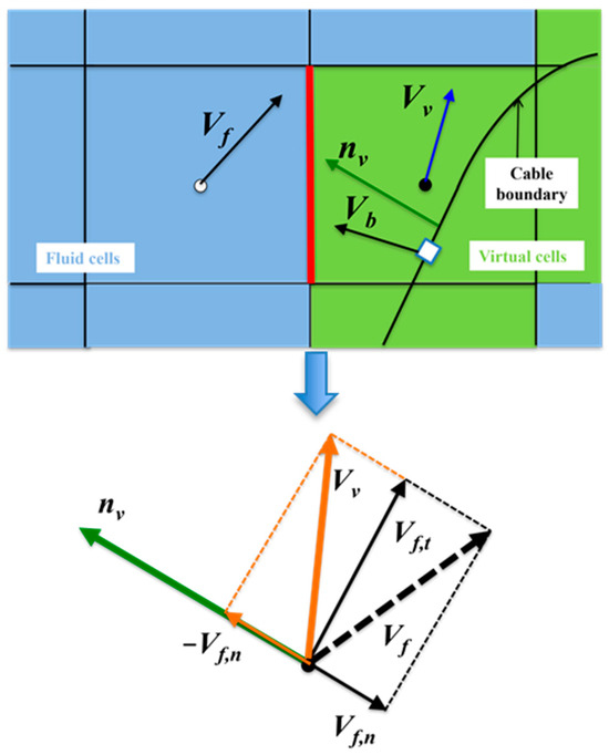
Figure 3.
The relationship between the velocity of fluid grids and virtual grids [21,22].
Here,, , and are the velocities of fluid units, virtual units, and structural nodes, and are the tangential and normal components of the fluid unit velocity, and is the unit normal vectors of the structure surface. Here, due to the huge grid numbers and the challenge of IBM in the present study, the cable is assumed to be rigid as a first step, so is equal to zero. The flexible towing super long cable will be further studied in the next step. The detailed derivation process of this equation is referred to in reference [18,21,22].
3.2.2. Structural Calculations
For the towed cable system, the coupling treatment of the fluid calculation and the solid calculation of the towed cable needs to be carried out. The towed cable is described based on the Lagrangian point, and its structural calculation uses the mass-spring-damping model to simulate the structural dynamics of the towed cable. In this model, the towed cable structure is treated as a combination of mass, spring, and damping. Based on Newton’s second law acting on each control point of the towed cable, its control equation [21] is:
Here, , , and represents the spring coefficient and the damping coefficient in the tangential and normal directions, respectively. represents the variation of the spring, represents the unit vector of adjacent mass nodes, represents the velocity of the mass node, and represents the normal vector indicated by the structure. , and respectively represent the pressure difference around the structure, gravity, tensile force of the linked structure, and inertial hydrodynamic force (Daromber force). It should be noted here that for typical quality nodes, K = 4, and for end quality nodes, K = 3. The explicit 2-order Runge Kutta scheme is used for the time progression of the towed cable structure calculations.
It should be noted that there are some impacts of rigid assumption on flow noise prediction and possible departure from true behaviors, such as: (a) eliminates flow-induced cable vibrations that typically amplify tonal noise through lock-in phenomena; (b) removes the modulation effect of cable oscillation on vortex shedding frequencies; and (c) omits strumming noise from cross-flow oscillations and friction-induced acoustic emissions at constraint points. However, the rigid cable modeling allows us to isolate the hydrodynamic noise generation mechanisms (e.g., vortex shedding, turbulent pressure fluctuations) without FSI-induced complexity, obtain benchmark data for future flexible cable comparisons, and avoid numerical instabilities from extreme geometric ratios during initial method adaptation. This staged approach enables systematic identification of noise contributors while managing computational complexity, particularly critical given the cable’s extreme slenderness induces unique numerical challenges distinct from parachute systems [20,21,22]. The subsequent phases will progressively introduce: (a) quasi-static cable reconfiguration, (b) linear elastic vibration coupling, and (c) fully-coupled nonlinear FSI in the future study.
3.2.3. Fluid-Structure-Acoustic Coupling Scheme
In a fluid-structure coupling calculation, the pressure distribution on the surface of the towed cable is used as the fluid force, which is applied to the displacement and velocity calculation of each control point of the towed cable. Then, these calculation results are used as boundary conditions and transmitted to the surrounding flow field calculation through the coupling method of immersion boundary method. In order to simultaneously calculate the fluid and structure, the weak coupling method is applied to this calculation. At each time step (N) of the calculation, the control point information obtained from the structural calculation (when N = 0, the initial model of the towed cable structure) is transferred to the flow field calculation of that calculation step (N), and the weak coupling method causes the flow field force obtained from the flow field calculation to be used for the structural calculation of the next time step (N + 1). Then, the calculation enters the next iteration as the time steps increase. In order to simultaneously and robustly calculate fluid and structure, the weak coupling method [20,21,22] was applied to this calculation.
In the final step of the calculation, the pressure pulsation obtained through fluid-structure coupling calculation is substituted into the calculation of sound pressure level (in dB), and the calculation equation is as follows:
Here, represents the effective value of pulsating sound pressure obtained from the calculation, with a reference pressure of Pa in the water medium.
3.3. Validation of Numerical Methods
In the previous studies of our team, Miyoshi et al. [18,19] used these numerical methods including the simple immersed boundary technique and the flow and structure calculation methods to simulate the flow fields around flexible parachutes at low subsonic Mach numbers (Ma = 0.06, freestream velocity is 20 m/s, Reynolds number is 2 × 10⁵), where the simulation results (i.e., the inflation time of canopy and the payload forces) for the temporal evolution of the canopy inflation agree with their experimental observations. Xue et al. [20,21,22] then used this technique to simulate flexible parachute systems at supersonic and high Reynolds number conditions, the simulation results were consistent with the results of supersonic parachute behavior during wind tunnel and flight tests (Mach numbers are 2.0, 2.2, 2.5, respectively; Reynolds numbers are from 2.0~2.5 × 10⁵, 1.0~1.2 × 10⁶, respectively) [26]. Moreover, this technique was further employed to numerically simulate the effects of the extremely slender suspension lines [20] on the flow fields around a rigid supersonic parachute, where the suspension-line shocks are generated on these lines and cause visible density disturbances, which agrees with the experimental findings obtained by NASA (Mach numbers are 2.0, 2.2, 2.5, Reynolds numbers are from 0.77~1.29 × 10⁵) [27,28]. Thus, the simple immersed boundary method and the flow and structure calculation methods used in the above simulations are also applied for the underwater vehicle and its towed cable system model in this study. Accordingly, a similar grid density is also employed for all of the cases in the present study.
4. Results and Discussions
4.1. Models with Different Cable Lengths at Different Freestream Velocities
4.1.1. Flow Field Analysis
Figure 4 shows the velocity distribution around an underwater vehicle with its 4 L and 6 L towed cable system model at 15 kts (7.72 m/s) and 18 kts (9.26 m/s). It can be observed that the towed cable has a relatively small impact on the velocity distribution at the tail of the system, and the overall velocity distribution around the towed cable is similar and less affected by changes in length and freestream flow velocity.
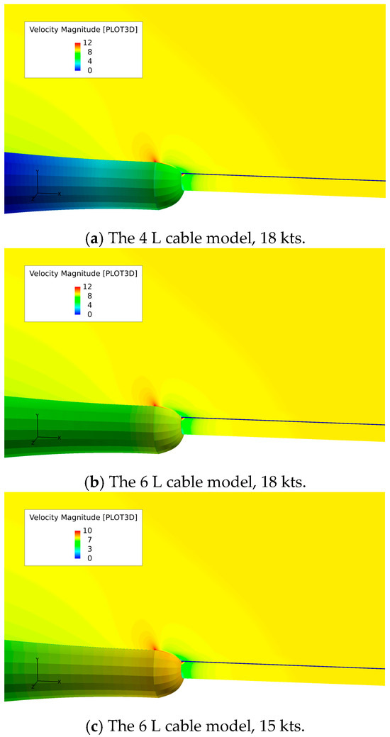
Figure 4.
Velocity contours of 4 L and 6 L towed cable models at 15 kts and 18 kts, respectively. The unit is m/s here. The color on the vehicle wall surface represents the pressure distribution.
Figure 5 shows an enlarged view of the velocity and flow direction around the cable connection part with the vehicle. From the figure, it can be observed that water flowing downstream from the vehicle appears to flow laterally under the obstruction of the cable, flowing to the left and right sides. The length of the cable has little effect on lateral flow, but a decrease in freestream flow velocity weakens the surrounding lateral flow. In Figure 6, it can be further observed that there is a local increase in velocity near the wall of the towing vehicle due to the vortex flow and lateral flow (near the cable). In the downstream flow about 0.2 mm from the rear wall, it was observed that the cable would radiate and affect the velocity distribution around it, thereby affecting the pressure pulsation changes around it. However, this impact is more pronounced in the wake region and gradually weakens further downstream.
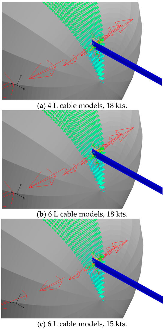
Figure 5.
Velocity vector diagrams around the 4 L and 6 L cable models at 15 and 18 kts. The velocity color is consistent with that of Figure 4.
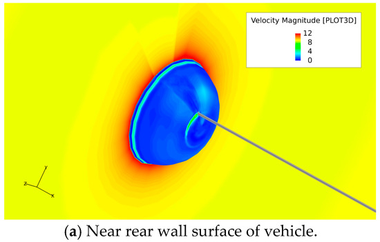
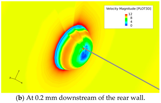
Figure 6.
Velocity distribution diagram of typical surfaces for the case of the 4 L cable model. The unit is m/s here.
4.1.2. Flow Noise Analysis
Due to the length of the towed cable, in order to analyze the pressure pulsation around the cable model and the flow noise in its vicinity, three points were taken at the top, middle, and bottom of the rear wall of the underwater vehicle. The near, middle, and far points were taken along the length direction of the towed cable model to observe the variation of its sound pressure level (SPL). From Figure 7, it can be observed that for the 6 L cable model, under the freestream condition of 18 kts, the flow noise gradually increases from top to bottom (center) along the rear wall and decreases gradually along the length direction of the towed cable. Compared with Figure 8, as the freestream velocity decreases, the variation pattern of flow noise in the two regions is consistent, but the sound pressure level decreases.
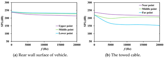
Figure 7.
SPL values at different typical points of a 6 L cable model at 18 kts.
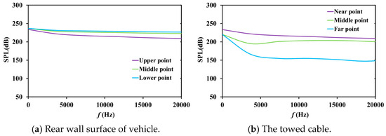
Figure 8.
SPL values of a 6 L cable model at 15 kts.
Figure 9, Figure 10 and Figure 11 show the flow noise results of the 4 L cable model at different freestream velocities. Compared with the 6 L cable model, the sound pressure level (SPL) on the rear wall of the vehicle is basically the same at 18 kts, but the length of the towed cable decreases, resulting in a significant decrease in sound pressure level at the far point. As the freestream speed decreases, the noise reduction caused by changes in cable length is consistent. It can be seen that compared to the freestream velocity, the impact of length variation is more significant.
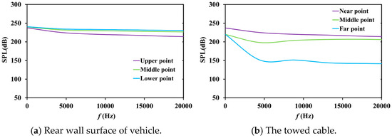
Figure 9.
SPL values of a 4 L cable model at 18 kts.
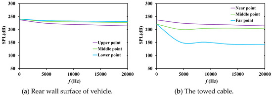
Figure 10.
SPL values of a 4 L cable model at 15 kts.
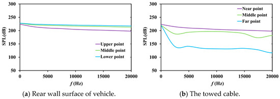
Figure 11.
SPL values of a 4 L cable model at 10 kts.
Based on the analysis of the above flow field results, it can be inferred that the longer cables (6 L) enable thicker boundary layer growth and increase vortex shedding coherence length, causing larger velocity and pressure disturbances and slower dissipation along the cable length. This explains the bigger SPL for the longer cable. In addition, longitudinal pressure gradients create cumulative flow separation effects. This explains the SPL reduction along the cable’s length, particularly at the far point where destructive interference between upstream-generated vortices and cable-end reflections occurs. Higher velocities (18 kts) enhanced turbulent kinetic energy and also intensified both pressure fluctuations and noise radiation, accordingly increasing the SPL.
4.2. Models with Different Connection Positions of Towed Cable
4.2.1. Flow Field Analysis
The 4 L cable model and the towing vehicle system at 15 kts are chosen to further investigate the influence of the connection position of the towed cable model to the underwater vehicle on its flow field distribution and flow noise, where three positions were set up along the rear wall surface of the underwater vehicle (see Figure 1) from top to bottom, as shown in Figure 12. Figure 12a–c sequentially shows the connection positions between the towed cable and the towing vehicle located near the top of the rear surface, in the middle of the surface, and near the center of the rear surface, respectively. From the comparison among Figure 12a–c, it can be found that when the cable is connected with the towing vehicle from top to middle, the cable has little impact on the velocity distribution in the wake region of underwater vehicle; however, the impact becomes most significant when the cable is connected near the center of rear wall surface.
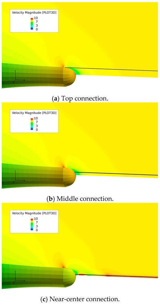
Figure 12.
Velocity distribution diagram around the towed cable when connecting at different connection positions at 15 kts. The unit is m/s here.
Figure 13 shows an enlarged view of the velocity vectors and flow direction around the towed cable connection positions. From the figure, it can be observed that the downstream flow from the real wall of vehicle is disturbed by the towed cable, and it flows laterally to the left and right sides. When the cable is connected at the top, the cable basically has little effect on the flow from upstream; when the cable is connected in the middle, there is a relatively weak lateral flow around the cable; when the cable is connected near the center, there is extremely strong lateral flow around the cable, which significantly affects the velocity distribution near the rear wall surface of the vehicle and around the towed cable, its significant impacts on the velocity distribution can also be seen from Figure 12 and Figure 14. It is worth noting that in Figure 14, it can be seen that when the cable is connected near the center position, the flow velocity near the rear wall increases sharply, which is a huge difference compared to other positions. The reasons for the larger velocity are: (1) although the wake axis is inherently a low-velocity zone (due to viscous dissipation and energy loss). However, disturbances from the cable structures disrupt the wake symmetry, inducing transverse flows (lateral velocity components, as shown in Figure 13). The disturbance generates transverse vortices, which can transport high-momentum fluid (from the mainstream or adjacent high-speed regions into the wake core. This transverse momentum injection “replenishes” the low-speed wake core, leading to a localized velocity increase. (2) The wake region typically features a low-pressure zone (due to flow separation), and disturbances may alter the local pressure distribution. The cable structures can trigger local flow reattachment, creating a favorable pressure gradient (see Figure 15c), thereby accelerating the fluid.
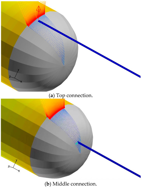
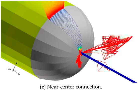
Figure 13.
The instantaneous velocity vectors around the towed cable at different connection positions at 15 kts. The velocity color is consistent with that of Figure 12.
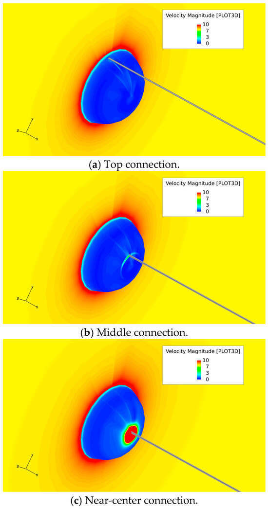
Figure 14.
Velocity distribution diagram of the near-rear wall surface at different connection positions at 15 kts. The unit is m/s here.
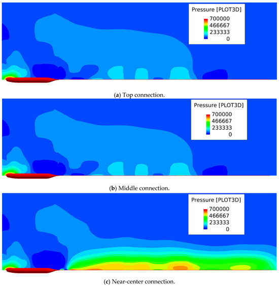
Figure 15.
Pressure distribution diagram of the downstream area of the towed cable model at different connection positions at 15 kts. The unit is Pa here.
Figure 15 shows the pressure distribution in the downstream flow at different connection positions of the towed cable and the towing vehicle. It can be observed that the cable connection position has a significant impact on the downstream area. Along the length direction of the towed cable, the pressure distribution is significantly uneven, indicating a significant pressure pulsation around the cable, which in turn generates the flow noise. From the comparison among the connection position cases, it can be seen that when the cable is connected to the upper and middle parts, the pressure distribution difference is relatively small, and when the cable is connected to the near-center position, it can be seen that the pressure distribution is extremely uneven, with a huge difference in time compared to the upper and middle parts.
4.2.2. Flow Noise Analysis
Due to the huge length of the towed cable, the flow field distribution and pressure pulsation around the cable model at different connection positions are observed from the above results, and their corresponding generating flow noise will be analyzed in the following. Figure 10, Figure 16 and Figure 17 show the variations in sound pressure levels (SPL) at six points with frequency: the upper, middle, and lower points on the rear wall surface of the underwater vehicle and the near, middle, and far points along the length direction of the towed cable model. From Figure 16, it can be observed that for the towed cable model with a length of 4 L, under the freestream condition of 15 kts, when the cable system is connected at the top position, the flow noise gradually increases from top to bottom (center) along the rear wall surface and decreases along the length direction of the towed cable. Especially at the far point, the decrease in sound pressure level is particularly significant.
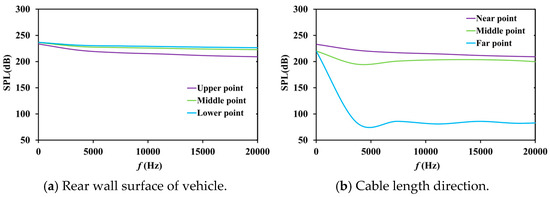
Figure 16.
SPL values of connecting cables at the top of the rear wall.
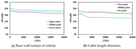
Figure 17.
SPL values of connecting cables near the center of rear wall.
Further comparing Figure 10, Figure 16 and Figure 17, it can be observed that the variation pattern of flow noise from top to center along the rear wall surface is consistent, and all gradually increase. Along the length direction of the cable, the sound pressure level changes consistently for the top and middle of the connection position of cable model, i.e., gradually decreasing from near to far points. However, when connecting the cable system in the middle of the rear wall, the sound pressure level at the far point is about 75 dB higher than that when connecting to the top of the rear wall. In addition, when connected near the center of the rear wall, the flow noise will not change monotonically and present a complex trend. The sound pressure level at the middle point along the length direction of cable is higher than that the near point along the same direction in the high-frequency range (about 5 kHz–20 kHz), and there is a significant increase change, which is totally different from that of the middle point for the top and middle connections. It should also be noted that connecting the cable system near the center point can cause a significant increase in the sound pressure level of the towed vehicle tail wall, especially in the central area, which is about 20 dB higher. This indicates that connecting the cable system near the center not only greatly disturbs the flow field distribution, velocity distribution, and pressure pulsation, but also significantly increases and complicates the flow noise.
Based on the analysis of the above flow field results, it can be explained that the cable’s longitudinal position relative to the vehicle’s wake field creates varying impedance conditions. Upper and middle connection positions of the cable relatively undisturbed flow, allowing more organized vortex shedding (lower pulsations), while central placements immerse in the vehicle’s turbulent wake, causing random pressure fluctuations through wake-cable interactions. This intensified vorticity production explains the greater pressure differentials observed in central connection cases. In addition, the connection position modifies the effective hydrodynamic diameter: central connections increase the projected cross-section in high-velocity regions of the vehicle’s wake, amplifying both turbulent kinetic energy production (via increased velocity gradients) and noise radiation from unsteady surface pressures.
5. Conclusions
In this paper, according to the structural characteristics of the towed vehicle and its towed cable model, an immersed boundary method and fluid-structure coupling method are developed. Systematic analyses of cable length, connection position, and towing speed (10–18 kts) were conducted in detail. The simulated results can be concluded as follows:
- (1)
- Unlike traditional IBM approaches limited to low-Re flows, the present developed IBM approach avoids artificial force terms and enables accurate velocity/pressure reconstruction near complex moving boundaries. This is critical for resolving the complex flow field structures and pressure fluctuations for the high-speed towed systems, in which systematic investigation of cable connection positions (top, middle, rear-center) and their impact on transverse flows, pressure pulsations, and flow noise (e.g., 20 dB increase in SPL at rear-center connections). Furthermore, the developed IBM-based approach resolves the slender geometries and adaptive resolution by decoupling grid structure from cable geometry and obtained the pressure fluctuations with noise propagation by the strong fluid-structure coupling framework.
- (2)
- The cable models with different lengths at different freestream velocities have a relatively small impact on the velocity distribution at the rear wall of the system, but there are lateral flow near the cables, which will radiate and affect the velocity distribution around them, thereby affecting the pressure pulsation changes around them and causing significant flow noise problems. Compared to the free stream flow velocity, the impact of cable length variation on flow noise is more significant.
- (3)
- When the towed cable is connected to the towing vehicle from the top to the middle, the cable has little impacts on the velocity distribution in the downstream flow of vehicle, but the impact becomes much significant when the cable is connected near the center of rear surface, where there is a very strong transverse flow around the cable, causing a sharp increase in the velocity near the rear wall.
- (4)
- When connecting the cable system with the towing vehicle, the pressure distribution in the downstream area of the platform is uneven along the cable length direction, indicating significant pressure pulsation around the cable, which in turn generates flow noise. When the cable is connected to the near center position, the uneven pressure distribution intensifies.
- (5)
- When connecting the cable system with the towing vehicle, the sound pressure level at the vehicle rear wall gradually increases from top to bottom (center) along the wall, especially when the connection position is near the center, which cause the sound pressure level near the center to be about 20 dB higher than other connection positions. Along the length direction of the cable, the sound pressure level changes consistently at the top and middle of the connection position, gradually decreasing from the near point to the far one. However, the SPL value at the far point of the middle case is about 75 dB higher than that in the top connecting. In addition, when connected near the center of the rear wall, the SPL value at the middle point is greater than that at the near point in the high-frequency range (about 5–20 kHz) and much greater than at the top and middle connections.
Overall, these results provide actionable insights for optimizing sonar array deployment (e.g., avoiding rear-center connections to minimize SPL). The longer cable increased vortex shedding coherence length, causing larger SPL. The higher velocity enhanced turbulent kinetic energy and stronger pressure gradients, leading to a larger SPL. The central placements significantly disturbed the vehicle’s turbulent wake, causing random pressure fluctuations and, accordingly, the larger SPL. Future numerical investigations will further explore the flow-structure interaction problems of the towing cables using this “immersed boundary technique” to investigate the mechanism of low-frequency flow noise caused by turbulent boundary layer on the surface of high-speed towed line arrays and flow-induced vibration of super long cables and improve the prediction ability of flow noise amplitude and phase. In addition, future efforts will focus on subsea applications, requiring collaboration with ocean engineering groups. Finally, in ongoing work, we are developing an enhanced model that incorporates both cable elasticity and full six-degree-of-freedom vehicle dynamics. This extended framework will explicitly account for the torque effects induced by off-center cable forces, enabling proper investigation of vehicle rotation and inclination phenomena.
Author Contributions
Conceptualization, X.X. and L.Q.; Methodology, Y.Y., D.Z., D.Y. and L.Q.; Formal analysis, X.X.; Investigation, X.X., D.Z. and D.Y.; Data curation, X.X., Y.Y. and L.Q.; Writing—original draft, X.X.; Writing—review & editing, L.Q.; Supervision, Y.Y., D.Z., D.Y. and L.Q. All authors have read and agreed to the published version of the manuscript.
Funding
This work was substantially supported by the National Natural Science Foundation of China (Grant No. 12072377) and the Natural Science Foundation of Hunan Province, China (Grant No. 2022JJ30678). This work was also partly supported by the Laboratory of Aerospace Entry, Descent and Landing Technology (Grant No. EDL19092309).
Data Availability Statement
Data is contained within the article.
Conflicts of Interest
The authors declare no conflict of interest.
References
- Sharif, M.B.; Ghassemi, H.; He, G.; Karimirad, M. A Review of the Flow-Induced Vibrations (FIV) In Marine Circular Cylinder (MCC) Fitted with Various Suppression Devices. Ocean Eng. 2023, 289, 116261. [Google Scholar] [CrossRef]
- Qi, L.; Zou, M.; Lin, C.; Yu, Y.; Liu, S. Directivity and Measurement of Propeller-Shaft-Hull Coupled Acoustic Radiation. Ocean Eng. 2020, 205, 107327. [Google Scholar] [CrossRef]
- Deng, D.; Huang, G.; Lou, L. Numerical Calculation of Towed Array Shape and Attitude. Ocean Eng. 1999, 1, 17–26. (In Chinese) [Google Scholar]
- Zhu, J.; Liu, J.; Deng, Z. Tower Cable Array System Simulations on Turning Manoeuvers. J. Ship Mech. 2003, 7, 33–38. (In Chinese) [Google Scholar]
- Zeng, G.; Zhu, J.; Ge, Y. Predicting the Position and Analyzing the Parameters of a Towed Array During the Maneuvering of a Submarine. J. Harbin Eng. Univ. 2009, 30, 723–727. (In Chinese) [Google Scholar]
- Dong, Y. Study on Single Towed Line Array Shape Estimation and Port/Starboard Rapid Discrimination. Master’s Thesis, Harbin Engineering University, Harbin, China, 2013. (In Chinese). [Google Scholar]
- Beerens, S.P.; IJsselmuide, S.P. Nature and Causes of Flow-Induced Noise on A Sonar with Towed Triplet Array Receiver. NAG Ned. Akoestisch Genoot. J. 2002, 161, 27–37. [Google Scholar]
- Yang, K.; Yang, Q.; Xiao, P.; Li, X.; Duan, R.; Ma, Y. Flow Noise Calculation and Experimental Study for Hydrophones in Fluid-Filled Towed Arrays. Acoust. Aust. 2017, 45, 313–324. [Google Scholar] [CrossRef]
- Howard, B.E. Calculation of The Shape of a Towed Underwater Acoustic Array. IEEE J. Ocean. Eng. 1992, 17, 193–2013. [Google Scholar] [CrossRef]
- Ablow, C.M.; Schechter, S. Numerical Simulation of Undersea Cable Dynamics. Ocean Eng. 1983, 10, 443–457. [Google Scholar] [CrossRef]
- Ma, Y.; Luan, Y.; Xu, W. Hydrodynamic Features of Three Equally Spaced, Long Flexible Cylinders Undergoing Flow-Induced Vibration. Eur. J. Mech.-B/Fluids 2020, 79, 386–400. [Google Scholar] [CrossRef]
- Huera-Huarte, F.J.; Bangash, Z.A.; González, L.M. Towing Tank Experiments on The Vortex-Induced Vibrations of Low Mass Ratio Long Flexible Cylinders. J. Fluids Struct. 2014, 48, 81–92. [Google Scholar] [CrossRef]
- Wang, F.; Ding, W.; Deng, D.; Wu, X. Motion Modeling and Numerical Simulation Study of Underwater Multi-Cable Multi-Body Towed System. J. Shanghai JiaoTong Univ. 2020, 54, 441–450. [Google Scholar]
- Wu, J.; Yang, X.; Xu, S.; Han, X. Numerical Investigation on Underwater Towed System Dynamics Using a Novel Hydrodynamic Model. Ocean Eng. 2022, 247, 110632. [Google Scholar] [CrossRef]
- Peskin, C.S. Flow Patterns Around Heart Valves: A Numerical Method. J. Comput. Phys. 1972, 10, 252–271. [Google Scholar] [CrossRef]
- Yang, F.; Gu, X.; Xia, X.; Zhang, Q. A Peridynamics-Immersed Boundary-Lattice Boltzmann Method for Fluid-Structure Interaction Analysis. Ocean Eng. 2022, 264, 112528. [Google Scholar] [CrossRef]
- Cai, Y. Study on the Numerical Modeling Methods for Underwater Fluid-Structure-Acoustic Wave Interaction Problems Based on Lattice Boltzmann Method. Ph.D. Thesis, Dalian University of Technology, Dalian, China, 2019. (In Chinese). [Google Scholar]
- Miyoshi, T.; Ishii, T.; Hashimoto, A.; Mori, K.; Nakamura, Y. Computational Analysis of Parachute Motion Using the Immersed Boundary Method. In Proceedings of the 46th AIAA Aerospace Sciences Meeting and Exhibit, Reno, NV, USA, 7–10 January 2008. [Google Scholar]
- Miyoshi, M.; Mori, K.; Nakamura, Y. Numerical Simulation of Parachute Inflation Process by IB Method. J. Jpn. Soc. Aeronaut. Space Sci. 2009, 5, 419–425. (In Japanese) [Google Scholar]
- Xue, X.P.; Koyama, H.; Nakamura, Y.; Wen, C.Y. Effects of Suspension Line on Flow Field Around a Supersonic Parachute. Aerosp. Sci. Technol. 2015, 43, 63–77. [Google Scholar] [CrossRef]
- Xue, X.P.; Nakamura, Y.; Mori, K.; Wen, C.Y.; Jia, H. Numerical Investigation of Effects of Angle-Of-Attack on A Parachute-Like Two-Body System. Aerosp. Sci. Technol. 2017, 69, 370–386. [Google Scholar] [CrossRef]
- Xue, X.P.; Nakamura, Y. Numerical Simulation of a Three-Dimensional Flexible Parachute System Under Supersonic Conditions. Trans. JSASS Aerosp. Technol. Jpn. 2013, 11, 99–108. [Google Scholar] [CrossRef]
- Jia, H.; Bao, W.; Rong, W.; Yu, L.; Xue, X.; Fan, J. Numerical Study on Aerodynamic Characteristics of Parachute Models for Future Jupiter Exploration. Space Sci. Technol. 2024, 4, 0116. [Google Scholar] [CrossRef]
- Zhang, N. Research on Mechanism and Hybrid Computation Approach for Cavity Flow and Flow Induced Noise. Ph.D. Thesis, China Ship Scientific Research Center, Wuxi, China, 2010. (In Chinese). [Google Scholar]
- Ochi, A.; Nakamura, Y. A Development of Aerodynamics Analysis Tool Using Cartesian System (First Report). In Proceedings of the Japan Society of Fluid Mechanics 19th CFD Symposium, Tokyo, Japan, 13–15 December 2005. (In Japanese). [Google Scholar]
- Sengupta, A. Fluid Structure Interaction of Parachutes in Supersonic Planetary Entry. In Proceedings of the 21st AIAA Aerodynamic Decelerator Systems Technology Conference and Seminar, Dublin, Ireland, 23–26 May 2011. [Google Scholar]
- Sengupta, A.; Steltzner, A.; Witkowski, A.; Candler, G.; Pantano, C. Findings from the Supersonic Qualification Program of the Mars Science Laboratory Parachute System. In Proceedings of the 20th AIAA Aerodynamic Decelerator Systems Technology Conference and Seminar, Seattle, DC, USA, 4–7 May 2009. [Google Scholar]
- Sengupta, A.; Kelsch, R.; Roeder, J.; Wernet, M.; Witkowski, A.; Kandis, M. Supersonic Performance of Disk-Gap-Band Parachutes Constrained to A 0-Degree Trim Angle. J. Spacecr. Rocket. 2009, 46, 1155–1163. [Google Scholar] [CrossRef]
Disclaimer/Publisher’s Note: The statements, opinions and data contained in all publications are solely those of the individual author(s) and contributor(s) and not of MDPI and/or the editor(s). MDPI and/or the editor(s) disclaim responsibility for any injury to people or property resulting from any ideas, methods, instructions or products referred to in the content. |
© 2025 by the authors. Licensee MDPI, Basel, Switzerland. This article is an open access article distributed under the terms and conditions of the Creative Commons Attribution (CC BY) license (https://creativecommons.org/licenses/by/4.0/).