Convex Optimization-Based Adaptive Neural Network Control for Unmanned Surface Vehicles Considering Moving Obstacles

Abstract

This article addresses the challenge of designing obstacle avoidance control strategies for unmanned ship systems operating in environments with moving obstacles and unmodeled dynamics. First, we utilize an enhanced artificial potential field method to generate real-time paths that allow unmanned ships to avoid obstacles effectively, overcoming the design challenges posed by moving obstacles. Next, we incorporate convex optimization techniques to create a novel adaptive neural network control strategy aimed at tackling potential dynamic uncertainties in unmanned ship systems. Finally, we present simulation results that demonstrate the effectiveness of the proposed dynamic obstacle avoidance control strategy.

1. Introduction

The application of unmanned surface vehicles (USVs) has become increasingly widespread in recent years. Compared to traditional manned systems, USVs offer significant advantages in maritime rescue and ocean exploration. However, it is important to recognize that obstacles are unavoidable along unmanned navigation routes. As the missions of unmanned ships become more complex, the need for effective obstacle avoidance capabilities is growing. Therefore, research into obstacle avoidance control for USVs is essential for ensuring their safe navigation. In recent years, research on obstacle avoidance control for USVs has attracted the attention of many scholars [1,2,3,4,5,6].

Unmanned surface vehicles (USVs) play a crucial role in maritime applications, necessitating advanced guidance and control strategies to ensure efficient and safe navigation. To address the challenges of target tracking in the presence of obstacles, Du et al. [7] propose a bias proportional guidance law incorporating a look angle constraint, enabling the USV to maintain proper orientation toward the target at the final time. In environments with static or dynamic obstacles, a hierarchical control scheme is introduced by Ahiska et al. [8] to enhance USV maneuverability and collision avoidance capabilities. Furthermore, Wen et al. [9] develop a distributed model predictive control (MPC)-based framework for robust collision avoidance and formation navigation in multi-USV systems. A domain protection task between two adversarial groups of autonomous surface vehicles (ASVs) is studied in [10], where a neurodynamics-based attack-defense guidance method is proposed for defending ASVs to achieve the collision-free capture of attacking ASVs, and by experimental results, the effectiveness of the proposed method in securing the protected domain is validated.

It can be concluded from the above work that combining a predefined obstacle avoidance path with a line-of-sight (LOS)-based control strategy provides a feasible method for addressing the problem of static obstacles. However, the challenge of obstacle avoidance for moving objects is significantly more complex. The development of obstacle avoidance control strategies for unmanned vessels navigating around moving obstacles requires further enhancement, primarily due to the lack of detailed information on avoidance paths in advance. Obstacles like floating marine debris and moving buoys are often not marked on navigation charts, leading to ineffective avoidance strategies based on traditional offline path planning. Furthermore, moving obstacles typically possess inherent speeds. For instance, the sudden appearance of a ship can also be considered an obstacle. As ships become more autonomous, the difficulty of obstacle avoidance control tends to increase. The real-time changes in the position and velocity of obstacles make it challenging to generate avoidance paths offline, further complicating the control of obstacle avoidance systems.

On the other hand, adaptive and intelligent control approaches are widely utilized to address the inherent uncertainties in USV systems [11,12,13,14,15,16,17]. These methods enhance system robustness and adaptability, enabling USVs to operate effectively in dynamic and uncertain maritime environments. The autonomous control of underactuated surface vessels faces challenges such as input saturation, unmodeled dynamics, and marine disturbances. To address these issues, Qin et al. [18] propose an adaptive finite-time event-triggered control (AFETC) that integrates an auxiliary dynamic system, adaptive techniques, and an event-triggered mechanism to enhance stability. Li et al. [19] introduce a Gaussian Process-based Extended Kalman Filter (GP-EKF) within a Learning Model Predictive Control (LMPC) framework, reducing measurement noise and improving control performance. Park et al. [20] develop an output feedback control law using neural networks to estimate unmeasured states while handling input saturation and underactuation, ensuring trajectory tracking. These advancements contribute to more effective and adaptive control strategies for USVs in complex marine environments. A robust three-dimensional (3D) path-following control framework for underactuated autonomous underwater vehicles (AUVs) subject to internal and external uncertainties is proposed in [21]. The framework employs a 3D guidance controller for path-following stability and a heuristic adaptive fuzzy algorithm with a feedback linearization PID controller to handle nonlinear dynamics and system uncertainties. The proposed method reduces the complexity of traditional dynamic controllers and mitigates dependence on precise system modeling. In [22], a human-in-the-loop coordinated path-following (HCPF) control method is proposed to address the challenge of path following for marine vehicles (MVs) in the presence of sudden disturbances caused by moving obstacles (MOs). The method combines robust exact differentiator (RED) observers, output feedback continuous twisting control (OFCTC) laws, a path updating mechanism, and a human-in-the-loop virtual leader to enable safe and synchronized path following. In [23], a composite learning control scheme is proposed for the trajectory tracking of underactuated autonomous underwater vehicles (AUVs) with unknown dynamics and time-varying disturbances. The method uses the line-of-sight (LOS) approach for underactuation and compensates for uncertainties through composite learning, incorporating both prediction and tracking errors for improved adaptation. An event-triggered asymptotic tracking control scheme for underactuated ships is proposed in [24]. It employs hyperbolic tangent functions for tracking, RBF NNs for uncertainty approximation, and MLP for computational efficiency. Variable-threshold triggering reduces communication traffic, ensuring stable control. However, the above control methods often require detailed signals of obstacle avoidance paths or relevant parameters of dynamic models, which may not be suitable for obstacle avoidance control scenarios involving moving obstacles. At present, there are few research results on moving obstacle avoidance control for unmanned ship systems with uncertain dynamics.

In this paper, we design a convex optimization-based adaptive neural controller for uncertain USVs that are considering moving obstacles. Firstly, we use the artificial potential field-dynamical virtual ship method to obtain obstacle avoidance paths in real-time, effectively overcoming the challenges posed by moving obstacles. Then, based on convex optimization techniques, we design an adaptive fuzzy strategy to overcome the uncertainty of USVs. Finally, we provide a simulation case to demonstrate the effectiveness of the proposed method.

The structures of this article are as follows: Section 2 introduces the control model and defines the control objectives. Section 3 introduces the design of obstacle avoidance algorithm and controller and analyzes its performance. Section 4 provides a detailed simulation analysis to prove the effectiveness of the proposed method. Section 5 concludes the article.

2. Problem Description

Dynamic Model of Unmanned Surface Vehicles

The nonlinear dynamics of the USVs is provided as [25]

$$\begin{array}{cc}\hfill \tau & =M\dot{v}+C\left(v\right)v+D\left(v\right)v\hfill \end{array}$$

(1)

$$\begin{array}{cc}\hfill \dot{\eta }& =J\left(\eta \right)v\hfill \end{array}$$

(2)

where M is the inertia matrix, $C\left(v\right)$ is the Coriolis matrix, $D\left(v\right)$ denotes the drag matrix, and $J\left(\eta \right)$ is the transformation matrix. The detailed information about M, C, D and J is given by

$$\begin{array}{c}\hfill M=\left[\begin{array}{ccc}m-X_{\dot{u}}& 0& -m{y}_G\\ 0& m-Y_{\dot{v}}& m{x}_G-Y_{\dot{r}}\\ -m{y}_G& m{x}_G-N_{\dot{v}}& I_z-N_{\dot{r}}\end{array}\right]\end{array}$$

(3)

$$\begin{array}{c}\hfill C\left(v\right)=\left[\begin{array}{ccc}0& 0& -m(x_{G}r+v)\\ 0& 0& -m(y_{G}r-u)\\ m(x_{G}r+v)& m(y_{G}r-u)& 0\end{array}\right]\\ \hfill +\left[\begin{array}{ccc}0& 0& 2(Y_{\dot{v}}v+\left({\displaystyle \frac{Y_{\dot{r}}+N_{\dot{v}}}{2}}\right)r)\\ 0& 0& -X_{\dot{u}}u\\ 2(-Y_{\dot{v}}v-\left({\displaystyle \frac{Y_{\dot{r}}+N_{\dot{v}}}{2}}\right)r)& X_{\dot{u}}u& 0\end{array}\right]\end{array}$$

(4)

$$\begin{array}{c}\hfill \begin{array}{c}D\left(v\right)=-\left[\begin{array}{ccc}{X}_u& 0& 0\\ 0& Y_v& Y_r\\ 0& N_v& N_r\end{array}\right]\hfill \\ -\left[\begin{array}{ccc}{X}_{u\left|u\right|}\left|u\right|& 0& 0\\ 0& Y_{v\left|v\right|}\left|v\right|+Y_{v\left|r\right|}\left|r\right|& Y_{r\left|v\right|}\left|v\right|+Y_{r\left|r\right|}\left|r\right|\\ 0& N_{v\left|v\right|}\left|v\right|+N_{v\left|r\right|}\left|r\right|& N_{r\left|v\right|}\left|v\right|+N_{r\left|r\right|}\left|r\right|\end{array}\right]\hfill \end{array}\end{array}$$

(5)

$$\begin{array}{c}\hfill J\left(\eta \right)=\left[\begin{array}{ccc}cos\psi & -sin\psi & 0\\ sin\psi & cos\psi & 0\\ 0& 0& 1\end{array}\right]\end{array}$$

(6)

where $x_G$ and $y_G$ are the center of gravity, $X_u$, $Y_v$, $Y_r$, $N_v$, and $N_r$ are the linear damping coefficients, and $X_{\dot{u}}$, $Y_{\dot{v}}$, $Y_{\dot{r}}$, $N_{\dot{v}}$, and $N_{\dot{r}}$ represent the hydrodynamic added masses. $Y_{v\left|v\right|}$, $Y_{v\left|r\right|}$, $Y_{r\left|v\right|}$, $Y_{r\left|r\right|}$, $N_{v\left|v\right|}$, $N_{v\left|r\right|}$, $N_{r\left|v\right|}$, and $N_{r\left|r\right|}$ are the maneuvering coefficients, and $X_{u\left|u\right|}$ is the resistance and current coefficient.

By neglecting the non-diagonal terms in the inertia and drag matrices, the 3-DOF mathematical model for USVs is given by [26]

$$\begin{array}{cc}\hfill \dot{x}& =ucos\left(\psi \right)-vsin\left(\psi \right)\hfill \\ \hfill \dot{y}& =usin\left(\psi \right)+vcos\left(\psi \right)\hfill \\ \hfill \dot{\psi }& =r\hfill \\ \hfill \dot{u}& ={\displaystyle \frac{1}{m-X_{\dot{u}}}}\left[(m-Y_{\dot{v}})vr+X_{u\left|u\right|}u\left|u\right|+X_{u}u+{\tau }_u\right]\hfill \\ \hfill \dot{v}& =X_{u}r+Y_{v}v\hfill \\ \hfill \dot{r}& ={\displaystyle \frac{1}{I_z-N_{\dot{r}}}}\left[(-X_{\dot{u}}+Y_{\dot{v}})vu+N_{r\left|r\right|}r\left|r\right|+N_{r}r+{\tau }_r\right]\hfill \end{array}$$

(7)

where ${\tau }_x$ and ${\tau }_z$ denote the control signals.

In this paper, a convex optimization-based adaptive neural network control method is proposed for USVs under the condition that all the dynamic coefficiencies are unknown. A modification of the APF-DVS navigation law is developed to generate the real-time obstacle avoidance path. As a result, the USV can effectively avoid moving obstacles at a reference speed $u_d$.

Assumption 1.

For simplicity, we define obstacles as circles, and their information can be detected.

3. Design and Performance Analysis of Obstacle Avoidance Controller

In this section, we present a novel adaptive neural network control strategy for unmanned ship systems with uncertain dynamics, specifically aimed at addressing obstacle avoidance problems in the presence of moving obstacles. The section is organized into three main parts. The first part focuses on the real-time algorithm for generating obstacle avoidance paths. The second part outlines the adaptive neural network control strategy for the velocity subsystem. Finally, the third part details the design process of the adaptive neural network controller for the angle subsystem.

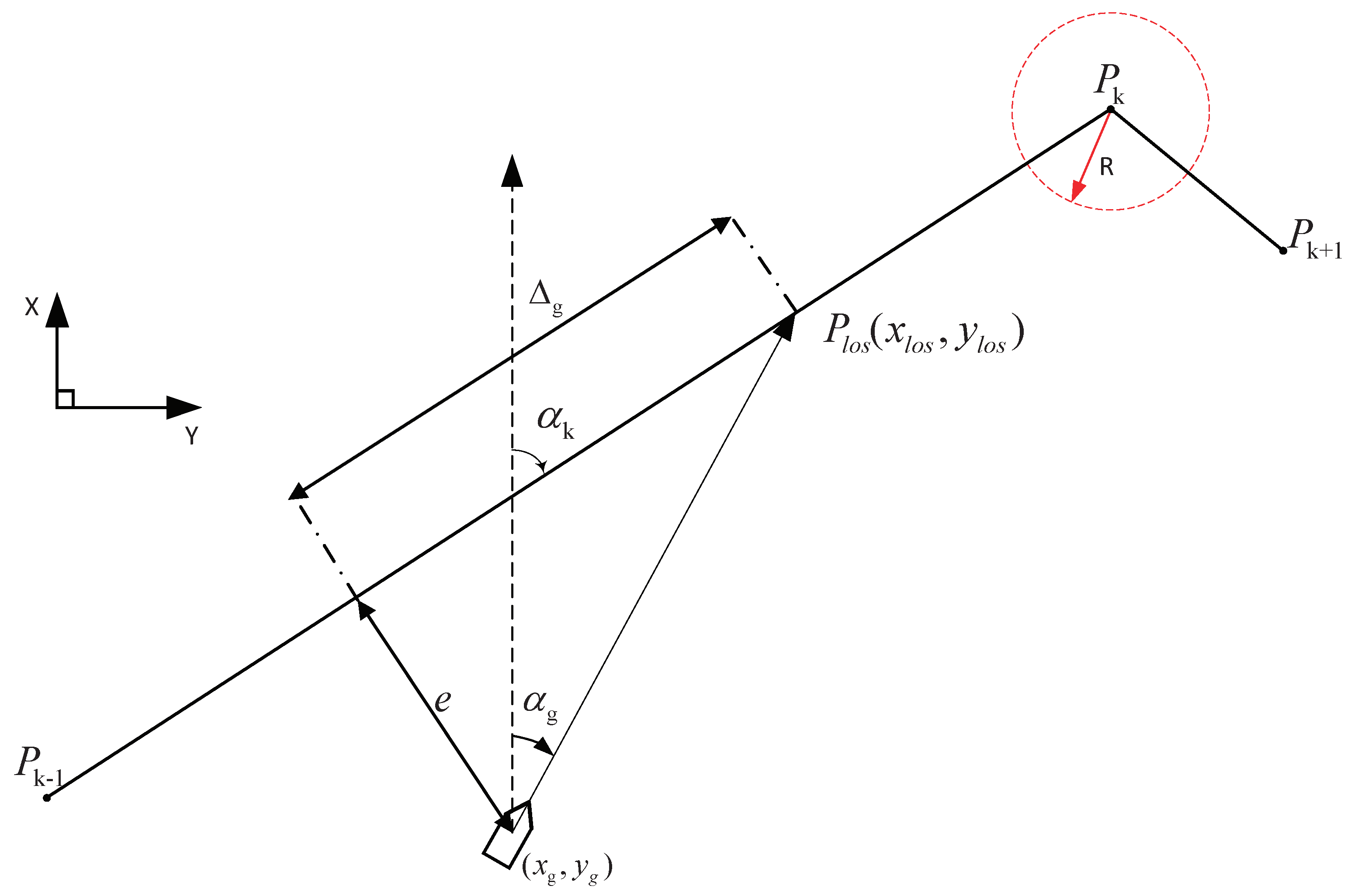
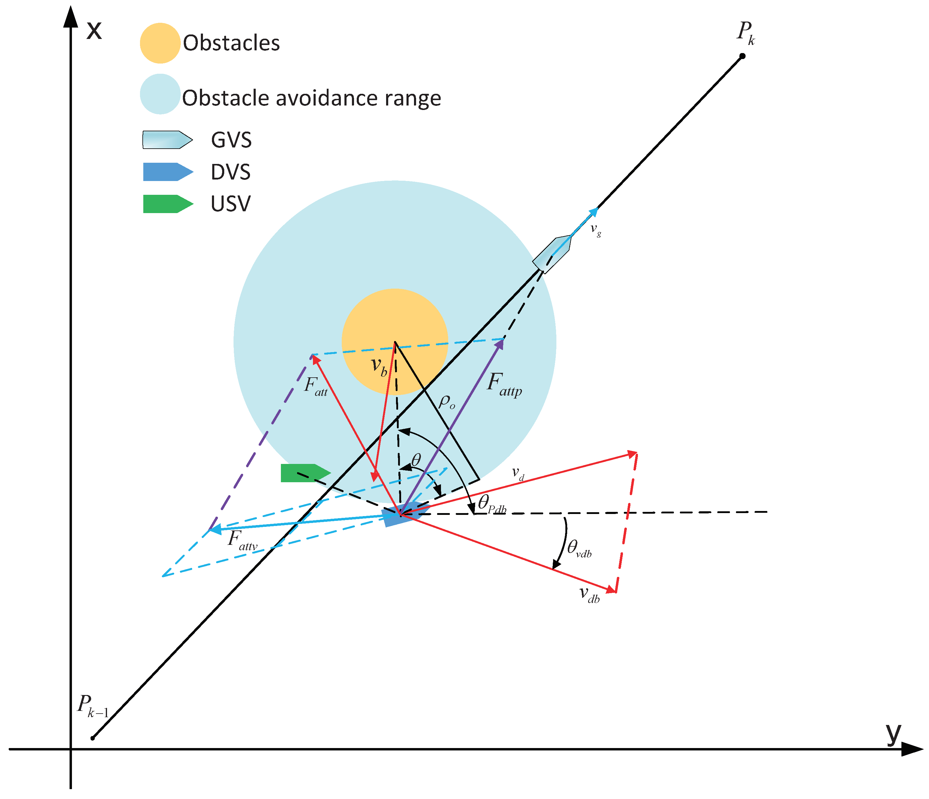
3.1. Real-Time Obstacle Avoidance Path Generation Algorithm

In this section, we propose a novel navigation method designed to address the real-time generation of obstacle avoidance paths for unmanned ships navigating around moving obstacles. Our navigation strategy involves three components [27,28]: guidance virtual ship (GVS), dynamical virtual ship (DVS), and unmanned surface vehicle (USV). The GVS generates smooth guidance paths based on the given waypoints, while the DVS follows GVS and creates real-time paths for obstacle avoidance. By coordinating these systems, we can effectively steer the USV to follow the paths generated by the GVS, thereby avoiding moving obstacles.

In our navigation method, the movement of GVS does not need to consider the influence of obstacles. Thus, the speed of GVS is directly set to the reference speed. And the line-of-sight (LOS) algorithm is a common guiding principle in the scene of straight-line path-following mission and can be used to generate the smooth curve for GVS as shown in Figure 1 [29]. $P_{k-1}$, $P_k$, and $P_{k+1}$ are path points given in advance. $P_{los}=(x_{los},y_{los})$ is the expectation point on the line segment between the past path point $P_{k-1}$ and the current path point $P_k$. The LOS guidance law for a straight line based on the visual distance is

$$\begin{array}{cc}\hfill & {\psi }_{\mathrm{g}}={\alpha }_k+arctan\left({\displaystyle \frac{-e}{{\Delta }_{\mathrm{g}}}}\right)\hfill \end{array}$$

(8)

$$\begin{array}{cc}\hfill & e=-(y_i-y_{\mathrm{g}})sin\left({\alpha }_k\right)+(x_i-x_{\mathrm{g}})cos\left({\alpha }_k\right)\hfill \end{array}$$

(9)

$$\begin{array}{cc}\hfill & {\alpha }_k=arctan{\displaystyle \frac{x_i-x_{i-1}}{y_i-y_{i-1}}}\hfill \end{array}$$

(10)

where ${\Delta }_{\mathrm{g}}=nLpp$ is the visible distance ($Lpp$ is the length of the ship). e is defined as the distance between the GVS gravity center and the path, and ${\alpha }_k$ denotes the path-tangential angle. When GVS enters the range of path point $P_k$ with a radius of R, it will switch to the next target point $P_{k+1}$ [30].

We achieve the obstacle avoidance function by planning the movement path of DVS. Thus, a modified APF algorithm [31] is developed to generate the path of DVS, which is shown in Figure 2.

The definition of attractive field $U_{att}(p,v)$ is as follows:

$$\begin{array}{cc}\hfill & U_{att}(p,v)={\displaystyle \frac{k_{ap}}{2}}{\rho }_{p_{d\mathrm{g}}}^2(p_d,p_{\mathrm{g}})+{\displaystyle \frac{k_{av}}{2}}{\rho }_{v_{d\mathrm{g}}}^2(v_d,v_{\mathrm{g}})\hfill \end{array}$$

(11)

$$\begin{array}{cc}\hfill & {\rho }_{p_{d\mathrm{g}}}(p_d,p_{\mathrm{g}})=\sqrt{{(x_d-x_{\mathrm{g}})}^2+{(y_d-y_{\mathrm{g}})}^2}\hfill \end{array}$$

(12)

$$\begin{array}{cc}\hfill & {\rho }_{v_{d\mathrm{g}}}({\mathit{v}}_d,{\mathit{v}}_{\mathrm{g}})=\sqrt{{(v_{dx}-v_{\mathrm{g}x})}^2+{(v_{dy}-v_{\mathrm{g}y})}^2}\hfill \end{array}$$

(13)

where $k_{ap}$ and $k_{av}$ are positive proportional weight coefficients about the position gravitation and velocity gravitation. ${\rho }_{p_{d\mathrm{g}}}(p_d,p_{\mathrm{g}})$ is the relative distance between GVS and DVS, and ${\rho }_{v_{d\mathrm{g}}}(v_d,v_{\mathrm{g}})$ is the relative velocity of GVS to DVS. ${\mathit{p}}_d=(x_d,y_d)$ is the DVS position, and ${\mathit{v}}_d=(v_{dx},v_{dy})$ is the DVS velocity. ${\mathit{p}}_{\mathrm{g}}=(x_{\mathrm{g}},y_{\mathrm{g}})$ is the GVS position, and ${\mathit{v}}_{\mathrm{g}}=(v_{\mathrm{g}x},v_{\mathrm{g}y})$ is the GVS velocity.

By computing the negative gradient of $U_{att}(p,v)$, we obtain

$$\begin{array}{cc}\hfill {\mathit{F}}_{\mathit{att}}& ={\mathit{F}}_{\mathit{attp}}+{\mathit{F}}_{\mathit{attv}}\hfill \\ \hfill & =k_{ap}{\rho }_{p_{d\mathrm{g}}}{\overrightarrow{n}}_{p_{d\mathrm{g}}}+k_{av}{\rho }_{v_{d\mathrm{g}}}{\overrightarrow{n}}_{v_{d\mathrm{g}}}\hfill \end{array}$$

(14)

where ${\mathit{F}}_{\mathit{attp}}$ is the attractive force generated by the relative position, and ${\overrightarrow{n}}_{p_{d\mathrm{g}}}$ is the motion direction of DVS to GVS. ${\mathit{F}}_{\mathit{attv}}$ is an attractive force generated by the relative velocity, and ${\overrightarrow{n}}_{v_{d\mathrm{g}}}$ is the motion direction of GVS to DVS.

The definition of the repulsive field $U_{rep}\left(v\right)$ is

$$\begin{array}{cc}\hfill & U_{rep}(p,v)=\hfill \\ \hfill & \left\{\begin{array}{c}{\displaystyle \frac{1}{2}}{k}_{rp}{({\displaystyle \frac{1}{{\rho }_{p_{db}}}}-{\displaystyle \frac{1}{{\rho }_d}})}^2+k_{rv}∥{\mathit{v}}_{\mathit{d}}-{\mathit{v}}_{\mathit{b}}∥cos\theta ,{\rho }_{p_{db}}<{\rho }_d\hfill \\ 0others\hfill \end{array}\right.\hfill \end{array}$$

where $k_{rv}$ and $k_{rp}$ are the positive control constant, ${\rho }_{p_{db}}$ is the distance between the DVS and obstacles, ${\rho }_d$ denotes the obstacle avoidance radius, the obstacle avoidance is only when ${\rho }_{p_{db}}<{\rho }_d$, ${\mathit{v}}_d$ is the DVS velocity, ${\mathit{v}}_{\mathit{b}}$ is the speed of moving obstacles, and $\theta ={\theta }_{p_{db}}-{\theta }_{v_{db}}$, ${\theta }_{p_{db}}=arctan{\displaystyle \frac{p_{d{b}_y}}{p_{d{b}_x}}}$, and ${\theta }_{v_{db}}=arctan{\displaystyle \frac{v_{d{b}_y}}{v_{d{b}_x}}}$ represent the angles of ${\mathit{p}}_{\mathit{db}}(p_{d{b}_x},p_{d{b}_y})$ and ${\mathit{v}}_{\mathit{db}}(v_{d{b}_x},v_{d{b}_y})$, respectively.

The negative gradient of $U_{rep}(p,v)$ gives us the repulsive force $F_{\mathrm{rep}}$:

$$\begin{array}{cc}\hfill & {\mathit{F}}_{\mathbf{rep}}={\mathit{F}}_{\mathit{repp}\mathbf{1}}+{\mathit{F}}_{\mathit{repv}\mathbf{1}}+{\mathit{F}}_{\mathit{repv}\mathbf{2}}\hfill \\ \hfill & {\mathit{F}}_{\mathit{repp}\mathbf{1}}=-k_{rp}({\displaystyle \frac{1}{{\rho }_{p_{db}}}}-{\displaystyle \frac{1}{{\rho }_d}}){\displaystyle \frac{1}{{\rho }_{p_{db}}^2}}{\overrightarrow{n}}_{p_{db}}\hfill \\ \hfill & {\mathit{F}}_{\mathit{repv}\mathbf{1}}=-k_{rv}∥{\mathit{v}}_{\mathit{d}}-{\mathit{v}}_{\mathit{b}}∥sin\theta [-sin{\theta }_{p_{db}},cos{\theta }_{p_{db}}]\hfill \\ \hfill & {\mathit{F}}_{\mathit{repv}\mathbf{2}}=-k_{rv}∥{\mathit{v}}_{\mathit{d}}-{\mathit{v}}_{\mathit{b}}∥sin\theta [sin{\theta }_{v_{db}},-cos{\theta }_{v_{db}}]\hfill \end{array}$$

where ${\mathit{F}}_{\mathit{repp}\mathbf{1}}$ represents the repulsive force arising from the relative position between DVS and obstacles, ${\overrightarrow{n}}_{p_{db}}$ is the unit vector from DVS to the obstacle, ${\mathit{F}}_{\mathit{repv}\mathbf{1}}$ denotes the repulsive force perpendicular to the ${\mathit{p}}_{\mathit{db}}$ direction, and ${\mathit{F}}_{\mathit{repv}\mathbf{2}}$ signifies the repulsive force resulting from the relative velocity between the USV and obstacles. Therefore, we choose the resultant force as ${\mathit{F}}_{\mathit{total}(\mathit{x},\mathit{y})}={\mathit{F}}_{\mathit{att}}+{\mathit{F}}_{\mathit{rep}}$. According to the LOS algorithm [29], we define ${\psi }_h={\psi }_d+arctan(-ye,{\Delta }_L)-\beta$, where ${\Delta }_L$ is a positive constant and ${\psi }_d=arctan({\mathit{F}}_{total}\left(y\right)/{\mathit{F}}_{total}\left(x\right))$, $\beta =arctan(v/u)$, $ye=-(x-x_d)sin({\psi }_d+\beta )+(y-y_d)cos({\psi }_d+\beta )$.

In order to reduce the difficulty of solving ${\dot{\psi }}_h$, we introduce the following command filter:

$$\begin{array}{c}\hfill {\dot{\widehat{\psi }}}_h=-I_1({\widehat{\psi }}_h-{\psi }_h)\end{array}$$

(15)

where $I_1$ is a positive constant. The dynamic behaviors of DVS and GVS are given by

$$\begin{array}{c}\hfill \left\{\begin{array}{c}{\dot{x}}_i=u_{i}cos{\psi }_i,\hfill \\ {\dot{y}}_i=u_{i}sin{\psi }_i,i=\mathrm{g},d\hfill \end{array}\right.\end{array}$$

(16)

where $(x_{\mathrm{g}},y_{\mathrm{g}})$, $(x_d,y_d)$ represent the positions of GVS and DVS, respectively. $u_{\mathrm{g}}$ and $u_d$ are the speeds of GVS and DVS. ${\psi }_{\mathrm{g}}$ and ${\psi }_d$ denote the angles for GVS and DVS. In this paper, the value of $u_{\mathrm{g}}$ and $u_d$ is set in advance, so we just need to design ${\psi }_{\mathrm{g}}$ and ${\psi }_d$ to solve the path planning for both GVS and DVS.

3.2. Adaptive Neural Control Strategy for Forward Speed Subsystem

The purpose of this subsection is to design the control function ${\tau }_u$ to adjust the USV speed to the desired value $u_d$. The subsystem for the forward speed of the ship is

$$\begin{array}{c}\hfill \dot{u}={\displaystyle \frac{1}{m-X_{\dot{u}}}}\left[(m-Y_{\dot{v}})vr+X_{u\left|u\right|}u\left|u\right|+X_{u}u+{\tau }_u\right]\end{array}$$

(17)

Define the tracking error as

$$\begin{array}{cc}\hfill u_e& =u-u_d\hfill \end{array}$$

(18)

For the forward speed control system, we establish the following Lyapunov function:

$$\begin{array}{c}\hfill V_{u1}={\displaystyle \frac{1}{2}}{u}_e^2\end{array}$$

(19)

And then, taking the derivative of $V_{u1}$, we have

$$\begin{array}{cc}\hfill {\dot{V}}_{u1}& =(\dot{u}-{\dot{u}}_d)u_e\hfill \\ \hfill & =\{{\displaystyle \frac{1}{m-X_{\dot{u}}}}\left[(m-Y_{\dot{v}})vr+X_{u\left|u\right|}u\left|u\right|+X_{u}u+{\tau }_u\right]-{\dot{u}}_d\}{u}_e\hfill \end{array}$$

(20)

Note that the right term in (20) contains uncertain functions ${\displaystyle \frac{1}{m-X_{\dot{u}}}}$, $X_{u\left|u\right|}$ and $X_u$, which presents challenges in the controller design. Neural networks possess a strong ability to approximate these uncertain terms [32]. Therefore, the adaptive neural network forward speed controller is given by

$$\begin{array}{c}\hfill {\tau }_u=-k_1{u}_e-{\Phi }_u^T{h}_u\left(Z_u\right)\end{array}$$

(21)

where $k_1$ is a positive constant, and ${\Phi }_u^T{h}_u\left(Z_u\right)$ denotes the RBF neural network. ${\Phi }_u={[{\varphi }_{u,1},{\varphi }_{u,2},\dots ,{\varphi }_{u,N}]}^T$ is weight vector, $h_u\left(Z_u\right)={[h_{u,1}\left(Z_u\right),h_{u,2}\left(Z_u\right),\dots ,h_{u,N}\left(Z_u\right)]}^T$ is the radial basis vector, and $Z_u={[u,v,r,u_e]}^T$ is the input signals. For $i=1,2,\dots ,N$, $h_{u,i}\left(Z_u\right)$ is chosen as the radial basis function defined in the following equation:

$$\begin{array}{c}\hfill h_{u,i}\left(Z_u\right)=exp\left[{\displaystyle \frac{-{(Z_u-{\gamma }_{u,i})}^T(Z_u-{\gamma }_{u,i})}{{\xi }_{u,i}^2}}\right]\end{array}$$

(22)

where ${\gamma }_{u,i}=[{\gamma }_{u,i,1},\dots ,{\gamma }_{u,i,4}]$ is the center vector, and ${\xi }_i$ is the width of the Gaussian function. Thus, ${\dot{u}}_e$ can be written as

$$\begin{array}{c}\hfill {\dot{u}}_e={\displaystyle \frac{1}{m-X_{\dot{u}}}}\left[(m-Y_{\dot{v}})vr+X_{u\left|u\right|}u\left|u\right|+X_{u}u-k_1{u}_e-{\Phi }_u^T{h}_u\left(Z_u\right)\right]-{\dot{u}}_d\end{array}$$

(23)

To construct a neural network weight update strategy, we define the following command filter [33,34]:

$$\begin{array}{c}\hfill {\dot{\widehat{u}}}_e=-w_1({\widehat{u}}_e-u_e)\end{array}$$

(24)

where $w_1$ is a positive constant and ${ϵ}_1={\dot{u}}_e-{\dot{\widehat{u}}}_e$. Thus, we have

$$\begin{array}{cc}\hfill {\dot{\widehat{u}}}_e+{ϵ}_1=& {\displaystyle \frac{1}{m-X_{\dot{u}}}}\left[(m-Y_{\dot{v}})vr+X_{u\left|u\right|}u\left|u\right|+X_{u}u-k_1{u}_e-{\Phi }_u^T{h}_u\left(Z_u\right)\right]-{\dot{u}}_d\hfill \end{array}$$

(25)

And then we can obtain

$$\begin{array}{cc}\hfill {\dot{\widehat{u}}}_e+k_1{u}_e=& {\displaystyle \frac{1}{m-X_{\dot{u}}}}\left[(m-Y_{\dot{v}})vr+X_{u\left|u\right|}u\left|u\right|+X_{u}u-k_1{u}_e-{\Phi }_u^T{h}_u\left(Z_u\right)\right]-{\dot{u}}_d-{ϵ}_1+k_1{u}_e\hfill \end{array}$$

(26)

The above establishes the intrinsic relationship between unmodeled dynamics, system inputs, system states, and command filter output signals. Therefore, we can construct neural network adaptive laws based on this relationship.

Thus, we define the nonlinear term $F_u={\displaystyle \frac{1}{m-X_{\dot{u}}}}\left[(m-Y_{\dot{v}})vr+X_{u\left|u\right|}u\left|u\right|+X_{u}u-k_1{u}_e\right]-{\dot{u}}_d-{ϵ}_1+k_1{u}_e$ Hence, (26) is rewritten as

$$\begin{array}{cc}\hfill {\dot{\widehat{u}}}_e+k_1{u}_e=& F_u-{\displaystyle \frac{1}{m-X_{\dot{u}}}}{\Phi }_u^T{h}_u\left(Z_u\right)\hfill \end{array}$$

(27)

The above formula can be regarded as the approximation error between $F_u$ and ${\Phi }_u^T{h}_u\left(Z_u\right)$. Therefore, a convex optimization-based method is proposed to derive the adaptive law for NNs.

For the forward speed control subsystem, the cost function is defined as

$$\begin{array}{cc}\hfill J_u\left({\Phi }_u\right)& ={\displaystyle \frac{1}{2}}{(F_u-{\displaystyle \frac{1}{m-X_{\dot{u}}}}{\Phi }_u^T{h}_u\left(Z_u\right))}^2\hfill \end{array}$$

Thus, the optimization issue is described as the following minimization problem. It is assumed that the cost function $J_u$ has an ideal value ${\Phi }_u^{*}$

$$\begin{array}{c}\hfill {\Phi }_u^{*}=arg\underset{{\Phi }_u\in R^N}{min}\{\underset{Z_u\in {\Omega }_{Z_u}}{sup}|F_u-{\Phi }_u^T{h}_u\left(Z_u\right)\left|\right\}\end{array}$$

(28)

where ${\Omega }_{Z_u}$ is a compact set. It is noted that our goal is to design weight vector ${\Phi }_u$, let ${\Phi }_u\to {\Phi }_u^{*}$. Therefore, we only need to obtain

$$\begin{array}{c}\hfill \underset{{\Phi }_u\in R^N}{min}{J}_u\left({\Phi }_u\right)\end{array}$$

(29)

and thus, we have

$$\begin{array}{c}\hfill {\displaystyle \frac{\partial J_u\left({\Phi }_u\right)}{\partial {\Phi }_u}}=-(F_u-{\displaystyle \frac{1}{m-X_{\dot{u}}}}{\Phi }_u^T{h}_u\left(Z_u\right)){\displaystyle \frac{1}{m-X_{\dot{u}}}}{h}_u\left(Z_u\right)\end{array}$$

(30)

Then, we have

$$\begin{array}{c}\hfill {\displaystyle \frac{{\partial }^2{J}_u\left({\Phi }_u\right)}{\partial {\Phi }_u^2}}={\displaystyle \frac{1}{{(m-X_{\dot{u}})}^2}}{h}_u^T\left(Z_u\right)h_u\left(Z_u\right)\ge 0\end{array}$$

(31)

Therefore, $J_u\left({\Phi }_u\right)$ is a convex function with respect to ${\Phi }_u$. According to [35], we can obtain that

$$\begin{array}{c}\hfill {({\Phi }_u-{\Phi }_u^{*})}^T{\displaystyle \frac{\partial J_u\left({\Phi }_u\right)}{\partial {\Phi }_u}}\ge 0\end{array}$$

(32)

We create Lyapunov functions $V_1={\displaystyle \frac{1}{2}}{({\Phi }_u-{\Phi }_u^{*})}^T({\Phi }_u-{\Phi }_u^{*})$. We can obtain

$$\begin{array}{c}\hfill {\dot{V}}_1={({\Phi }_u-{\Phi }_u^{*})}^T{\dot{\Phi }}_u\end{array}$$

(33)

and we design the update law for the weight vector of the speed subsystem as

$$\begin{array}{cc}\hfill {\dot{\Phi }}_u& ={\eta }_u({\dot{\widehat{u}}}_e+k_1{u}_e)h_u^T\left(Z_u\right)\hfill \end{array}$$

(34)

where ${\eta }_u>0$ is a constant. Substituting (34) and (32), one has

$$\begin{array}{c}\hfill {\dot{V}}_1=-{\eta }_u{({\Phi }_u-{\Phi }_u^{*})}^T{\displaystyle \frac{\partial J_u\left({\Phi }_u\right)}{\partial {\Phi }_u}}\le 0\end{array}$$

(35)

According to the Lasalle invariant principle [36], ${\Phi }_u$ will converge to a local minima of ${\Phi }_u^{*}$. Therefore, there is a bounded error between ${\Phi }_u$ and the ideal value ${\Phi }_u^{*}$. Thus, for the cost function $J_u\left({\Phi }_u\right)$, we have the following equation:

$$\begin{array}{c}\hfill F_u={\displaystyle \frac{1}{m-X_{\dot{u}}}}{\Phi }_u^T{h}_u\left(Z_u\right)+{ϵ}_u\end{array}$$

(36)

where ${ϵ}_u$ represents the error between $F_u$ and ${\displaystyle \frac{1}{m-X_{\dot{u}}}}{\Phi }_u^T{h}_u\left(Z_u\right)$. According to (27) and (36)

$$\begin{array}{c}\hfill {\displaystyle \frac{1}{m-X_{\dot{u}}}}\left[(m-Y_{\dot{v}})vr+X_{u\left|u\right|}u\left|u\right|+X_{u}u-k_1{u}_e\right]-{ϵ}_1+k_1{u}_e={\Phi }_u^T{h}_u\left(Z_u\right)+{ϵ}_u\end{array}$$

(37)

We establish a Lyapunov function for speed subsystem

$$\begin{array}{cc}\hfill {\dot{V}}_{u1}& =\left\{{\displaystyle \frac{1}{m-X_{\dot{u}}}}\left[(m-Y_{\dot{v}})vr+X_{u\left|u\right|}u\left|u\right|+X_{u}u-k_1{u}_e-{\Phi }_u^T{h}_u\left(Z_u\right)\right]\right\}{u}_e\hfill \\ \hfill & =\{\left[F_u-{\displaystyle \frac{1}{m-X_{\dot{u}}}}{\Phi }_u^T{h}_u\left(Z_u\right)\right]+{ϵ}_1-k_1{u}_e\}{u}_e\hfill \\ \hfill & =({ϵ}_u+{ϵ}_1-k_1{u}_e)u_e\hfill \end{array}$$

(38)

According to the following Young‘s Inequality,

$$\begin{array}{cc}\hfill {ϵ}_u{u}_e\le & {\displaystyle \frac{1}{2}}{ϵ}_u^2+{\displaystyle \frac{1}{2}}{u}_e^2\hfill \end{array}$$

(39)

$$\begin{array}{cc}\hfill {ϵ}_1{u}_e\le & {\displaystyle \frac{1}{2}}{ϵ}_1^2+{\displaystyle \frac{1}{2}}{u}_e^2\hfill \end{array}$$

(40)

Thus, we can obtain

$$\begin{array}{cc}\hfill {\dot{V}}_{u1}\le & -(k_1+1)u_e^2+{\displaystyle \frac{1}{2}}{ϵ}_u^2+{\displaystyle \frac{1}{2}}{ϵ}_1^2\hfill \\ \hfill \le & -a_u{V}_{u1}+b_u\hfill \end{array}$$

(41)

where

$$\begin{array}{cc}\hfill a_u& =2k_1+2\hfill \\ \hfill b_u& ={\displaystyle \frac{1}{2}}{ϵ}_u^2+{\displaystyle \frac{1}{2}}{ϵ}_1^2\hfill \end{array}$$

(42)

Solving Equation (41), we have

$$\begin{array}{c}\hfill V_{u1}\le (V_{u1}\left(0\right)-{\displaystyle \frac{b_u}{a_u}})e^{-a_{u}t}+{\displaystyle \frac{b_u}{a_u}},t\ge 0\end{array}$$

(43)

The above formula illustrates that $li{m}_{t\to +\infty }{V}_{u1}=b_u/a_u$. Thus, we have all the control signals, and tracking errors in the forward speed control subsystem are bounded [37,38].

3.3. Adaptive Neural Control Strategy for Heading Angle Subsystem

The heading angle subsystem for the USV is given by

$$\begin{array}{cc}\hfill \dot{\psi }& =r\hfill \end{array}$$

(44)

$$\begin{array}{cc}\hfill \dot{r}& ={\displaystyle \frac{1}{I_z-N_{\dot{r}}}}\left[(-X_{\dot{u}}+Y_{\dot{v}})vu+N_{r\left|r\right|}r\left|r\right|+N_{r}r+{\tau }_z\right]\hfill \end{array}$$

(45)

We define the tracking error of the heading angle as

$$\begin{array}{c}\hfill {\psi }_e=\psi -{\widehat{\psi }}_h\end{array}$$

(46)

Taking the derivative of ${\psi }_e$, we have

$$\begin{array}{cc}\hfill {\dot{\psi }}_e& =z_1+r_v-{\dot{\widehat{\psi }}}_h\hfill \end{array}$$

(47)

where $z_1=r-r_v$ is the control error and $r_v$ is the virtual control function. Based on the backstepping method, the virtual function $r_v$ is given by

$$\begin{array}{c}\hfill r_v=-k_2{\psi }_e+{\dot{\widehat{\psi }}}_h\end{array}$$

(48)

where $k_2$ is a positive constant.

Thus, we define the following Lyapunov function:

$$\begin{array}{c}\hfill V_{z1}={\displaystyle \frac{1}{2}}{\psi }_e^2+{\displaystyle \frac{1}{2}}{z}_1^2\end{array}$$

(49)

We calculate the derivative of the above formula

$$\begin{array}{cc}\hfill {\dot{V}}_{z1}=& z_1\{{\displaystyle \frac{1}{I_z-N_{\dot{r}}}}\left[(-X_{\dot{u}}+Y_{\dot{v}})vu+N_{r\left|r\right|}r\left|r\right|+N_{r}r+{\tau }_z\right]-{\dot{r}}_v\}+{\psi }_e(z_1-k_2{\psi }_e)\hfill \end{array}$$

(50)

Similarly, in order to address the uncertain terms ${\displaystyle \frac{1}{I_z-N_{\dot{r}}}}$, $-X_{\dot{u}}+Y_{\dot{v}}$, $N_{r\left|r\right|}r\left|r\right|$, $N_r$ and ${\dot{r}}_v$, we introduce neural networks into the angle controller as follows:

$$\begin{array}{c}\hfill {\tau }_z=-k_3{z}_1-{\Phi }_z^T{h}_z\left(Z_z\right)\end{array}$$

(51)

where $k_3$ is a positive constant, ${\Phi }_z={[{\varphi }_{z,1},{\varphi }_{z,2},\dots ,{\varphi }_{z,N}]}^T$ is the weight vector, and $h_z\left(Z_z\right)={[h_{z,1}\left(Z_z\right),h_{z,2}\left(Z_z\right),\dots ,h_{z,N}\left(Z_z\right)]}^T$, $Z_z$ is the input selected as ${[u,v,\psi ,r,{\widehat{\psi }}_d]}^T$. For $i=1,2,\dots ,N$, $h_{z,i}\left(Z_z\right)$ is chosen as a Gaussian function as defined in the following equation:

$$\begin{array}{c}\hfill h_{z,i}\left(Z_z\right)=exp\left[{\displaystyle \frac{-{(Z_z-{\gamma }_{z,i})}^T(Z_z-{\gamma }_{z,i})}{{\xi }_{z,i}^2}}\right]\end{array}$$

(52)

where ${\gamma }_{z,i}=[{\gamma }_{z,i,1},\dots ,{\gamma }_{z,i,5}]$ is the center vector, and ${\xi }_{z,i}$ is the width of the Gaussian function. ${\dot{z}}_1$ can be written as

$$\begin{array}{cc}\hfill {\dot{z}}_1=& \{{\displaystyle \frac{1}{I_z-N_{\dot{r}}}}\left[(-X_{\dot{u}}+Y_{\dot{v}})vu+N_{r\left|r\right|}r\left|r\right|+N_{r}r-k_3{z}_1-{\Phi }_z^T{h}_z\left(Z_z\right)\right]-{\dot{r}}_v\}\hfill \end{array}$$

(53)

To construct a neural network weight update strategy, we define the following command filter:

$$\begin{array}{c}\hfill {\dot{\widehat{z}}}_1=-w_2({\widehat{z}}_1-z_1)\end{array}$$

(54)

where $w_2$ is a positive parameter, and the filter error is ${ϵ}_3={\dot{z}}_1-{\dot{\widehat{z}}}_1$. Thus, we can obtain

$$\begin{array}{cc}\hfill {\dot{\widehat{z}}}_1+{ϵ}_3=& \{{\displaystyle \frac{1}{I_z-N_{\dot{r}}}}\left[(-X_{\dot{u}}+Y_{\dot{v}})vu+N_{r\left|r\right|}r\left|r\right|+N_{r}r+{\tau }_z\right]-{\dot{r}}_v\}\hfill \end{array}$$

(55)

Thus, (55) is written as

$$\begin{array}{cc}\hfill {\dot{\widehat{z}}}_1+{ϵ}_3=& \{{\displaystyle \frac{1}{I_z-N_{\dot{r}}}}\left[(-X_{\dot{u}}+Y_{\dot{v}})vu+N_{r\left|r\right|}r\left|r\right|+N_{r}r-k_3{z}_1-{\Phi }_z^T{h}_z\left(Z_z\right)\right]-{\dot{r}}_v\}\hfill \end{array}$$

And then we have

$$\begin{array}{cc}\hfill {\dot{\widehat{z}}}_1+k_3{z}_1=& {\displaystyle \frac{1}{I_z-N_{\dot{r}}}}\left[(-X_{\dot{u}}+Y_{\dot{v}})vu+N_{r\left|r\right|}r\left|r\right|+N_{r}r-k_3{z}_1-{\Phi }_z^T{h}_z\left(Z_z\right)\right]-{\dot{r}}_v-{ϵ}_3+k_3{z}_1\hfill \end{array}$$

(56)

We define $F_r={\displaystyle \frac{1}{I_z-N_{\dot{r}}}}\left[(-X_{\dot{u}}+Y_{\dot{v}})vu+N_{r\left|r\right|}r\left|r\right|+N_{r}r-k_3{z}_1\right]-{\dot{r}}_v-{ϵ}_3+k_3{z}_1$, and $k_3$ is a positive constant. Thus, we have

$$\begin{array}{cc}\hfill {\dot{\widehat{z}}}_1+k_3{z}_1=& F_r-{\displaystyle \frac{1}{I_z-N_{\dot{r}}}}{\Phi }_z^T{h}_z\left(Z_z\right)\hfill \end{array}$$

(57)

Same as the speed controller update law, the angle controller adaptive law of the weight vector is given by

$$\begin{array}{cc}\hfill {\dot{\Phi }}_z=& {\eta }_z({\dot{\widehat{z}}}_1+k_3{z}_1)h_z^T\left(Z_z\right)\hfill \end{array}$$

(58)

The approximation error between $F_z$ and ${\displaystyle \frac{1}{I_z-N_{\dot{r}}}}{\Phi }_z^T{h}_z\left(Z_z\right)$ is as shown in the following equation:

$$\begin{array}{c}\hfill F_z={\displaystyle \frac{1}{I_z-N_{\dot{r}}}}{\Phi }_z^T{h}_z\left(Z_z\right)+{ϵ}_z\end{array}$$

(59)

And then we establish the following Lyapunov function:

$$\begin{array}{cc}\hfill {\dot{V}}_{z1}=& z_1\{{\displaystyle \frac{1}{I_z-N_{\dot{r}}}}\left[(-X_{\dot{u}}+Y_{\dot{v}})vu+N_{r\left|r\right|}r\left|r\right|+N_{r}r-k_3{z}_1-{\Phi }_z^T{h}_z\left(Z_z\right)\right]-{\dot{r}}_v\}+{\psi }_e(z_1-k_2{\psi }_e)\hfill \end{array}$$

(60)

and then we can obtain

$$\begin{array}{cc}\hfill {\dot{V}}_{z1}=& z_1[F_r-{\displaystyle \frac{1}{I_z-N_{\dot{r}}}}{\Phi }_z^T{h}_z\left(Z_z\right)+{ϵ}_3-k_3{z}_1]+{\psi }_e(z_1-k_2{\psi }_e)\hfill \\ \hfill =& z_1[{ϵ}_z+{ϵ}_3-k_3{z}_1]+{\psi }_e(z_1-k_2{\psi }_e)\hfill \\ \hfill =& z_1{ϵ}_z+z_1{ϵ}_3-k_3{z}_1^2+{\psi }_e{z}_1-k_2{\psi }_e^2\hfill \end{array}$$

(61)

By using the following Young’s inequality,

$$\begin{array}{c}\hfill z_1{ϵ}_z\le {\displaystyle \frac{1}{2}}{z}_1^2+{\displaystyle \frac{1}{2}}{ϵ}_z^2\\ \hfill z_1{ϵ}_3\le {\displaystyle \frac{1}{2}}{z}_1^2+{\displaystyle \frac{1}{2}}{ϵ}_3^2\\ \hfill {\psi }_e{z}_1\le {\displaystyle \frac{1}{2}}{\psi }_e^2+{\displaystyle \frac{1}{2}}{z}_1^2\end{array}$$

(62)

Thus, (61) can be written as

$$\begin{array}{cc}\hfill {\dot{V}}_{z1}\le & -(k_3+{\displaystyle \frac{3}{2}})z_1^2-(k_2+{\displaystyle \frac{1}{2}}){\psi }_e^2+{\displaystyle \frac{1}{2}}{ϵ}_3^2+{\displaystyle \frac{1}{2}}{ϵ}_z^2\hfill \\ \hfill & \le -a_z{V}_{z1}+b_z\hfill \end{array}$$

(63)

where

$$\begin{array}{c}\hfill a_z=min\{2k_3+3,2k_2+1\}\\ \hfill b_z={\displaystyle \frac{1}{2}}{ϵ}_3^2+{\displaystyle \frac{1}{2}}{ϵ}_z^2\end{array}$$

(64)

Same as the analysis of the speed subsystem,

$$\begin{array}{c}\hfill V_{z1}\le (V_{z1}\left(0\right)-{\displaystyle \frac{b_z}{a_z}})e^{-a_{z}t}+{\displaystyle \frac{b_z}{a_z}},t\ge 0\end{array}$$

(65)

Furthermore, we have $li{m}_{t\to +\infty }{V}_{z1}=b_z/a_z$.

Remark 1.

The cost functions of optimization problems $J_u$, $J_z$ are only given for the purpose of analysis. The values of such functions do not need to be calculated in our controller.

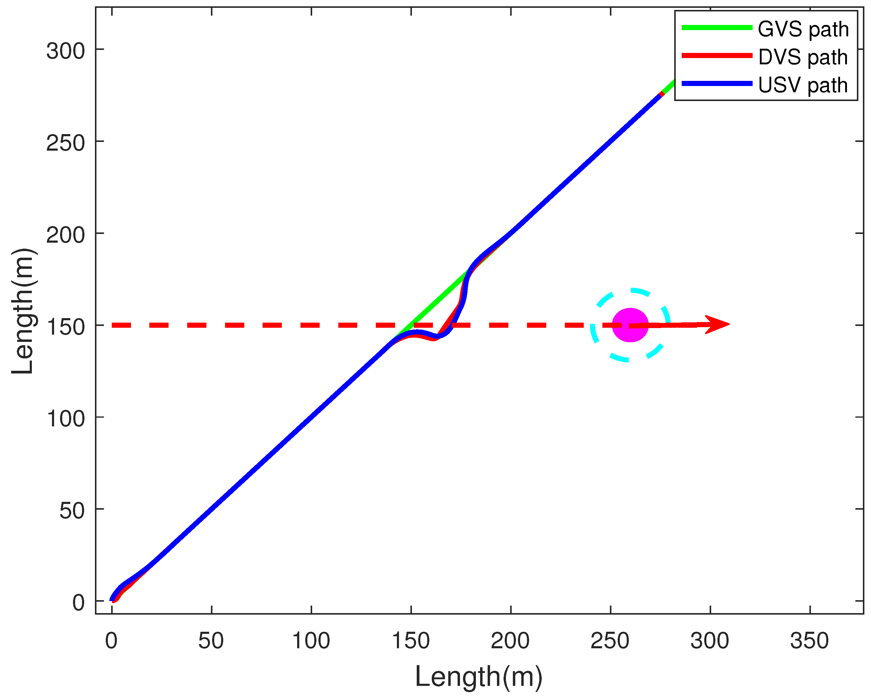
4. Simulation Results and Performance Analysis

In this section, we conduct simulation experiments to validate the feasibility of the proposed convex optimization-based intelligent controller for the USVs. The simulation model parameters we select refer to papers [25,39], and the system parameters are shown in

Table 1. USV model parameters.

$X_u$		$25,(u>1.2)64.55$
$N_r$	0.02	$-\pi \rho \sqrt{(u^2+v^2)}{T}^2{L}^2$
$X_{\dot{u}}$		−2.25
$Y_{\dot{v}}$		−23.13
$N_{\dot{r}}$		−2.79
$X_{u\left|u\right|}$		$0,(u>1.2)-70.92$
$N_{r\left|r\right|}$		−3.49

. The draft of the boat is T = 0.09, the overall length is L = 1.01, and the beam of each individual hull is 0.75.

The reference speed for the USV is set to 0.5 m/s. The endpoints of the reference path are (0,0), and (300,300), respectively. A circular obstacle with a radius of 8 m is used in the simulation. The location of the obstacle circle center is (0,150). The motion trajectory of the obstacle is described as $y=0.325$ t. Thus, the moving speed of the obstacle is $0.325$ m/s. The number of neural networks for both the speed and angle subsystems is set to three. For the neural network of the speed control subsystem, our neural network input selection is $Z_u={[u,v,r,u_e]}^T$, the center vectors are ${\gamma }_{u,1}={[0.1,0.1,0.1,0.1]}^T$, ${\gamma }_{u,2}={[0.5,0.5,0.5,0.5]}^T$, ${\gamma }_{u,3}={[0.9,0.9,0.9,0.9]}^T$, the width of the Gaussian function is ${\xi }_{u,i}=0.5$ to ensure sufficient generalization with $i=1,2,3$. The weight vector initial value is ${\Phi }_u={[0.1,0.1,0.1]}^T$. For the neural network in the angle control subsystem, the neural network input is ${[u,v,\psi ,r,{\widehat{\psi }}_h]}^T$, the center vectors are ${\gamma }_{z,1}={[0.1,0.1,0.1,0.1,0.1]}^T$, ${\gamma }_{z,2}={[0.5,0.5,0.5,0.5,0.5]}^T$, ${\gamma }_{z,3}={[0.9,0.9,0.9,0.9,0.9]}^T$, the width of the Gaussian function ${\xi }_{z,i}=0.5$, where $i=1,2,3$. And the initial value of the weight vector is ${\Phi }_z={[0.1,0.1,0.1]}^T$.

The other controller parameters are shown in

Table 2. Controller parameters and obstacle avoidance parameters.

Parameters	Value	Parameters	Value
$k_1$	30	$k_2$	20
$k_3$	30	$w_1$	0.1
$w_2$	0.1	${\eta }_u$	20
${\eta }_z$	20	$k_{ap}$	0.1
$k_{av}$	0.1	$k_{rp}$	1500
$k_{rv}$	5	$I_1$	0.1
${\Delta }_L$	10

. The initial position of our tested ship is (0,0), and the initial speed is set to 0.3. All the initial neural weights used in our controller are set to 0.1. The control flowchart is shown in Figure 3.

The simulation results are presented in Figure 4, Figure 5, Figure 6 and Figure 7. Figure 8 illustrates the global path diagram, Figure 9 displays the input curves of our controller, while Figure 10, Figure 11, Figure 12 and Figure 13 show the motion trajectory of the tested unmanned surface vehicle (USV). Figure 5 and Figure 6 display the curves of control errors for forward speed and heading angle, respectively. Additionally, Figure 7 depicts the weight curve of the neural network for the speed subsystem, and Figure 8 presents the weight curve for the angle subsystem.

As shown in Figure 4, the green line represents the path of GVS, the red line represents the path of DVS, and the blue line represents the path of USV. The simulation results indicate significant changes in the adaptive parameters and the control law curve between 380 s and 600 s, which are attributed to obstacle avoidance actions. The navigation strategy employed in this study consists of GVS and DVS. When obstacles are detected, the artificial potential field method alters the preset angle, leading to a notable change in the control torque of the angle subsystem.

We can observe that effective tracking is achieved both before and after entering the obstacle detection range. During the obstacle avoidance process, the DVS provides a path for avoiding obstacles, enabling it to effectively navigate around moving obstacles. In the time interval from 0 to 380 s, there are no obstacles present on the reference path. Consequently, both the DVS and USV can proceed along their predetermined routes. During this stage, the error and control input curves remain relatively smooth. From 380 to 500 s, an obstacle moves closer to the reference path. For instance, at time t = 430, the center of the obstacle is located at (139.75,150). Since the GVS does not incorporate obstacle avoidance strategies, it continues to follow its original path. In contrast, the DVS employs the artificial potential field method to avoid moving obstacles, allowing the USV to follow the DVS and successfully navigate around the obstacles. Figure 7 and Figure 8 illustrate the learning process of neural network weights. Figure 9 displays the behavior of the input signals. During the simulation, the forward speed remains constant, resulting in relatively gradual changes. As a consequence, the neural network within the velocity subsystem is trained quickly. In contrast, the neural network in the heading angle control subsystem behaves differently. Since the angle controller operates as a second-order system, and because obstacle avoidance primarily requires significant changes in angle, the adjustments in this subsystem are more drastic.

To further analyze the performance of the controller during obstacle avoidance, we select various paths at different stages of the obstacle avoidance process for examination. In Figure 10, we observe that as the DVS enters the obstacle avoidance zone, an obstacle avoidance maneuver is initiated. However, the sudden change in the angle of the DVS results in a minor error in the path of the USV. In Figure 11, we can see that when the DVS is far from obstacles, it starts moving towards the GVS direction. Figure 12 and Figure 13 illustrate that the guidance algorithm has successfully executed the obstacle avoidance function, while the control algorithm effectively tracks the abrupt angle changes that occur during this process. As the DVS enters the detection range of moving obstacles, it starts to change direction, and the USV also responds by implementing tracking, demonstrating commendable control performance.

Regarding the comparative analysis, since this study primarily focuses on control algorithms that address uncertain dynamics, we provide a performance evaluation of different control methods under the same obstacle avoidance strategy. We compare our approach with the radial basis function (RBF) neural network controller [40] and the simplified adaptive backstepping controller [41]. From

Table 3. Comparison of different control methods.

Control Method	${\mathit{MAE}}_{\mathit{u}}$	${\mathit{MAE}}_{\mathit{\psi }}$
Control method in this article	4.8738 × ${10}^{-4}$	4.4089 × ${10}^{-5}$
Control method in [40]	0.0036	4.9897 × ${10}^{-5}$
Control method in [41]	0.0220	0.0019

, it is evident that the use of convex optimization techniques in this paper results in higher accuracy for our control method compared to traditional adaptive or neural network-based control methods.

We conduct 50 additional simulation tests to demonstrate the superiority of our method in managing the uncertainty of unmanned ships. In these tests, the model bias is randomly set between 0% and 100%. The results of fifty simulations are shown in Figure 14 and Figure 15, where $MA{E}_u$ is the mean absolute control error for speed subsystem and $MA{E}_{\psi }$ is the mean absolute control error for the heading angle subsystem. It can be seen that the control method proposed in this article has good control performance.

5. Conclusions

This article presents an enhanced adaptive obstacle avoidance control method for unmanned ship systems. It introduces a convex optimization-based adaptive control strategy designed to address the uncertain dynamics of unmanned ships and enhance overall control performance. By following a real-time obstacle avoidance path created using the modified artificial potential field method, the approach effectively mitigates potential safety hazards posed by moving obstacles. Simulation results demonstrate that unmanned ships can successfully track the obstacle avoidance paths defined by the proposed design. In our future work, we will investigate the obstacle avoidance control problem for unmanned ships navigating around irregularly shaped obstacles. Additionally, we plan to conduct hardware-in-the-loop simulation experiments to further validate the effectiveness of our proposed control strategy.

References

1. Gonzalez-Garcia, A.; Collado-Gonzalez, I.; Cuan-Urquizo, R.; Sotelo, C.; Sotelo, D.; Castañeda, H. Path-following and lidar-based obstacle avoidance via nmpc for an autonomous surface vehicle. Ocean Eng. 2022, 266, 112900. [Google Scholar] [CrossRef]
2. Guo, B.; Guo, N.; Cen, Z. Obstacle avoidance with dynamic avoidance risk region for mobile robots in dynamic environments. IEEE Robot. Automat. Lett. 2022, 7, 5850–5857. [Google Scholar] [CrossRef]
3. Wu, H.; Zhang, H.; Feng, Y. MPC-Based Obstacle Avoidance Path Tracking Control for Distributed Drive Electric Vehicles. World Electr. Veh. J. 2022, 13, 221. [Google Scholar] [CrossRef]
4. Wei, J.; Zhang, J.; Li, H.; Xia, J.; Liu, Z. Guidance Method with Collision Avoidance Using Guiding Vector Field for Multiple Unmanned Surface Vehicles. Drones 2025, 9, 105. [Google Scholar] [CrossRef]
5. Li, Y.; Hou, P.; Cheng, C.; Wang, B. Research on Collision Avoidance Methods for Unmanned Surface Vehicles Based on Boundary Potential Field. J. Mar. Sci. Eng. 2025, 13, 88. [Google Scholar] [CrossRef]
6. Yuan, X.; Tong, C.; He, G.; Wang, H. Unmanned Vessel Collision Avoidance Algorithm by Dynamic Window Approach Based on COLREGs Considering the Effects of the Wind and Wave. J. Mar. Sci. Eng. 2023, 11, 1831. [Google Scholar] [CrossRef]
7. Du, B.; Xie, W.; Zhang, W.; Chen, H. A target tracking guidance for unmanned surface vehicles in the presence of obstacles. IEEE Trans. Intell. Transp. Syst. 2024, 25, 4102–4115. [Google Scholar] [CrossRef]
8. Ahiska, K.; Leblebicioglu, M.K. A hierarchical control scheme for trajectory tracking usvs in environments with disturbances and dynamic obstacles. IEEE Trans. Intell. Veh. 2024, 1–10. [Google Scholar] [CrossRef]
9. Wen, G.; Lam, J.; Fu, J.; Wang, S. Distributed MPC-Based Robust Collision Avoidance Formation Navigation of Constrained Multiple USVs. IEEE Trans. Intell. Veh. 2024, 9, 1804–1816. [Google Scholar] [CrossRef]
10. Kang, T.; Gu, N.; Wang, D.; Liu, L.; Hu, Q.; Peng, Z. Neurodynamics-based attack-defense guidance of autonomous surface vehicles against multiple attackers for domain protection. IEEE Trans. Ind. Electron. 2024, 71, 12655–12663. [Google Scholar] [CrossRef]
11. Shin, J.; Kwak, D.J.; Lee, Y.-i. Adaptive path-following control for an unmanned surface vessel using an identified dynamic model. IEEE/ASME Trans. Mechatron. 2017, 22, 1143–1153. [Google Scholar] [CrossRef]
12. Liu, Z.; Zhang, Y.; Yuan, C.; Luo, J. Adaptive path following control of unmanned surface vehicles considering environmental disturbances and system constraints. IEEE Trans. Syst. Man Cybern. Syst. 2021, 51, 339–353. [Google Scholar] [CrossRef]
13. Chen, L.; Cui, R.; Yang, C.; Yan, W. Adaptive neural network control of underactuated surface vessels with guaranteed transient performance: Theory and experimental results. IEEE Trans. Ind. Electron. 2020, 67, 4024–4035. [Google Scholar] [CrossRef]
14. Li, Y.; Zhao, Y.; Tong, S. Adaptive fuzzy control for heterogeneous vehicular platoon systems with collision avoidance and connectivity preservation. IEEE Trans. Fuzzy Syst. 2023, 31, 3934–3943. [Google Scholar] [CrossRef]
15. Liu, Y.; Liu, J.; Wang, Q.-G.; Yu, J. Adaptive command filtered backstepping tracking control for auvs considering model uncertainties and input saturation. IEEE Trans. Circuits Syst. II Exp. Briefs 2023, 70, 1475–1479. [Google Scholar] [CrossRef]
16. Li, Y.; Wan, J.; Wang, X.; Sun, Z.; Li, H.; Yu, Z.; Kou, L.; Li, J.; Yang, Y. Path-following control based on alos guidance law for USV. Electronics 2025, 14, 749. [Google Scholar] [CrossRef]
17. Wang, X.; Yi, H.; Xu, J.; Xu, C.; Song, L. PID Controller Based on Improved DDPG for Trajectory Tracking Control of USV. J. Mar. Sci. Eng. 2024, 12, 1771. [Google Scholar] [CrossRef]
18. Qin, J.; Du, J.; Li, J. Adaptive finite-time trajectory tracking event-triggered control scheme for underactuated surface vessels subject to input saturation. IEEE Trans. Intell. Transp. Syst. 2023, 24, 8809–8819. [Google Scholar] [CrossRef]
19. Li, F.; Li, H.; Wu, C. Gaussian process-based learning model predictive control with application to USV. IEEE Trans. Ind. Electron. 2024, 71, 16388–16397. [Google Scholar] [CrossRef]
20. Park, B.S.; Kwon, J.-W.; Kim, H. Neural network-based output feedback control for reference tracking of underactuated surface vessels. Automatica 2017, 77, 353–359. [Google Scholar] [CrossRef]
21. Xiang, X.; Yu, C.; Zhang, Q. Robust fuzzy 3d path following for autonomous underwater vehicle subject to uncertainties. Comput. Oper. Res. 2017, 84, 165–177. [Google Scholar] [CrossRef]
22. Lv, M.; Gu, N.; Wang, D.; Han, B.; Peng, Z. Human-in-the-loop coordinated path following of marine vehicles based on continuous twisting control. IEEE Trans. Ind. Inform. 2025, 21, 465–474. [Google Scholar] [CrossRef]
23. Liu, J.; Du, J. Composite learning tracking control for underactuated autonomous underwater vehicle with unknown dynamics and disturbances in three-dimension space. Appl. Ocean Res. 2021, 112, 102686. [Google Scholar] [CrossRef]
24. Deng, Y.; Zhang, Z.; Gong, M.; Ni, T. Event-triggered asymptotic tracking control of underactuated ships with prescribed performance. IEEE Trans. Intell. Transp. Syst. 2023, 24, 645–656. [Google Scholar] [CrossRef]
25. Gonzalez-Garcia, A.; Castañeda, H. Guidance and control based on adaptive sliding mode strategy for a usv subject to uncertainties. IEEE J. Ocean. Eng. 2021, 46, 1144–1154. [Google Scholar] [CrossRef]
26. Sun, C.; Liu, J.; Yu, J. Improved adaptive fuzzy control for unmanned surface vehicles with uncertain dynamics using high-power functions. Ocean Eng. 2024, 312, 119168. [Google Scholar] [CrossRef]
27. Zhang, G.; Deng, Y.; Zhang, W.; Huang, C. Novel dvs guidance and path-following control for underactuated ships in presence of multiple static and moving obstacles. Ocean Eng. 2018, 170, 100–110. [Google Scholar] [CrossRef]
28. Zhang, G.; Zhang, X. A novel dvs guidance principle and robust adaptive path-following control for underactuated ships using low frequency gain-learning. ISA Trans. 2015, 56, 75–85. [Google Scholar] [CrossRef]
29. Lekkas, A.M.; Fossen, T.I. Integral LOS path following for curved paths based on a monotone cubic hermite spline parametrization. IEEE Trans. Control Syst. Technol. 2014, 22, 2287–2301. [Google Scholar] [CrossRef]
30. Oh, S.-R.; Sun, J. Path following of underactuated marine surface vessels using line-of-sight based model predictive control. Ocean Eng. 2010, 37, 289–295. [Google Scholar] [CrossRef]
31. Zhang, G.; Han, J.; Li, J.; Zhang, X. Apf-based intelligent navigation approach for usv in presence of mixed potential directions: Guidance and control design. Ocean Eng. 2022, 260, 111972. [Google Scholar] [CrossRef]
32. Wrat, G.; Ranjan, P.; Mishra, S.K.; Jose, J.T.; Das, J. Neural network-enhanced internal leakage analysis for efficient fault detection in heavy machinery hydraulic actuator cylinders. Proc. IMechE Part C J. Mech. Control Eng. Sci. 2025, 239, 1021–1031. [Google Scholar] [CrossRef]
33. Zheng, X.; Yang, X. Command filter and universal approximator based backstepping control design for strict-feedback nonlinear systems with uncertainty. IEEE Trans. Autom. Control 2020, 65, 1310–1317. [Google Scholar] [CrossRef]
34. Liu, J.; Wang, Q.-G.; Yu, J. Convex optimization-based adaptive fuzzy control for uncertain nonlinear systems with input saturation using command filtered backstepping. IEEE Trans. Fuzzy Syst. 2023, 31, 2086–2091. [Google Scholar] [CrossRef]
35. Boyd, S. Convex Optimization; Cambridge University Press: Cambridge, UK, 2004. [Google Scholar]
36. Khalil, H.K. Adaptive output feedback control of nonlinear systems represented by input-output models. IEEE Trans. Autom. Control 1996, 41, 177–188. [Google Scholar] [CrossRef]
37. Liu, J.; Wang, Q.-G.; Yu, J. Event-triggered adaptive neural network tracking control for uncertain systems with unknown input saturation based on command filters. IEEE Trans. Neural Netw. Learn. Syst. 2024, 35, 8702–8707. [Google Scholar] [CrossRef]
38. Li, Y.; Zhang, J.; Tong, S. Fuzzy adaptive optimized leader-following formation control for second-order stochastic multiagent systems. IEEE Trans. Ind. Inform. 2022, 18, 6026–6037. [Google Scholar] [CrossRef]
39. Sonnenburg, C.R.; Woolsey, C.A. Modeling, identification, and control of an unmanned surface vehicle. J. Field Robot. 2013, 30, 371–398. [Google Scholar] [CrossRef]
40. Xu, W.; Liu, J.; Yu, J.; Han, Y. Low complexity adaptive neural network three-dimensional tracking control for autonomous underwater vehicles considering uncertain dynamics. Eng. Appl. Artif. Intell. 2025, 142, 109860. [Google Scholar] [CrossRef]
41. Liu, J.; Chen, X.; Yu, J. Simplified adaptive backstepping control for uncertain nonlinear systems with unknown input saturation and its application. Control Eng. Pract. 2023, 139, 105639. [Google Scholar] [CrossRef]
Figure 1. Line-of-sight guidance.
Jmse 13 00587 g001
Figure 2. DVS-APF algorithm.
Jmse 13 00587 g002
Figure 3. Flowchart.
Jmse 13 00587 g003
Figure 4. The avoidance trajectory.
Jmse 13 00587 g004
Figure 5. USV speed error.
Jmse 13 00587 g005
Figure 6. USV angle error.
Jmse 13 00587 g006
Figure 7. Speed neural network weights.
Jmse 13 00587 g007
Figure 8. Angle neural network weights.
Jmse 13 00587 g008
Figure 9. Curves of USV controller input.
Jmse 13 00587 g009
Figure 10. The avoidance trajectory in t = 430 s.
Jmse 13 00587 g010
Figure 11. The avoidance trajectory in t = 460 s.
Jmse 13 00587 g011
Figure 12. The avoidance trajectory in t = 500 s.
Jmse 13 00587 g012
Figure 13. The avoidance trajectory in t = 600 s.
Jmse 13 00587 g013
Figure 14. Speed control error distribution of 50 simulation results.
Jmse 13 00587 g014
Figure 15. Angle control error distribution of 50 simulation results.
Jmse 13 00587 g015