Article

Cooperative Patrol Control of Multiple Unmanned Surface Vehicles for Global Coverage

1
School of Electronic Information and Intelligent Manufacturing, Anhui Xinhua University, Hefei 230001, China
2
Hefei Local Maritime (Port and Shipping) Management Service Center, Hefei 230011, China
*
Author to whom correspondence should be addressed.
J. Mar. Sci. Eng. 2025, 13(3), 584; https://doi.org/10.3390/jmse13030584
Submission received: 19 February 2025 / Revised: 9 March 2025 / Accepted: 11 March 2025 / Published: 17 March 2025
(This article belongs to the Section Ocean Engineering)

Abstract

:
The cooperative patrol control of multiple unmanned surface vehicles (Multi-USVs) in dynamic aquatic environments presents significant challenges in global coverage efficiency and system robustness. The study proposes a cooperative patrol control algorithm for multiple unmanned surface vehicles (Multi-USVs) based on a hybrid embedded task state information model and reward reshaping techniques, addressing global coverage challenges in dynamic aquatic environments. By integrating patrol, collaboration, and obstacle information graphs, the algorithm generates kinematically feasible control actions in real time and optimizes the exploration-cooperation trade-off through a dense reward structure. Simulation results demonstrate that the algorithm achieves 99.75% coverage in a 1 km × 1 km task area, reducing completion time by 23% and 74% compared to anti-flocking and partition scanning algorithms, respectively, while maintaining collision rates between agents (CRBAA) and obstacles (CRBAO) below 0.15% and 0.5%. Compared to DDPG, SAC, and PPO frameworks, the proposed training framework (TFMUSV) achieves 28% higher rewards with 40% smaller fluctuations in later training stages. This study provides an efficient and reliable solution for autonomous monitoring and search-rescue missions in complex aquatic environments.

1. Introduction

Multi-agent cooperative patrolling tasks involve multiple agents working together within a predefined area to collect environmental data or monitor the occurrence of sudden events through continuous patrolling. One of the core challenges in this task is the multi-agent cooperative coverage control method. This method requires ensuring full coverage of the entire task area while minimizing the length of the patrolling path through efficient path planning and control strategies, thereby improving patrolling efficiency [1]. To achieve this goal, researchers have proposed various optimization-based cooperative strategies aimed at enhancing the adaptability and execution efficiency of multi-agent systems in complex environments. These strategies not only involve communication and coordination mechanisms between agents but also emphasize how to dynamically adjust patrolling routes in response to sudden situations in a changing environment [2,3].
Given the importance of this task, this paper proposes a cooperative patrol control algorithm for Multi-USVs, aimed at global coverage. The algorithm models the mission scenario using a hybrid embedded task state information model, combined with reward reshaping techniques, enabling each node in the fleet to be trained based on real-time information, thus dynamically generating optimal control commands during mission execution. This modeling approach not only enhances the cooperative patrol efficiency of the Multi-USV system in complex aquatic environments but also provides data support for subsequent cooperative search and interception tasks. Through this method, the study introduces new ideas for decision-making in dynamic environments for Multi-USV systems, with the potential to improve system performance while optimizing the utilization of computational and communication resources.

2. Related Work

There have been many achievements in the research of multi-agent area coverage control methods. Xu et al. [4,5,6] provided a systematic summary and classification of existing area coverage control strategies. They divided the current common area coverage methods into two main categories: one is online algorithms based on a known environmental map, and the other is offline algorithms for unknown environmental maps. Furthermore, based on different approaches to area decomposition, these methods can be further classified into exact-approximate cell decomposition methods and approximate cell decomposition methods. Exact-approximate cell decomposition methods ensure the efficiency and accuracy of the coverage task by precisely dividing the area units, while approximate cell decomposition methods optimize computational complexity and resource consumption, making them suitable for more complex real-world applications. This classification system provides a clear framework for the research of multi-agent area coverage control and offers a theoretical foundation for further algorithm optimization and application promotion, as shown in Figure 1.

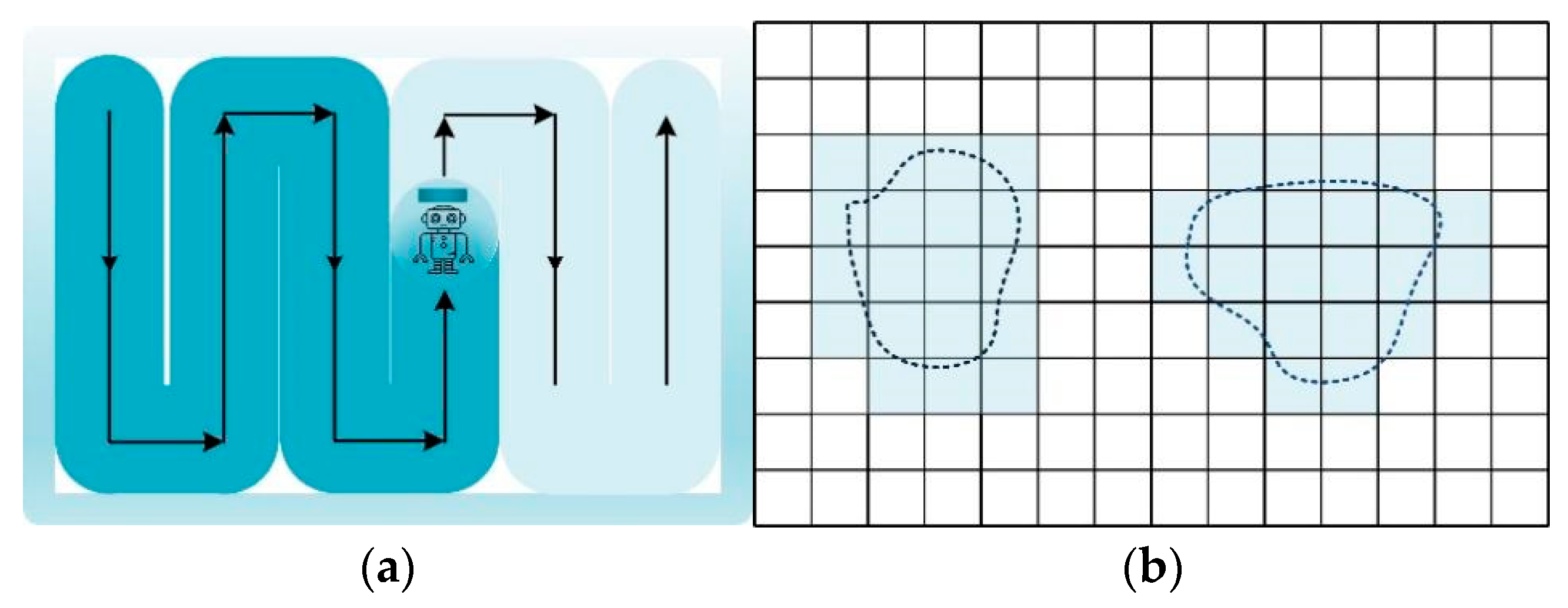
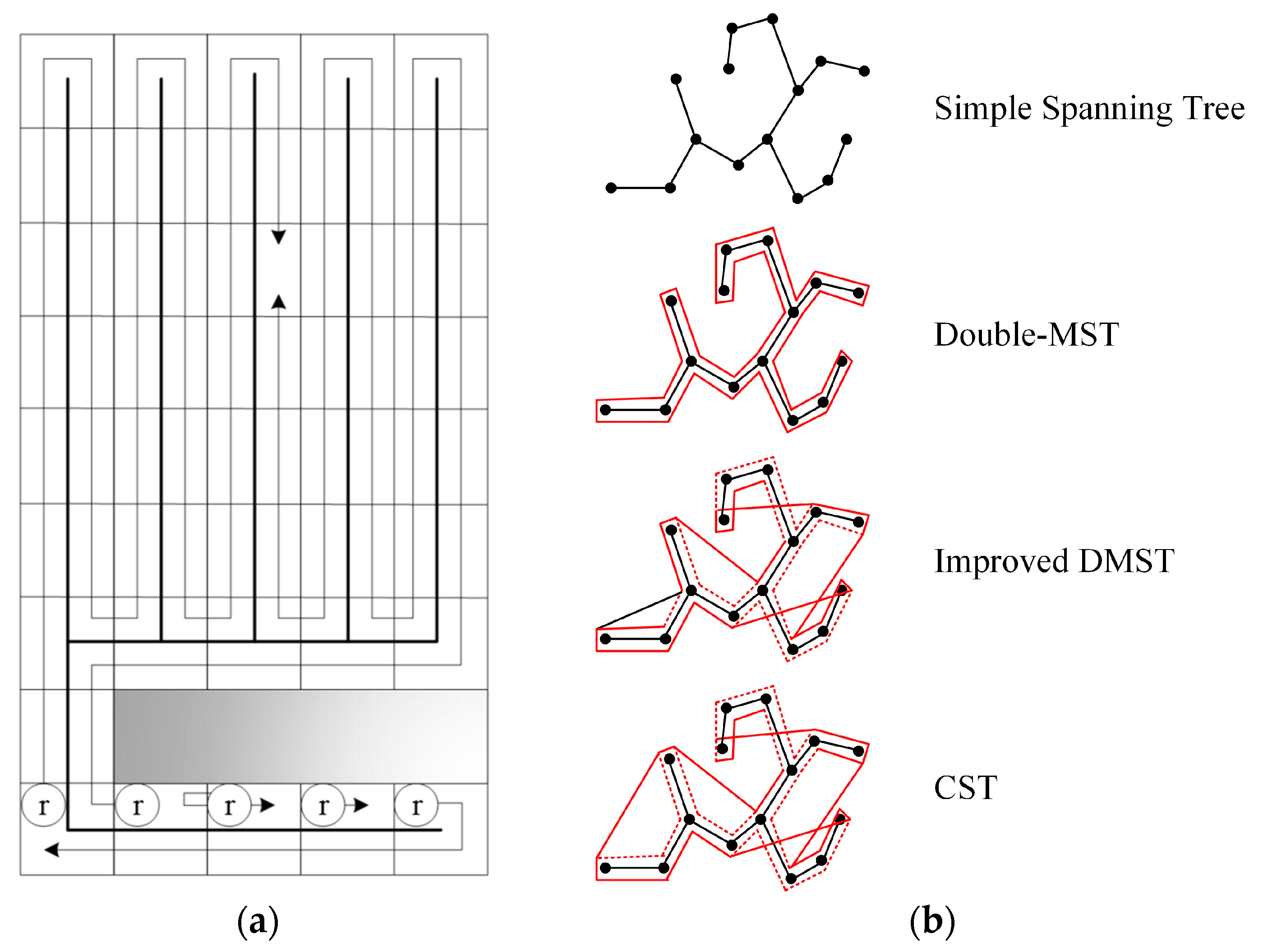
2.1. Exact-Approximate Cell Decomposition Method

The exact-approximate cell decomposition method is a method that achieves complete coverage of the entire task area by dividing it into a set of non-overlapping units. The collection of these cells is strictly equal to the free space, and there are no obstacles within them, allowing robots to use simple motion patterns for efficient coverage. Trapezoidal decomposition, plowing decomposition, and Voronoi diagram decomposition are representative techniques of exact-approximate cell decomposition, widely applied in the cooperative patrolling field of multi-agent systems, and have been extensively studied and practically validated.
In the trapezoidal decomposition method, the task area is divided into a series of trapezoidal units (as shown in Figure 2a), with each unit being covered through simple back-and-forth motion. By traversing the adjacency graph related to the decomposition, complete coverage can be ensured, ultimately generating a serrated path for the coverage units. Research on trapezoidal decomposition has been applied across multiple fields. For example, reference [7] proposed a path planning algorithm for water depth mapping that combines trapezoidal decomposition with coverage strategies, designed to generate survey paths for multiple convex regions in coastal areas, showing high reliability in practical applications. Reference [8] further explored the influence of ocean currents on the scanning direction in water depth mapping path planning, optimizing path planning by integrating the trapezoidal decomposition method. Additionally, ref. [9] proposed a coverage path planning framework for unmanned surface vehicle-assisted depth measurement, modeling the depth measurement task as an integer programming problem. This framework optimizes path length, region connectivity, and scanning direction, achieving efficient coverage through binary convex decomposition and layered heuristic algorithms. Performance advantages were validated in lake tests. Ref. [10] introduced a multi-drone flood coverage algorithm that combines deep reinforcement learning with a path dispersion strategy. By using D-infinity water flow estimation techniques to optimize path planning, the dispersion strategy prevents drone clustering in low-altitude areas. This algorithm outperforms existing methods in terms of accumulated rewards and coverage uniformity, demonstrating superior performance. These studies indicate that the trapezoidal decomposition method has immense potential in path planning and area coverage applications.
Due to the larger number of units generated by trapezoidal decomposition, multiple units may merge to form larger units, which can significantly increase the coverage path length and thus affect coverage efficiency. To address this issue, the plow-style unit decomposition method was proposed to improve path planning performance. Similar to trapezoidal decomposition, the plow-style decomposition only extends the vertices of vertical line segments (as shown in Figure 2), thus reducing the number of units and optimizing the coverage path. In related studies, Reference [11] proposed an improved Grey Wolf Algorithm for UAV path planning, optimizing flight efficiency and safety. This method accelerates convergence by dynamically adjusting the weight distribution and micro-oscillation convergence factor, enhancing the global optimum search capability. Under various constraints, this method demonstrated excellent performance, significantly improving UAV path planning efficiency and accuracy, with important application value. Reference [12] proposed an innovative UAV battery management method aimed at optimizing energy-aware task planning. By considering battery replacement requirements, this method optimizes the flight path to reduce overall flight time and avoid unnecessary long-distance flights. Reference [13] proposed a novel deep reinforcement learning method for multi-robot information path planning, aimed at mapping target areas in unknown 3D environments. The key innovation of this method is the introduction of enhanced graphs to model the trajectories of other robots, enabling communication and collision-avoidance planning between robots. Additionally, plow-style decomposition has been widely applied in UAV inspection [14] and Autonomous Underwater Vehicle (AUV) [15] fields. In path optimization, Reference [16] proposed a new meta-heuristic algorithm to solve AUV path planning problems, combining weighted center methods and fitness-based parameter selection schemes, effectively handling AUV path planning tasks in different scenarios. It also demonstrates strong adaptability in underwater environment modeling and threat modeling. Meanwhile, Reference [16] utilized an improved Sparrow Search Algorithm to plan the optimal path and combined consensus algorithms and artificial potential fields for obstacle avoidance and cooperative formation motion. Through golden search optimization and adaptive iteration methods, this approach showed strong feasibility in formation control in obstacle-rich environments. These studies fully validate the superiority and application value of the plow-style unit decomposition method in complex scenarios.
The trapezoidal decomposition and plow-style decomposition methods, by using fixed shapes (such as trapezoids or parallelograms) to partition the task area, are computationally efficient and relatively simple to implement. However, the fixed shapes of these methods limit their adaptability when dealing with complex task areas, especially those with irregular curved boundaries, multiple concave and convex parts, or non-polygonal shapes. These methods struggle to precisely align with the actual boundaries of such areas. For example, when performing mapping or coverage control in natural terrains such as mountains or rivers, these methods may result in partitioned units that do not match the actual terrain, leading to under-coverage or excessive coverage in some regions. This reduces the practical effectiveness and adaptability of the methods. To address these limitations, researchers have proposed the Voronoi diagram decomposition method, as shown in Figure 3. Based on given generator points (such as the initial positions of agents), the Voronoi diagram decomposition naturally divides the task area into multiple irregularly shaped subregions that closely match the actual shape of the area. This method overcomes the limitations of fixed shapes in trapezoidal and plow-style decompositions and is capable of handling task areas with various shapes, including convex polygons, concave polygons, and complex curved boundaries. It reduces the issues of incomplete or redundant coverage caused by decomposition methods and provides a partitioning solution that better meets the requirements of the actual environment.
Soleymani et al. [17] proposed a multi-agent area coverage control method based on the Bellman optimality framework. This approach achieves optimal tracking through an adaptive control strategy combined with actor-critic neural network reinforcement learning techniques, relying on local data rather than a global model. It was demonstrated that when agents converge to Voronoi centers, they can maximize area coverage metrics, which aligns with the solution of the Lloyd algorithm. Papatheodorou et al. [18] studied the area coverage problem for mobile robot networks with imprecise localization. Each robot has a uniform radial sensing capability and is subject to first-order kinematic constraints. This method partitions convex space based on the Voronoi principle, where each robot’s responsibility area corresponds to its Voronoi cell, with boundaries formed by hyperbolic arcs. The proposed control law is distributed and relies on the position information of its Voronoi-Delaunay “neighbors”, inherently ensuring collision avoidance. Yu et al. [19] considered uncertain kinematics and dynamics. By adopting a cost function related to the Voronoi partition, the optimal coverage control was transformed into a tracking control problem, and an adaptive dynamic and kinematic programming approach was used to design an adaptive region-optimal coverage control strategy. Magalhães et al. [20] introduced a control strategy based on Voronoi partitioning for multi-robot systems covering an environment with state and control constraints. At each moment, the Voronoi algorithm partitions the finite convex workspace, assigning each robot non-overlapping navigation areas. The partitioning is adjusted by assigning different weights to each robot, ensuring that robots with higher weights are assigned larger areas. This deployment scheme uses model predictive control and artificial vector fields to guide robots along curves toward the Chebyshev configuration centers of the Voronoi partition, ultimately stabilizing the system and achieving optimal area coverage.

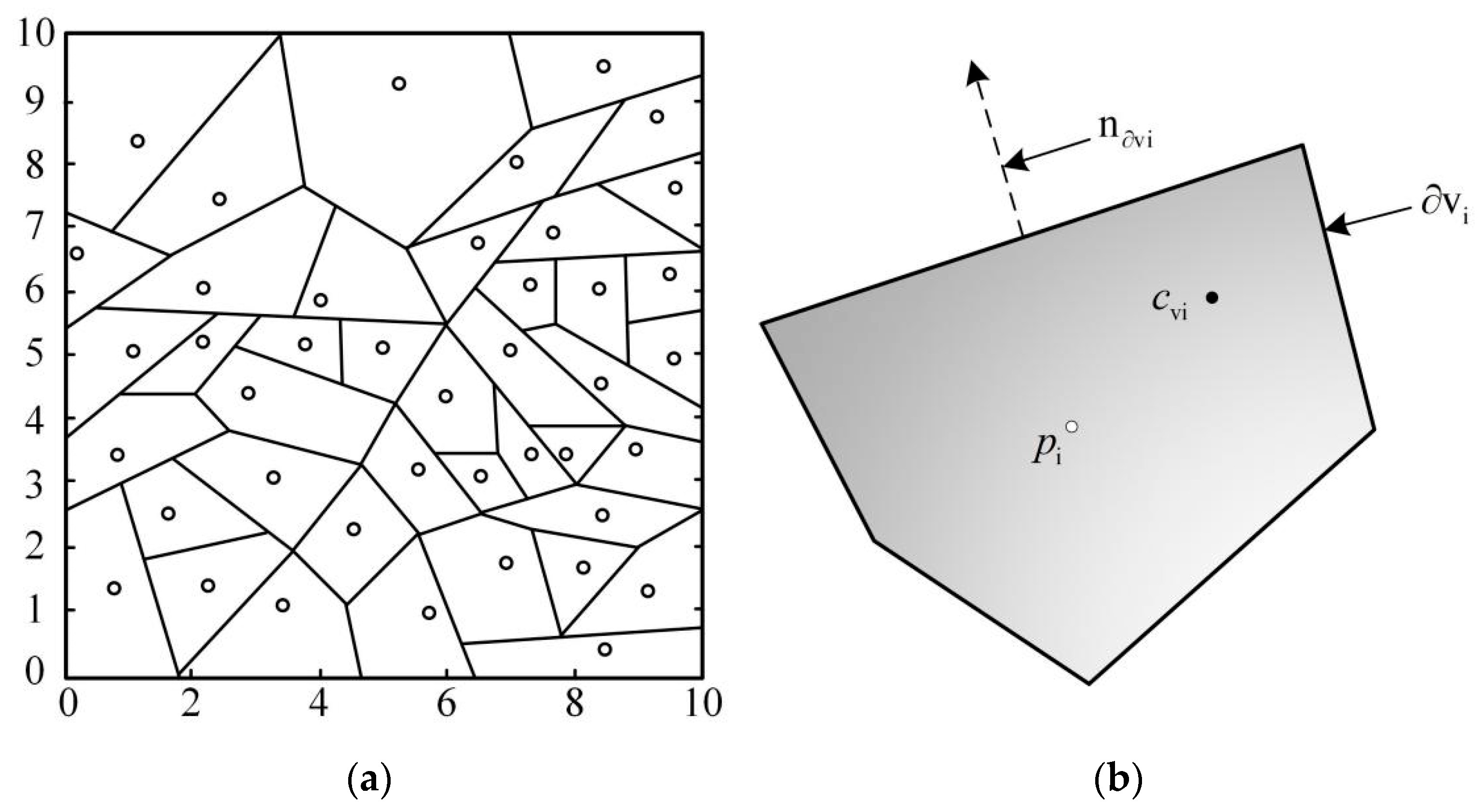
2.2. Approximate Cell Decomposition Method

The approximate cell decomposition method typically achieves effective coverage of an area by dividing the task region into cells of consistent shape and size. However, due to the presence of obstacles or boundary constraints within the task area, some cells may be discarded, meaning that the union of these cells does not fully cover the entire task area. During the partitioning process, the size of the cells is primarily determined by the detection range of the sensors equipped on the agents performing the task. Methods such as spanning tree algorithms, neural networks, and bio-inspired algorithms are typical examples of approximate cell decomposition techniques. Building on research in single-agent systems, the application of this method in multi-agent systems has also received considerable attention.
In the study of coverage in multi-agent systems, Hazon et al. [21] extended the spanning tree method to multi-robot systems using a heuristic approach, proposing the MSTC (Multi-robot Spanning Trees Coverage) method (as shown in Figure 4a). Zkahraman et al. [22] investigated the multi-objective coordination problem in robot task execution, presenting a method that combines control barrier functions with behavior trees to achieve different types of task combinations, while providing performance guarantees for task completion. This method was validated in a simulated underwater coverage task. Hyatt et al. [23] explored the problem of multi-robot online coverage path planning, which involves simultaneously performing coverage and mapping tasks in an unknown environment. They proposed an MCTS (Monte Carlo Tree Search) method based on game theory and machine learning, applying it to multi-robot online coverage path planning. The study implemented the MCTS planner and compared it with an online multi-robot planning method based on the cow-plowing algorithm under different conditions of robot numbers and obstacle densities, while also exploring the adaptability of the MCTS planner for multi-objective tasks such as minimizing turns.
Dong et al. [24] proposed an artificial weighted spanning tree covering algorithm based on the MSTC method. This approach allows each robot to independently construct a spanning tree, gravitates toward the inertia center of uncovered areas, and avoids other robots, thus balancing task distribution. It utilizes Bézier curves to optimize trajectory smoothness, improving real-time performance and dynamic consistency. This method is suitable for distributed multi-robot systems, improving coverage efficiency and enhancing robustness in patrol tasks. Xu et al. [25] proposed a complete coverage path planning algorithm for irregular areas. This method adopts adaptive pruning to optimize local paths, reduce redundancy in coverage, and decrease path complexity and theoretical energy consumption in areas with obstacles. Kim et al. [26] introduced a coverage control strategy for aerial robot formations equipped with downward-facing cameras. Based on the characteristic that camera resolution varies with height, a distributed gradient controller was designed to balance the monitoring area and perception quality, optimizing the target detection probability. Additionally, control barrier functions were used to ensure obstacle avoidance and maintain safe distances during deployment. Chen et al. [27] proposed a fast task planning framework, termed “planning decision trees”, suitable for large-scale multi-robot systems subject to temporal logic constraints. The planning decision tree incrementally constructs a tree structure to represent task progress, modeling the system state in terms of completed positions and times, thereby avoiding complex computations and reducing the search space. This method expands from the root node to the leaf nodes to meet linear temporal logic tasks, ensuring both the feasibility and completeness of the planning. Analysis shows that the solution time of the planning decision tree is linearly related to the number of robots, making it suitable for efficient task planning and offering new research ideas for autonomous coverage and patrol in multi-agent systems. Lu et al. [28] studied the path planning problem of reconfigurable modular robot systems and proposed a hybrid density network method based on obstacle perception to generate connected polygonal nodes. These nodes are then connected using convex polygon trees within a rapidly exploring random tree framework, forming candidate solutions for convex optimization problems. This method ensures connectivity, optimizes computational complexity, and improves planning efficiency in large-scale, complex environments.
In addition to the exact-approximate cell decomposition method and approximate cell decomposition method, several other approaches have also been applied to the field of multi-agent cooperative coverage control. Zhu et al. [29] and Gosrich et al. [30] proposed two coverage control methods for multi-agent systems based on graph neural networks. These methods aggregate local perceptual information from “neighbors” at different hops through the graph neural network, promoting cooperation among robots. The effectiveness of multi-communication in multi-robot coverage was verified, and the scalability and transferability of the learning-based control strategy were evaluated. Danie et al. [31] applied the ant colony optimization algorithm to optimize key parameters in a chaotic ant colony optimization mobility model. This model uses chaotic solutions based on dynamical systems and pheromones to optimize area coverage. Subsequently, genetic algorithms and coevolutionary genetic algorithms were employed to optimize the model parameters, enhancing the system’s operational capabilities. Xin et al. [32] designed a multi-robot cooperative area coverage algorithm, proposing a set of rules to divide the target coverage area into several small regions, and developed a genetic algorithm based on circular encoding to allocate these divided regions to multiple robots. Finally, a zigzag method was used to design the robots’ coverage paths to ensure they cover the assigned areas. Nemer et al. [33] conducted research on the cooperative patrolling tasks of multi-UAV systems, analyzing the flight altitude and characteristics of UAVs using game theory to determine the coverage probability of each node and define a reward function based on this. Through the construction of an evaluation function, the actions of each node and their resulting Nash equilibrium returns were studied. Simulation results show that this method effectively covers the task area, demonstrates strong robustness in responding to sudden failures, and outperforms traditional cooperative visual area coverage methods in terms of coverage rate and computation time.
Although the above methods have made some progress in improving the computational efficiency, adaptability, and task effectiveness of multi-agent systems in collaborative patrolling tasks, there are still some shortcomings in their application. These shortcomings are specifically reflected in the following aspects:
(1) Safety Defects in Motion Patterns: Coverage control algorithms based on deterministic path planning tend to form periodic motion patterns for the agents. The fixed trajectory parameters generated by this pattern (including period length, path shape, and phase characteristics) can be accurately predicted, thus enabling the implementation of targeted countermeasures. This deterministic motion not only reduces the survival probability of agents in dynamic adversarial environments but also causes a cascading decline in task effectiveness.
(2) Lack of Dynamic Coverage Mechanisms: Traditional partition-based coverage control methods are based on the assumption of static optimal position deployment and fail to fully consider the physical constraints of agent platforms. Specifically, in real-world scenarios where perceptual resources are limited (such as finite field of view or intermittent sensor failures) or dynamic mobility capabilities are constrained, agents are forced to adopt periodic back-and-forth movement patterns for area coverage. This strategy not only leads to suboptimal migration path planning between units but also struggles to adapt to real-time changes in the dynamic optimal set of positions, resulting in redundant movement energy consumption.
(3) Insufficient System Robustness: Existing coverage control algorithms (particularly those based on Voronoi diagram spatial partitioning methods) lack a significant node failure tolerance mechanism. This flaw stems from insufficient global situational awareness in distributed architectures and a lack of effective dynamic task reassignment algorithms.
These issues fundamentally reflect three core contradictions in current coverage control methods: challenges in survival in dynamic adversarial environments, the difficulty of sustained coverage under limited resource constraints, and the lack of reliability assurance mechanisms. Therefore, the subsequent chapters of this paper will focus on research from three dimensions: heterogeneous information fusion modeling, dynamic situational awareness reinforcement, and distributed decision optimization, to address the above problems.

3. System Models

In order to accurately and reasonably describe the task situation of the Multi-USV system in patrol missions, this section constructs a hybrid embedded task state model based on information graphs. The model consists of three types of information graphs: the patrol information graph, the cooperative information graph, and the obstacle information graph. Each of these information graphs deeply integrates both the feature information of individual nodes and the feature information of the global task. Through this approach, the organic integration of micro-level information and macro-level information is successfully achieved. The nodes in the system continuously update the model based on real-time patrol results, thereby obtaining the corresponding task situation information. Based on this task situation information, the system trains the nodes to generate corresponding task strategies. This method provides a theoretical foundation for decision-making in Multi-USV systems in complex environments, helping to improve the system’s adaptability and effectiveness.

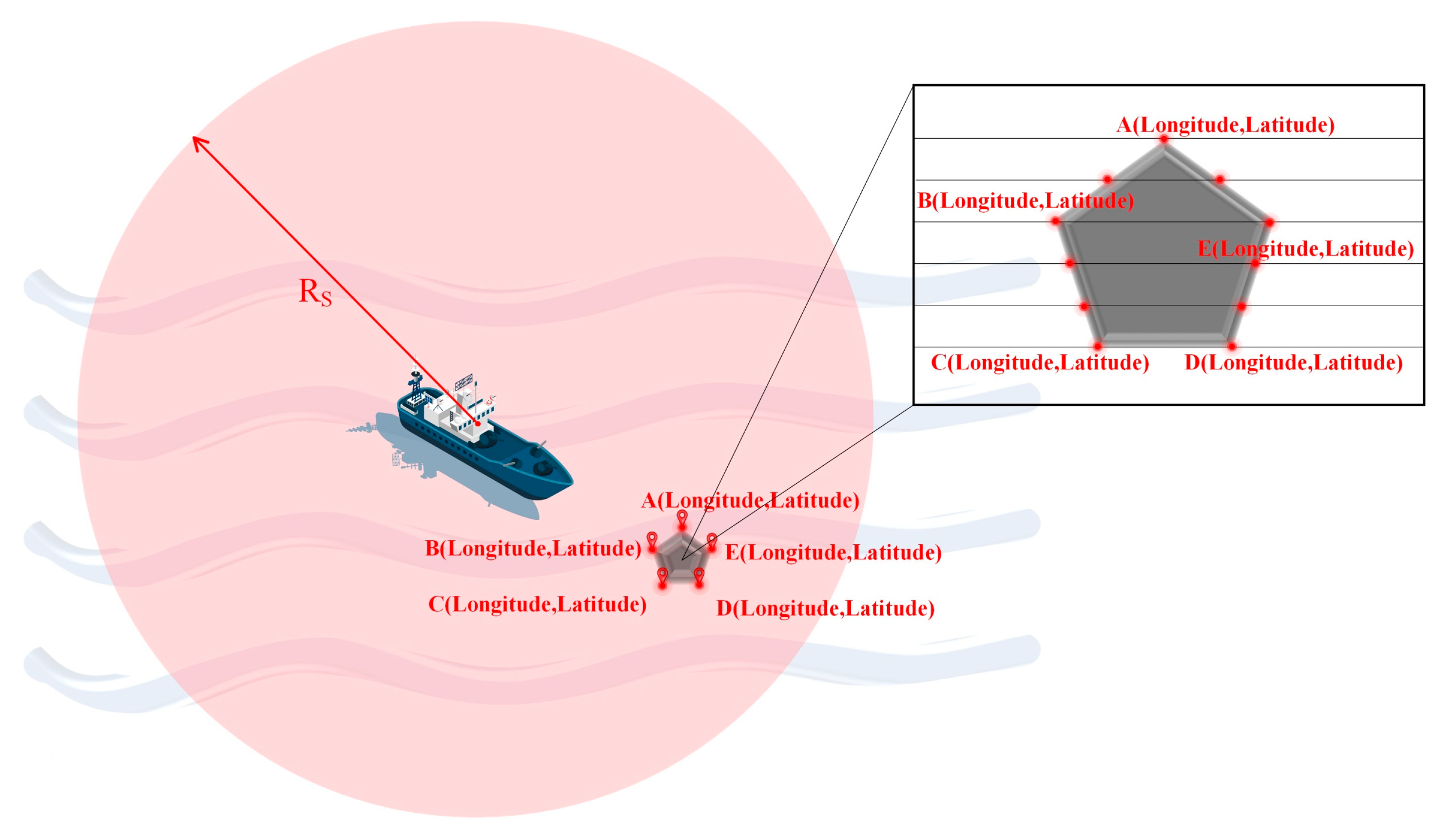
3.1. Patrol Information Graph

Assume a multi-USV system with N U nodes is performing a cooperative patrol mission within a rectangular task area A of size L M × L N .Given that the nodes are sailing on the water surface, the area A can be simplified into a two-dimensional plane, and the nodes are projected onto A for analysis. When constructing the patrol information graph, the first step is to rasterize the area A . The size of each grid L x × L y should be determined based on the detection range of the sensors carried by the nodes. To simplify the analysis, the area measurable by the sensor within a unit of time is approximated as a circular region with a detection radius of R s . Areas outside the detection radius cannot be surveyed for the required task information. After rasterizing area A , the task region g to be covered is represented by the center coordinates m , n of each grid:
g = m , n , m 1,2 , 3 , L M L x , n 1,2 , 3 , L N L y
The patrol information value obtained by a USV ( U S V i ) at time k is represented by λ i , g k . A downward-facing RGB-D camera (FoV 90° × 60°, resolution 1280 × 720) captures water surface features. The coverage state λ i , g k is determined by whether the grid g is within the camera’s frustum and satisfies texture recognition criteria. When λ i , g k = 1 , it indicates that the patrol information for region g has been acquired by U S V i at time k . When λ i , g k = 0 , it means that the patrol information for region g has not yet been acquired by U S V i at time k . Therefore, as shown in Figure 5, the patrol information acquired by U S V i at time k is represented as E i k :
E i k = λ i , g k g A
Due to the limitations of the sensor’s perception range, a single node can only acquire partial patrol information for the task area. However, by establishing an appropriate information exchange mechanism, a single node can obtain the patrol information of other nodes, thereby enabling it to gain a more comprehensive understanding of the task situation. Communication between nodes forms the foundation for establishing an information fusion mechanism. Similar to the node’s perception capability, the communication capability of a node is also constrained by both the device and the environment, which means that it can only communicate with other nodes within a specific range. Other nodes located within the communication radius R c of U S V i at time k are defined as U S V i ’s “neighbors”, denoted as N e i k :
Ν e i k = j | i , j μ i k μ j k R c i
μ i k and μ j k represent the positions of U S V i and U S V j , respectively, in the task area at time k . At time k , U S V i patrols and acquires E i k . It then sends E i k to other neighbors while simultaneously receiving the patrol information from them. U S V i merges and updates E i k with the patrol information obtained from other neighbors according to the following rules: U S V i updates the corresponding positions in E i k where it has not yet acquired patrol information, but other neighbors have. Specifically, U S V i updates the patrol information value at those positions from 0 to 1. If U S V i has already acquired the patrol information at a given position, no update is made for that position. The updated E i k is denoted as E ~ i k .

3.2. Cooperative Information Graph

As indicated by the previous description, the collaboration between USVs is a critical system characteristic of multi-USV systems, and it represents the greatest advantage of such systems over single USV in practical missions. In the cooperative patrolling task of multi-USV systems, to fully leverage the system’s cooperative features, the nodes in the system, when making task decisions, need to not only maximize their own operational efficiency but also consider the operational information of other nodes (referred to as teammates) within the system as a key reference for decision-making. This approach ensures that the generated algorithm can maximize the overall operational effectiveness of the system.
To address this, a cooperative information graph is introduced in the patrol situation model. This information graph is constructed based on the Long Short-Term Memory (LSTM) artificial neural network model. With the aid of this model, the position of other nodes at the next time step can be predicted based on the information acquired from these nodes, thereby generating the corresponding cooperative information graph. By utilizing the cooperative information graph, nodes can fully consider the operational status of their teammates at the next time step when generating control commands. This approach ensures a rational distribution of tasks among the nodes in the system, avoids conflicts, fosters collaboration between them, and maximizes the system’s task capability. Additionally, it prevents redundant patrolling of the same area by multiple nodes during the mission, thereby improving the operational efficiency of the system.
In the node position dynamic prediction model, the input consists of the dynamic motion information of teammates, which exhibits a clear sequential characteristic. As a result, statistical prediction models are not suitable for this type of input. The LSTM model, however, addresses this issue by incorporating gate structures, including the input gate, forget gate, and output gate, to regulate the flow of information. This mechanism determines which information should be retained and which should be discarded, effectively mitigating the limitations of traditional RNN networks. In the teammate state prediction model, the historical data of teammates’ states are used as input data. The input sequence data is represented as: X = X 1 , X 2 , , X T , where X T = x t 1 , x t 2 , , x t L X , and L represents the time step, meaning that the teammate’s next state is predicted based on the teammate’s historical state over the past L time steps.The hidden state of the LSTM memory unit is denoted as H = h 1 , h 2 , , h T , and the output time series is represented as Y ^ = y ^ 1 , y ^ 2 , , y ^ T , where y ^ t = h T serves as the predicted value of the teammate’s next state. The weight of the input weighting layer is defined as:
W = w 1 , w 2 , , w L
After importance weighting through the input weighting layer, the input data to the LSTM module can be represented by the Equations (4) and (5) as shown below:
X ~ = x ~ 1 , x ~ 2 , , x ~ T
X t ~ = w 1 x t 1 , w 2 x t 2 , , w L x t L
The nonlinear mapping function of the memory unit in the LSTM is shown as follows:
f t = σ W f h t 1 , X ~ t + b f
i t = σ W i h t 1 , X ~ t + b i
c t = f t c t 1 + i t tanh W c h t 1 , X ~ t + b c
o t = σ W o h t 1 , X ~ t + b o
where W f ,   W i ,   W c ,   W o are the weight matrices for the forget gate, b f ,   b i ,   b c ,   b o are the corresponding bias vectors, σ is the sigmoid activation function, f t is the forget gate state, i t is the input gate state, c t is the cell state, o t is the output gate state, and h t represents the hidden layer output. Based on the node position prediction model, U S V i is capable of obtaining the predicted position of neighboring nodes within its communication radius at time k for the next time step. The predicted position information of neighboring nodes at the next time step is added to the grid map of size A to form the cooperative information graph C i k at time k for U S V i , as shown in Equation (11):
C i k = v i , g k g A
When v i , g k = 1 , it indicates that the region g will be occupied by a teammate at the future time step. When v i , g k = 0 , it indicates that the region g will not be occupied by a teammate at the future time step.

3.3. Obstacle Information Map

In real-world task scenarios, nodes are affected by obstacles during their navigation process. These obstacles can be categorized into two types: the first type is dynamic obstacles, such as other ships sailing on the water surface and other navigation nodes in the system; the second type is static obstacles, such as islands, reefs, large buoys, and so on.
It is assumed that during its navigation, U S V i ’s onboard sensors are capable of extracting and returning obstacle information within a detection radius of R s . For static obstacles, which are typically large in volume, it is necessary to process the static obstacle information obtained by the sensors to ensure the safety of the node’s navigation. Each USV integrates a 360° LiDAR (detection radius R s = 1 00 m, angular resolution 0.1°) and a side-scan sonar (range 50 m, frequency 500 kHz) for obstacle detection.
The specific processing method is as follows: As shown in Figure 6, if the polygon ABCDE represents an obstacle detected by U S V i , the returned obstacle information will consist of the latitude and longitude coordinates of the vertices of the polygon ABCDE.
After obtaining the latitude and longitude information of the obstacle vertices, the obstacle data provided by the sensor is extracted into binary information in the raster map using the Scan-Line Fill method [32]. As shown in Figure 6, the polygon ABCDE represents the obstacle detected by U S V i in region R s at time k . At this point, the Scan-Line Fill method generates multiple equidistant scan lines, which intersect with the edges of the obstacle at several points. For a closed-shaped obstacle, the intersection points between the equidistant scan lines and the obstacle edges always occur in pairs. From left to right, these intersections alternately enter and exit the obstacle, meaning the region between two intersection points corresponds to the area occupied by the obstacle. The corresponding raster in this region is marked as the obstacle grid. Based on the positional information of these 12 intersection points, the corresponding obstacle information can be formed in the raster map (with the raster information at the intersection points set to 1). For dynamic obstacles, which have a smaller volume, they are treated as nodes for analysis and processing during the obstacle avoidance process. Both dynamic and static obstacles are added to the grid map of size 2 R s × 2 R s , resulting in the obstacle information map O b i k for U S V i :
O b i k = o i , g k g A
When o i , g k = 1 , it indicates that a dynamic obstacle exists within U S V i ’s node safe navigation distance threshold R a c o l l i s i o n at time k . When o i , g k = 2 , it indicates that a static obstacle exists within U S V i ’s obstacle safe navigation distance threshold R o c o l l i s i o n at time k . When o i , g k = 0 , it indicates that no obstacle exists within both R a c o l l i s i o n and R o c o l l i s i o n at time k for U S V i .

4. Proposed Strategy

The complex maritime environment and specific mission context place higher demands on USVs, requiring faster response times to quickly generate corresponding control commands after obtaining situational information, thereby enhancing the system’s real-time control performance. Based on this, this paper proposes a cooperative patrol control strategy based on hybrid embedded task state information, using an improved OODA model control architecture. The strategy combines time-triggered and event-triggered task state information to achieve a more efficient and cooperative patrol control method. By adopting the improved OODA model control architecture, the traditional non-end-to-end decision-making process is transformed into an end-to-end decision-making process. Through reward reshaping and the rational design and adjustment of reward signals, the strategy significantly improves the learning efficiency of the cluster nodes, making the trained strategy particularly suitable for the highly dynamic and real-time response requirements of multi-USV cooperative patrol missions. This section will provide a detailed analysis of the strategy.

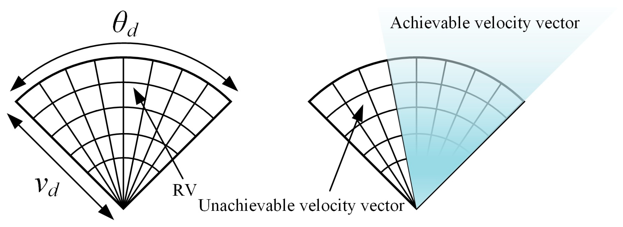
4.1. Action State Output of Unmanned Surface Vehicles Based on the Dynamic Window

For an agent, the policy refers to the mapping relationship from state to action. Therefore, the node needs to have the capability to provide accurate and comprehensive mission situational information. Based on the previously constructed mission state information model, the patrol information graph E ~ i k collaboration information graph C i k , and obstacle information graph O b i k obtained by U S V i at time k are considered as the mission situational information, or state value S i k :
S i k = E ~ i k , C i k , O b i k
The motion space of the agent is closely related to the agent’s dynamics and kinematics characteristics. The action a i k of U S V i at time k is expressed as follows:
a i k = τ i , u k , τ i , r k
In Equations (13) and (14),   S i k serves as the input to policy network, a i k represents the control output of U S V i at time k , where τ i , u k and τ i , r k are two continuous variables representing the forward thrust and yaw moment of U S V i at time k , respectively. Based on the kinematic and dynamic model of the USV established, the motion state information of U S V i at time k can be calculated after applying the corresponding a i k . However, due to the limitations of the USV’s dynamic performance, there are certain velocity vectors that the node cannot achieve in the current motion state, regardless of the control input. Therefore, considering the dynamic performance of the USV, the dynamic window algorithm is used to derive the achievable movement speed of the USV within a given time window, referred to as the velocity window v w i n d o w :
v w i n d o w = v | v v c v ˙ Δ k , v c + v ˙ Δ k
and the achievable angular velocity, referred to as the angular velocity window ω d :
ω w i n d o w = ω | ω ω c ω ˙ Δ k , ω c + ω ˙ Δ k
In Equation (15), v c is the current movement speed of USV. v ˙ is the acceleration of the USV, and Δ k is the duration of the control input.
In Equation (16), ω c is the current angular velocity of the USV, and ω ˙ is the angular acceleration of the USV. Based on Equation (16), the achievable heading angle range of the USV within time Δ k can be calculated:
θ w i n d o w = θ | θ θ h + ω c Δ k 1 2 ω ˙ Δ k 2 , θ h + ω c Δ k + 1 2 ω ˙ Δ k 2
θ h is the current heading of USV. Using Equations (14) and (16), the values of v w i n d o w and θ w i n d o w can be determined. However, the elements in the sets of v w i n d o w and θ w i n d o w are continuous, which makes engineering calculations difficult. Therefore, as shown in Figure 7, v w i n d o w is discretized into M speeds, and θ w i n d o w is discretized into N heading directions. Each discrete speed v d i s c r e t e and heading θ d i s c r e t e form a set of velocity vectors v d i s c r e t e , θ d i s c r e t e , and these velocity vectors are referred to as the achievable velocities (RV).
When U S V i takes the corresponding action a i k at time k , the velocity vector corresponding to the current node’s motion state is calculated. Then, the closest velocity vector from the RV (reachable velocities) is selected as the velocity vector of U S V i after adopting a i k . Based on this chosen velocity vector, the dynamics information after U S V i adopts a i k is computed.

4.2. Reward Function Design

The appropriate reward values not only enable nodes to learn the optimal task strategy based on task situation information, but also effectively prevent nodes from encountering issues such as non-convergence or getting stuck in local optima during the learning process. Before designing the reward values for the nodes, it is essential to first clarify the objectives of the task being executed by the system. The objectives of a multi-unmanned vessel system performing a cooperative patrol task are as follows:
  • The system should be able to acquire patrol information of the entire task area.
  • Under the condition of acquiring task data for the entire task area, patrol efficiency should be maximized and task costs minimized.
  • Ensure the safety of all nodes during navigation, avoiding collisions between nodes and obstacles.
Based on the task environment settings mentioned above, in traditional strategy training, nodes can only receive the final reward r c o v e r after completing full coverage of the task area, and they receive an efficiency reward r e f f i e n c y according to the completion status. However, these rewards are only given at the end of the task, and the reward structure often exhibits high sparsity, meaning that clear feedback is only provided when the task is fully completed. This delayed feedback mechanism has a significant negative impact on the learning process, leading to the problem of reward sparsity. The core of this issue lies in the fact that during the learning process, agents struggle to establish clear causal relationships and cannot promptly associate specific actions or states with the eventual success of the task. The challenges posed by sparse rewards are multifaceted.
Firstly, it severely hampers the agent’s effective exploration of the environment. In the absence of timely feedback, the agent struggles to determine which actions are beneficial and which are ineffective or harmful. This forces the agent to engage in extensive random exploration, hoping to discover valuable state-action sequences through chance attempts. However, this approach is not only time-consuming but also computationally expensive, especially in tasks with large state spaces or complex action spaces, such as a water patrol task.
Secondly, the issue of sparse rewards can lead to the learning process getting trapped in local optima. Due to the lack of intermediate feedback, the agent may prematurely converge on strategies that seem effective but are not globally optimal. In this case, the agent struggles to break free from its current behavior patterns to explore potentially better solutions, as it lacks sufficient motivation and guidance to try new, higher-risk but higher-reward behaviors.
To address these issues, this paper combines reward reshaping techniques. The core idea of this method is to cleverly design and introduce a series of intermediate reward signals on top of the original sparse rewards. These additional rewards serve as immediate feedback during the task, providing more granular and information-rich guidance for the learning process. Reward reshaping techniques offer more dense and informative feedback by incorporating extra intermediate rewards based on the original reward signals. This approach can significantly accelerate the learning process, helping the agent discover valuable behavioral patterns more quickly. Through the carefully designed reward function, we can integrate domain knowledge or prior information into the reward structure, guiding the agent to explore in the desired direction. This not only improves learning efficiency but also enhances the quality of the final policy.
By combining reward reshaping, we can break down complex long-term goals into a series of more easily learnable short-term sub-goals. This decomposition accelerates the learning process and helps the agent quickly identify and reinforce valuable behaviors. Therefore, by introducing additional reward functions to “shape” the agent’s learning path, the agent receives more feedback during exploration, thus accelerating the learning process. This paper reconstructs the reward structure and assigns corresponding rewards based on the state value obtained by the node. The rewards are divided into patrol reward, cooperative reward, obstacle avoidance reward, and efficiency reward.

4.2.1. Patrol Reward

This section of the reward represents the dense immediate rewards introduced in the reward mapping. The traditional reward r c o v e r is transformed into a coverage reward r c o v e r k that can be obtained at each time step. The strategy assigns patrol rewards to the nodes based on their patrol status in the task area. The reward value is mainly determined by the node’s information collection in the task area. The patrol reward consists of two main components: coverage reward and completion reward. The coverage reward obtained by node U S V i at time step k is represented as r i c o v e r k :
r i c o v e r k = g E ~ i k λ i , g k   i f   λ i , g k 1 = 0 λ i , g k = 1  
The equation indicates that the algorithm will reward the node for acquiring new patrol information in the task area. In other words, when the node’s actions lead to the system obtaining more patrol information, the node will receive the corresponding reward.
When the entire task area is covered, U S V i will be given a completion reward r i f i n i s h k :
r i f i n i s h k = g E ~ i k λ i , g k
Finally, the patrol reward for U S V i at time step k is given by the Equation (20) as follows:
r i e x p l o r a t i o n k = β c o v e r r i c o v e r k + β f i n i s h r i f i n i s h k
where,   β c o v e r is the weighting coefficient for the coverage reward, prioritizing exploration of new areas. A higher value encourages nodes to focus on uncovering unexplored regions.   β f i n i s h is the weighting coefficient for the completion reward, emphasizing full coverage of the task areas. A higher value incentivizes nodes to collectively achieve complete surveillance.

4.2.2. Cooperative Reward

This section of the reward represents the intensive, immediate rewards introduced in the reward mapping. In order to maximize the patrolling capability of each node within the multi-unmanned vehicle system, and to avoid redundant patrolling of the same location by nodes in the system (before the entire task area is covered, redundant patrolling will lead to a waste of system resources and significantly increase the risk of collisions between nodes, which has a significant negative impact on the operational efficiency of the system), a cooperative reward r i c o o p e r a t i o n k is established for each node. This reward is determined based on the cooperative information map C i k obtained by U S V i :
After taking the corresponding action a i k at time k , U S V i obtains the cooperative information map C i k + 1 at time k + 1 . First, the task areas within C i k + 1 that have a value of 1 are identified, and the distance D i s t i j k + 1 between these areas and U S V i at time k + 1 is calculated. These distances are then organized into the corresponding distance set:
D i s t c o o p e r a t i o n k + 1 = D i s t i 1 k + 1 , D i s t i 2 k + 1 , , D i s t i j k + 1
The calculation of D i s t i j ( k + 1 ) is shown in Equation (22):
D i s t i j k + 1 = x i k + 1 m 2 + y i k + 1 n 2
where, x i k + 1 , y i k + 1 represents the x and y coordinates of U S V i ’s position at time k + 1 , and m , n refers to the coordinates of the task areas in C i k + 1 that satisfy v i , g k = 1 .
r i c o o p e r a t i o n k = Ν e i k , i f   D i s t i j D i s t c o o p e r a t i o n ( k + 1 ) > D i s t g a t e 1 Ν e i k 1 / N U e T i ( k ) , e l s e
where, D i s t g a t e represents the distance determination threshold, and T i k denotes the total operation time of U S V i up to time k .

4.2.3. Obstacle Avoidance Reward

This section of the reward is a dense immediate reward introduced in the reward mapping. In the cooperative patrolling task of a multi-unmanned boat system, obstacle avoidance at the nodes is a critical issue that must be considered. Only by equipping the nodes with effective obstacle avoidance capabilities can the system prevent collisions between nodes and between nodes and obstacles in the task areas, thereby avoiding damage to the nodes and improving the system’s operational efficiency. Therefore, U S V i will receive the corresponding obstacle avoidance reward r i a v o i d   c o l l i s i o n k at time k , ensuring that the task strategy generated after node training has the necessary obstacle avoidance capability. r i a v o i d   c o l l i s i o n k consists of two parts: the node’s obstacle avoidance reward r i n o d e   c o l l i s i o n k and the obstacle’s avoidance reward r i o b s t a c l e   c o l l i s i o n k .
r i n o d e   c o l l i s i o n k is designed using the obstacle information map O b i k and based on the Artificial Potential Field (APF) method. Using APF, the node calculates the interaction danger force F i j k + 1 between each pair of nodes in the system and their corresponding force vectors F i k + 1 . Then, based on F i k + 1 , the corresponding action a i k taken by U S V i at time k is determined. The calculation process for F i j k + 1 is as follows:
After U S V i takes the corresponding action a i k at time k + 1 , it obtains the obstacle information map O b i k + 1 for time k + 1 . First, the distance D i s t i j k + 1 between the regions with a value of 1 in O b i k + 1 and U S V i at time k + 1 is calculated, and the corresponding distance set is formed as follows:
D i s t a c o l l i s i o n ( k + 1 ) = D i s t i 1 ( k + 1 ) , D i s t i 2 ( k + 1 ) , , D i s t i j ( k + 1 )
If there are no regions with a value of 1 in O b i k + 1 then D i s t a c o l l i s i o n ( k + 1 ) = . The calculation method for D i s t i j ( k + 1 ) is shown in Equation (25):
D i s t i j k + 1 = x i k + 1 m 2 + y i k + 1 n 2
where, x i k + 1 , y i k + 1 represents the x and y coordinates of U S V i at time k + 1 , and m , n refers to the coordinates of the region in O b i k + 1 that satisfy Equation (26):
o i , g k + 1 = 1 o i , g k = 1
Therefore, the F i j k + 1 for U S V j is calculated using Equation (27):
F i j k + 1 = δ e α D i s t i j k + 1 , D i s t i j k + 1 D i s t a c o l l i s i o n ( k + 1 ) < D i s t s a f e t y 0 ,   D i s t i j k + 1 D i s t a c o l l i s i o n ( k + 1 ) > D i s t s a f e t y D i s t a c o l l i s i o n ( k + 1 ) =
where, δ and α are adjustable parameters. In order to provide sufficient obstacle avoidance reaction time for nodes in relation to other nodes in the region and ensure the safety of the node’s navigation, a “dilation” process is applied. The dilated node becomes a circular region with a radius r U S V . During training, “pseudo” collisions can be penalized to provide the node with more obstacle avoidance reaction time, thereby enhancing the obstacle avoidance capability between nodes. Based on the above reasons, the safety navigation distance threshold between nodes is:
D i s t s a f e t y = 2 r U S V
F i k + 1 is the resultant force vector generated by all the nodes within O b i k + 1 that meet the conditions, expressed as:
F i k + 1 = i j F i j k + 1
Finally, based on F i k + 1 , r i n o d e   c o l l i s i o n k is calculated using Equation (30):
r i n o d e   c o l l i s i o n k = e δ d a n g e r o u s F i ( k + 1 ) , F i ( k + 1 ) 0 , N a i ( k ) , F i ( k + 1 ) = 0 .
where, δ d a n g e r o u s is the danger force cost parameter, where δ d a n g e r o u s = 0.6 . N a i k is the set of regions within O b i k where the value is 1.
r i o b s t a c l e   c o l l i s i o n k is similarly designed using the information from the obstacle map O b i k . First, the distance O b i k + 1 between the task area with a value of 2 in O b i k + 1 and U S V i is calculated, forming the corresponding distance set:
D i s t o c o l l i s i o n ( k + 1 ) = D i s t i 1 ( k + 1 ) , D i s t i 2 ( k + 1 ) , , D i s t i j ( k + 1 )
If there are no regions with a value of 2 in O b i k + 1 , then D i s t o c o l l i s i o n ( k + 1 ) = . The calculation of D i s t i j ( k + 1 ) is shown in Equation (32):
D i s t i j k + 1 = x i k + 1 m 2 + y i k + 1 n 2
where, x i k + 1 , y i k + 1 represents the coordinates of U S V i at time k + 1 . m , n are the coordinates of the task region in O b i k + 1 where o i , g k + 1 = 2 o i , g k = 2 . The calculation process for r i a r e a   c o l l i s i o n k is shown in Equation (33):
r i o b s t a c l e   c o l l i s i o n k = r s i z e min   D i s t i j k + 1   i f   D i s t i j k + 1 D i s t o c o l l i s i o n k + 1 < r s i z e N o i k ,   D i s t i j k + 1 D i s t o c o l l i s i o n k + 1 > r s i z e D i s t o c o l l i s i o n k + 1 =
N o i k is the set of regions in O b i k where the value is 2. Similarly, in order to provide sufficient time for the nodes to react to the obstacles in the region and improve the obstacle avoidance effectiveness, the detected static obstacles are “inflated”, which means the obstacle region’s range is expanded. The inflated obstacle becomes a circular region with a radius r a r e a . Therefore, when the following condition is met:
D i s t i j ( k + 1 ) < r s i z e
The node is considered to have “collided” with the obstacle region when the condition is met. At this point, the node will receive a corresponding negative reward, where:
r s i z e = r a r e a + r U S V
The final r i a v o i d   c o l l i s i o n k is shown in Equation (36):
r i a v o i d   c o l l i s i o n ( k ) = β n o d e   c o l l i s i o n r i n o d e   e   c o l l i s i o n ( k ) + β a r e a   c o l l i s i o n r i a r e a   c o l l i s i o n ( k )

4.2.4. Efficiency Reward

This section of the reward is the sparse terminal reward introduced in the reward mapping. As previously mentioned, one of the main objectives of the task strategy generated by the node is to maximize work efficiency while ensuring full coverage of the task area, thereby reducing the task cost. To achieve this, an appropriate efficiency reward value r i e f f i c i e n c y k is designed for the node.
r i e f f i c i e n c y k is used to evaluate the efficiency of the task strategy generated by the node from a time perspective. It is known that, under the same task conditions, the time required for the node to complete a patrol from the start to the stop (i.e., when the system finishes one episode) is called the patrol time k i , e p i s o d e for U S V i . The shorter the k i , e p i s o d e in the system, the higher the efficiency of the patrol strategy used by U S V i . Therefore, the efficiency reward value received during U S V i ’s learning process will be higher. Conversely, if the patrol strategy used by U S V i is less efficient, the efficiency reward value received by U S V i will be lower. The efficiency reward r i e f f i c i e n c y k obtained by U S V i at time k is calculated by Equation (37):
r i e f f i c i e n c y k = 0 , k i , e p i s o d e > c 1 T k B e n c h m a r k r B e n c h m a r k 2 1 + c o s π T c 2 T k B e n c h m a r k c 1 T k B e n c h m a r k c 2 T k B e n c h m a r k r m a x , k i , e p i s o d e c 1 T k B e n c h m a r k , c 2 T k B e n c h m a r k < k i , e p i s o d e c 1 T k B e n c h m a r k
In Equation (37), r B e n c h m a r k is the baseline efficiency reward for the node when executing the task, and c 1 T and c 2 T are correction factors. k B e n c h m a r k is the baseline time for the node to complete the task, which is calculated as follows:
k B e n c h m a r k = m i n L y 1 L M L x L y v m a x + L x 1 L N L x v m a x , L x 1 L N L y L x v m a x + L y 1 L M L y v m a x
In Equation (38), v m a x represents the maximum speed of the node under ideal conditions. Therefore, the reward value r i k obtained by U S V i at time k is given by Equation (39) as follows:
r i k = β T r = β exploration β c o o p e r a t i o n β a v o i d   c o l l i s i o n β e f f i c i e n c y T r i exploration k r i c o o p e r a t i o n k r i a v o i d   c o l l i s i o n k r i e f f i c i e n c y k
From Equation (39), it can be seen that a constant vector is used to weight various types of reward values. This is because the relative magnitude of the reward values generated by different types of reward terms also has a significant impact on the process of the node’s learning task strategy. Therefore, in order to ensure that different reward terms have distinct effects during the training process, ultimately enabling the system to learn a task strategy that meets the task requirements, a constant vector β is used to weight various types of reward values.
During the execution of the patrol task, the primary concern is ensuring the navigational safety of the task nodes, so r i a v o i d   c o l l i s i o n k has the largest weight in r i k . Next, to achieve good operational efficiency, r i e f f i c i e n c y k also carries a relatively large weight in r i k .
In the early stages of the task, the system’s nodes need to patrol the task area in a more dispersed manner to fully utilize each node’s patrol capabilities. As a result, r i c o o p e r a t i o n k carries more weight than r i e x p l o r a t i o n k during this phase. In the later stages of the task, the system needs to maximize the patrol rate in the task area, concentrating the system nodes in the unpatrolled regions, so the weight of r i e x p l o r a t i o n k becomes larger in this phase. So:
β exploration = 0.5 + 1 e T i ( k )
β c o o p e r a t i o n = 0.5 1 e T i ( k )
The weight decays with mission time T i ( k ) . Early in the mission ( T i ( k ) 0 ),   β c o v e r 1.5 prioritizes exploration. Later ( T i ( k ) ), β c o v e r 0.5 shifts focus to collaborative convergence. This mechanism enables real-time strategy adaptation based on mission progress.

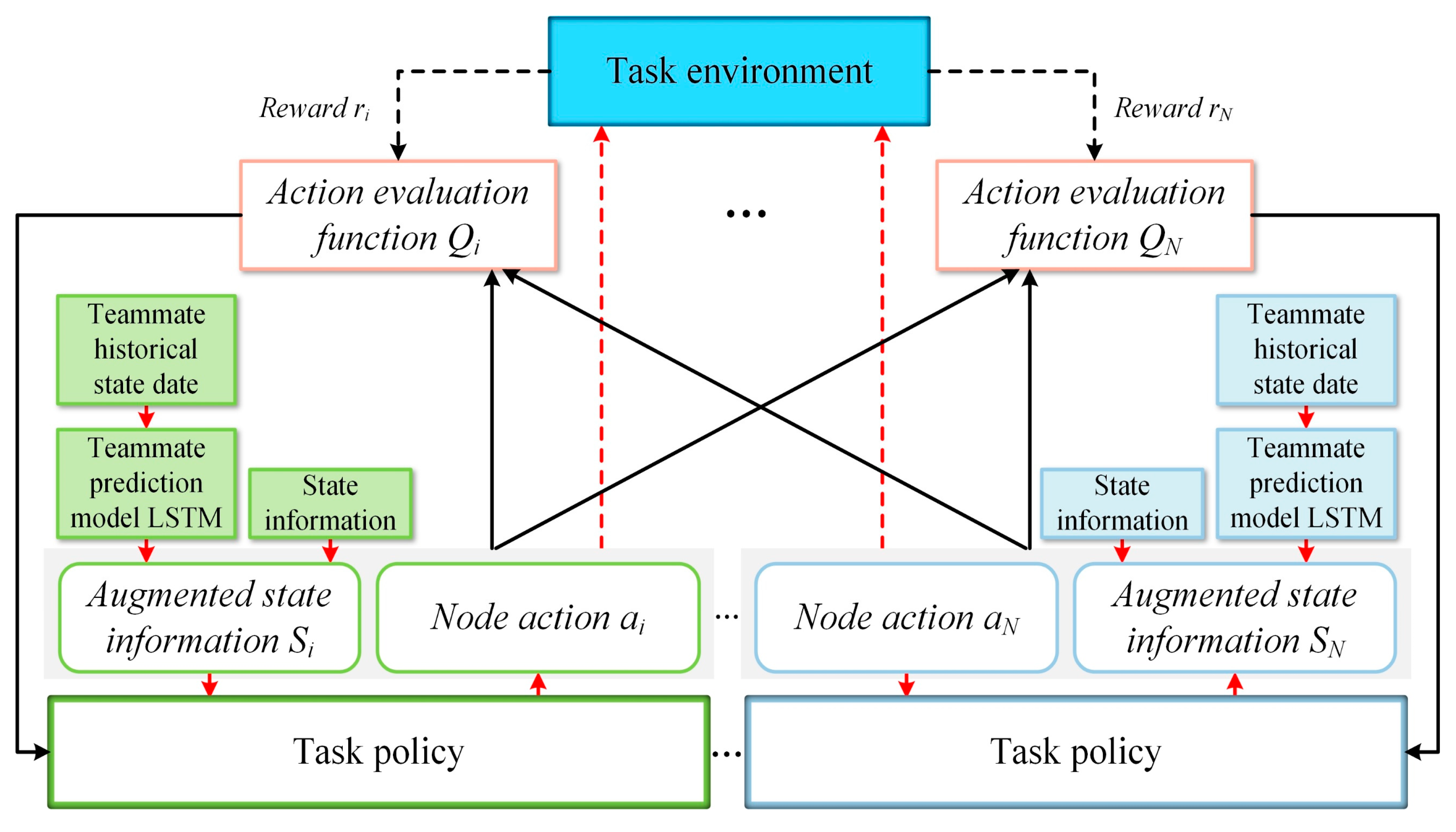
5. Strategy Training

5.1. Training Process

The Training Framework for Multi USV(TFMUSV) is shown in Figure 8. The specific training process is as follows:
On U S V i , the interception strategy μ i and action evaluation function Q i run independently. U S V i predicts the next state of its teammate based on historical state data, using the teammate state prediction model, generating augmented state information s i . Following strategy μ i , it selects action a i and receives the environmental feedback reward signal r i . The joint state information and joint actions of the USV swarm are input into the action evaluation function in the training framework. After calculating the gradient information, the policy network P and action evaluation network Q in the training framework are updated. The objective function corresponding to the action evaluation network Q is:
L θ = E S i k , a i k , ot S i k _ a i k , r i k , S i k + 1 D
[ Q ( S i k , a i k , o t S i k _ a i k θ ) r i k + Q ( S i k + 1 , a i k + 1 , ot S i k + 1 _ a i k + 1 θ ) 2 ]
In Equation (42), ot S i k _ a i k represents the states and actions of other nodes in the multi-agent system. For the state and action at the next time step ot S i k + 1 _ a i k + 1 , the state ot S i k + 1 comes from the replay buffer, and the corresponding action ot a i k + 1 is obtained through the delayed policy network. The gradient update is as shown in Equation (43). For the policy network, the corresponding objective function is:
J ( μ ) = E S i k , ot S i k _ a i k D [ Q ( S i k , P S i k , a i k μ , ot S i k _ a i k θ ) ]
The gradient calculation method for Equation (43) is shown in Equation (44):
𝛻 μ J μ = E S i k , ot S i k _ a i k D [ 𝛻 θ P S i k , a i k μ   𝛻 a Q ( S i k , a i k , ot S i k _ a i k θ ) a i k = P S i k μ ]
Then, the parameters μ in the policy network P are updated through gradient ascent in Equation (45):
μ = μ + η μ J ( μ )
The pseudocode for the training of the multi-USV cooperative training framework proposed in this paper is shown in Algorithm 1, and the multi-USV cooperative training framework is shown in Figure 8.
Algorithm 1 Multi-USV cooperative Patrol Control algorithm
Require: Multi-agent N U , Policy network μ i , Q Network parameters θ i , i = 1   t o   N U
Replay buffer D
1: Assign target network parameters μ μ , θ θ
2: for i = 1   t o   N U do
3:   μ i μ i , θ i θ i
4: end for
5: while not stop do
6:   for k = 1 : m a x _ e p i s o d e _ l e n g t h do
7:      Obtain the current environment state S i k , and obtain a i k based on   P i .
8:      a i k = P S i k μ + ε , ε N   ( N is noise)
9:      end for
10:    Execute action a 1 k , a 2 k , a M k to obtain reward r 1 k , r 2 k , r M k and add new state values s 1 k + 1 , s 2 k + 1 , s M k + 1 , and add them to D
11:    if s 1 k + 1 , s 2 k + 1 , s M k + 1 is the terminal state, then
12:      Reset the environment
13:     break
14:    end if
15:  end for
16:  Randomly sample b from D , and add it to B .
17:  for i = 1   t o   N U do
18:    Calculate the Q-value, y i = r i k + γ Q ( S i k + 1 , a i k + 1 , o t h e r S i k + 1 θ )
19:   Update the Q-value network parameters
20:     θ θ 𝛻 θ 1 B S i k , a i k , o t h e r S i k _ a i k B Q S i k , a i k , o t h e r S i k a i k θ i y i 2
21:   Update the policy network parameters
22:   μ μ 𝛻 μ 1 B S i k , o t h e r S i k _ a i k B Q ( S i k , P S i k μ i , o t h e r S i k _ a i k θ i )
23: for i = 1   t o   N U do
24:    Update the target network parameters:
25:     μ i ρ μ i + 1 ρ μ i
26:     θ i ρ θ i + 1 ρ θ i
27:    end for
28: end while

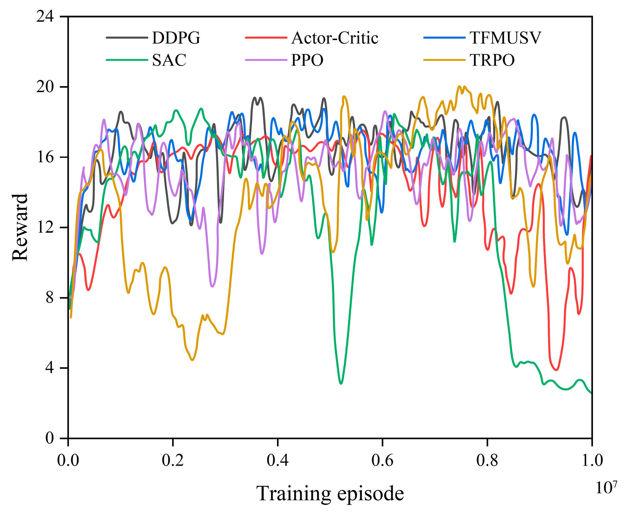
5.2. Training Result
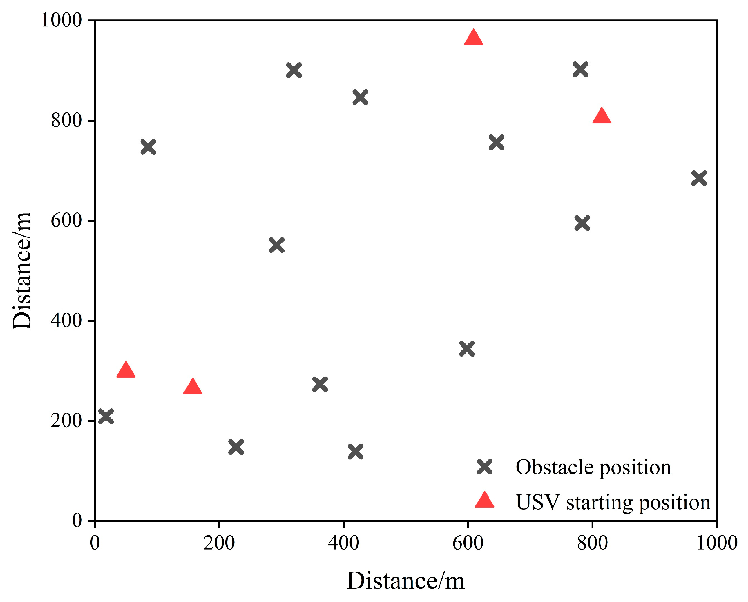
A simulation training environment based on Python 3.12 is built using Google’s TensorFlow 2.15. All training and simulations were conducted on a server equipped with an Intel Xeon Gold 6248R CPU, 256GB RAM, (manufactured by Intel Corporation, headquartered in Santa Clara, CA, USA) and two NVIDIA RTX A6000 GPUs (manufactured by NVIDIA Corporation, headquartered in Santa Clara, CA, USA). The TensorFlow framework leveraged GPU acceleration for parallelized experience replay and batch gradient computation. This training environment is designed to simulate various task scenarios in a multi-unmanned vehicle system cooperative patrol mission. As shown in Figure 9, a training task area of 1000 × 1000   m 2 is set in the environment. N obstacles are randomly placed within the task area, represented by the rectangular blocks in Figure 9. The performance parameters and dynamics models of the unmanned vehicles in the simulation environment are set and modeled based on the unmanned vehicles used in actual vessel tests. The hyperparameters required during the training process are provided in Table 1.
Different types of training frameworks were also used to train the system during the training process. The training results of various algorithms are shown in Figure 10. The changes in the reward values obtained by the nodes throughout the training period are presented for the training frameworks of DDPG, Actor-Critic, SAC, PPO, and TRPO. As shown in the results of Figure 10, when the system used the Actor-Critic, SAC, and TRPO frameworks during training, the reward values obtained by the system could not remain in a stable upward state, and the reward fluctuations were always large, failing to converge throughout the training. In particular, with the SAC algorithm, the reward values obtained by the system even decreased during the later stages of training. This indicates that these three training frameworks are not suitable for training the system, as they cannot help the system learn an effective task strategy.
From the analysis of Figure 10, it can be observed that the three training frameworks (DDPG, TFMUSV, and PPO) can help the system achieve higher rewards during the training process compared to the other three frameworks. However, in the later stages of training, although the reward values tend to converge, the fluctuations remain large. Based on this, using these three training frameworks, and adjusting the weight coefficients of different reward values in the reward function according to the weight coefficient combinations provided in Table 2, the system is retrained. Figure 11 shows the training results when using the F combination. From Figure 11, it can be seen that, under the DDPG, TFMUSV, and PPO training frameworks, the trends of the node reward values are similar, but further analysis reveals that TFMUSV results in significantly higher initial rewards for the nodes compared to the other two frameworks. Additionally, in the later stages of training, DDPG and PPO lead to reward values that are clearly lower than those obtained with TFMUSV, and the reward value fluctuations in the later stages of training are also significantly smaller in TFMUSV compared to DDPG and PPO. The training results indicate that, compared to the other two training frameworks, TFMUSV enables the system to learn more effective task strategies, thereby allowing the system to achieve higher rewards during task execution.

6. Simulation Test

6.1. Test Evaluation Parameters

To verify whether the algorithm proposed in this paper can help the multi-unmanned vessel system efficiently and accurately complete the patrolling task, simulation testing was conducted on the trained system within the multi-unmanned vessel cooperative patrolling task simulation environment constructed in the earlier stages. During the testing process, several control algorithms currently applied in multi-agent cooperative patrolling tasks were used as comparisons to evaluate the performance of the algorithm proposed in this paper.
Before conducting the test, the performance parameters for evaluating the algorithm were first set. The performance parameters consist of several parts, namely patrol time T t o t a l , coverage R c o v e r , total navigation distance D t o t a l , CRBAA (Collision Rate Between Agent and Agent), and CRBAO (Collision Rate Between Agent and Obstacle). The calculation methods for each experimental parameter are shown in Equation (46):
T t o t a l = i = 1 N e p i s o d e T i e p i s o d e N e p i s o d e , i = 1,2 , , N e p i s o d e D t o t a l = i = 1 N e p i s o d e D i t o t a l N e p i s o d e , i = 1,2 , , N e p i s o d e R c o v e r = i = 1 N e p i s o d e S i c o v e r S A N e p i s o d e , i = 1,2 , , N e p i s o d e C R B A A = i = 1 N e p i s o d e N i c o l l i s i o n a g e n t s N i s t e p , i = 1,2 , , N e p i s o d e C R B A A = i = 1 N e p i s o d e N i c o l l i s i o n o b s t a c l e s N i s t e p , i = 1,2 , , N e p i s o d e
N e p i s o d e represents the total number of episodes. T i e p i s o d e represents the time required for the system to complete a certain episode. When T i e p i s o d e 3 T B e n c h m a r k , the episode will be terminated. D i t o t a l represents the total navigation distance of the system nodes during a certain episode. S i c o v e r represents the area covered by the system in the task region during a certain episode, and S A represents the actual area of the task region. N i c o l l i s i o n a g e n t s represents the number of collisions between nodes during a certain episode, and N i s t e p represents the total number of actions taken by the system nodes during that episode. N i c o l l i s i o n o b s t a c l e s represents the number of collisions between nodes and obstacles during a certain episode. Additionally, to simulate the patrolling information obtained during the task, different locations in the task area have different depths. When the node sensor covers the corresponding task area, the node will obtain the corresponding water depth data for that area, and the higher the completion of the task, the more complete the system’s water depth data for the task area will be.
In the comparison tests, the chosen algorithms were the anti-flocking-based cooperative patrolling control algorithm (referred to as the anti-flocking algorithm) and the partitioned scanning patrolling control algorithm (referred to as the partitioned scanning patrolling algorithm). Different testing scenarios were set based on different system scales during the test, as follows: Scenario 1: N U = 3 , Scenario 2: N U = 4 , Scenario 3: N U = 5 Each test scenario was conducted 100 times, N e p i s o d e = 100 . Every 30 tests were grouped together, and the test results represent the average value of each test group.

6.2. Patrolling Performance Test

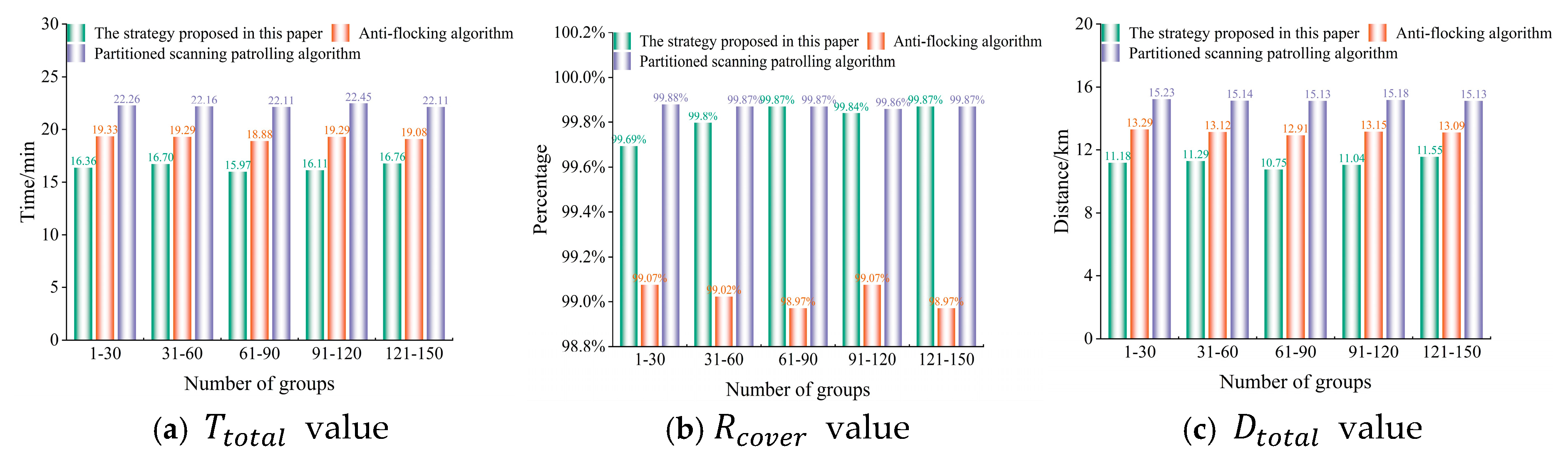
6.2.1. Performance Comparison of Three Algorithms

To validate the effectiveness of the proposed algorithm, comparative experiments were conducted in different task areas with three obstacles. The performance of the proposed Training Framework for Multi-USV (TFMUSV) was benchmarked against two existing algorithms: the anti-flocking algorithm and the partition scanning algorithm. In terms of navigation efficiency, the differences in the performance of the three algorithms are reflected in the three performance parameters: R c o v e r , D t o t a l , and T t o t a l .
As shown in Figure 12, from the rate of increase of the R c o v e r i k value, the proposed TFMUSV is significantly better than both the anti-flocking algorithm and the partition scanning patrol algorithm. At the same time point, the R c o v e r i k 99 % value with the proposed algorithm is higher than that of the other two control algorithms. When the system controlled by the proposed TFMUSV achieves the task goal ( R c o v e r i k 99 % ), the R c o v e r i k values of the anti-flocking algorithm and the partition scanning patrol algorithm are 94.38% and 85.12%, respectively.
As shown in Figure 13, Figure 14 and Figure 15, it can be observed that the proposed TFMUSV consistently has the smallest D t o t a l and T t o t a l values in all task scenarios. Although the R c o v e r values under the algorithm proposed in this paper are slightly lower than those of the partition scanning patrol algorithm in various task scenarios, the R c o v e r i k values still remain above 99%, which is sufficient to meet the predefined task objectives. The proposed TFMUSV demonstrates significant performance improvements, achieving a 23% reduction in T t o t a l and a 25% decrease in D t o t a l compared to the anti-flocking method. When benchmarked against the partition scanning patrol algorithm, the proposed TFMUSV reduces T t o t a l by 74% and D t o t a l by 63%, highlighting its superior efficiency in dynamic path planning and resource optimization.

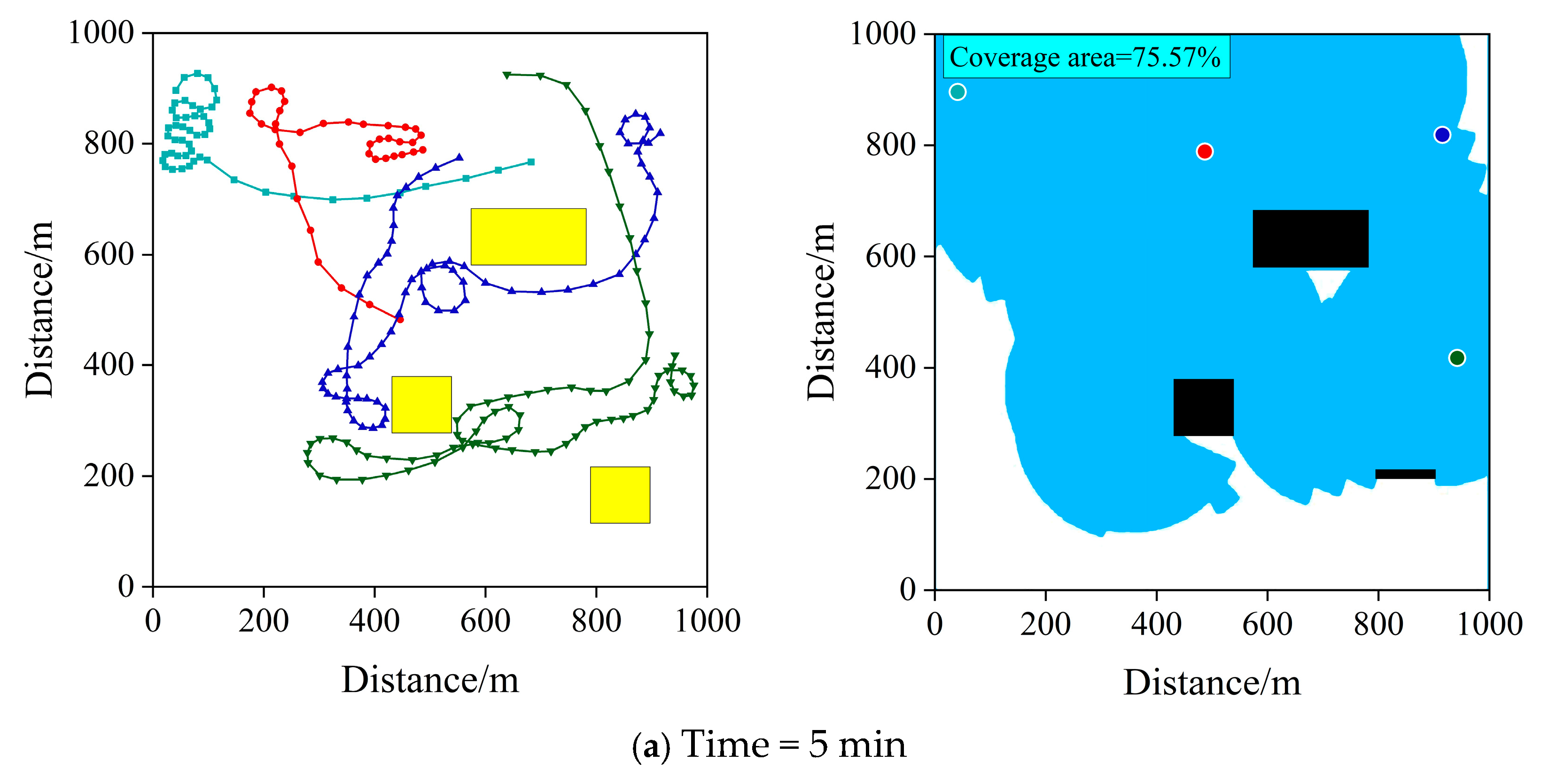
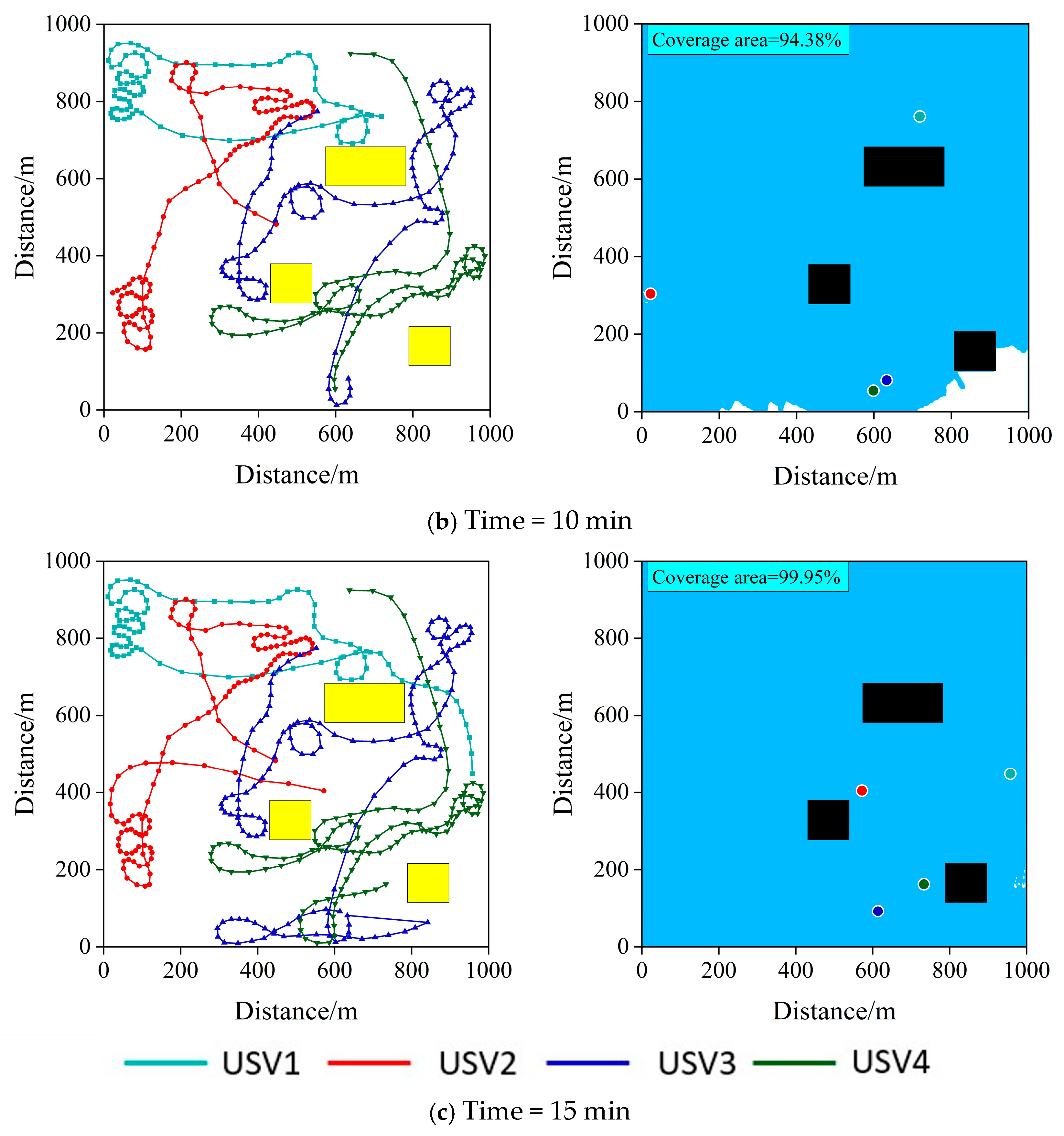
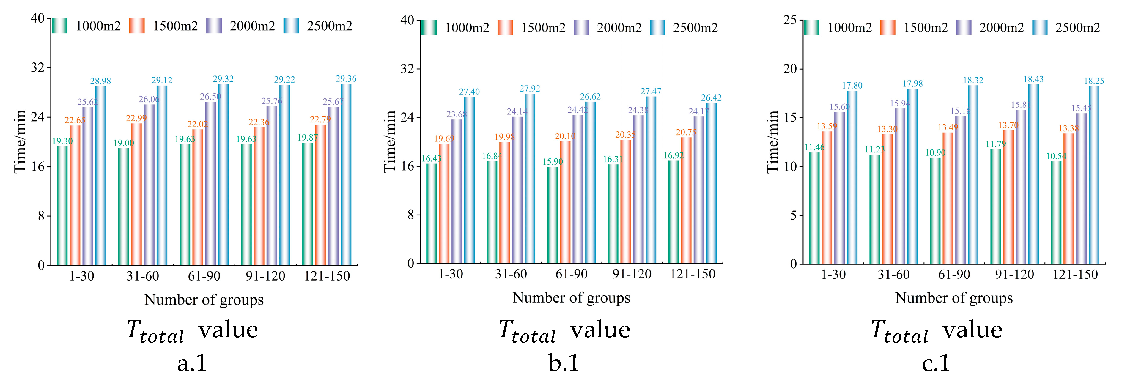
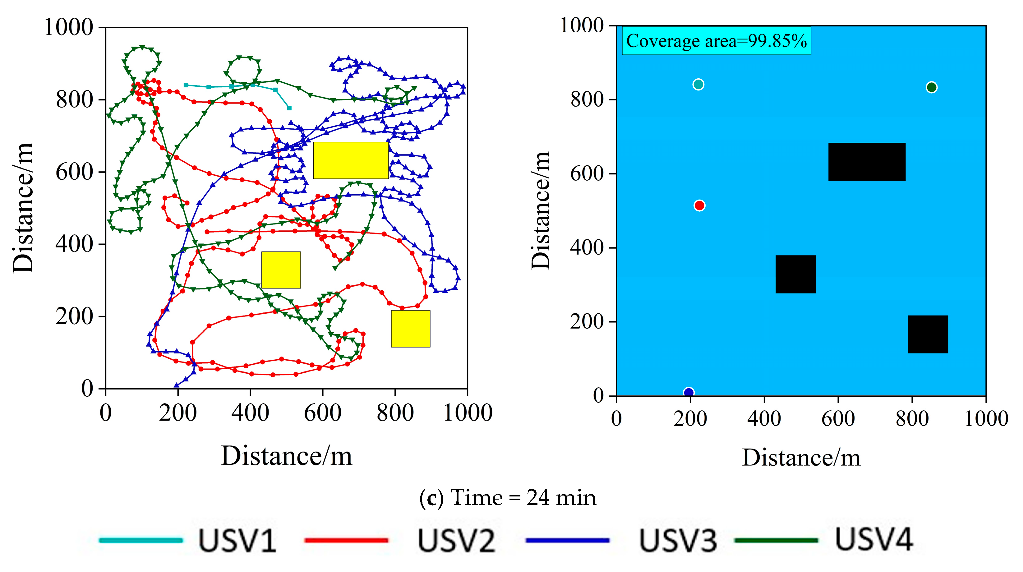
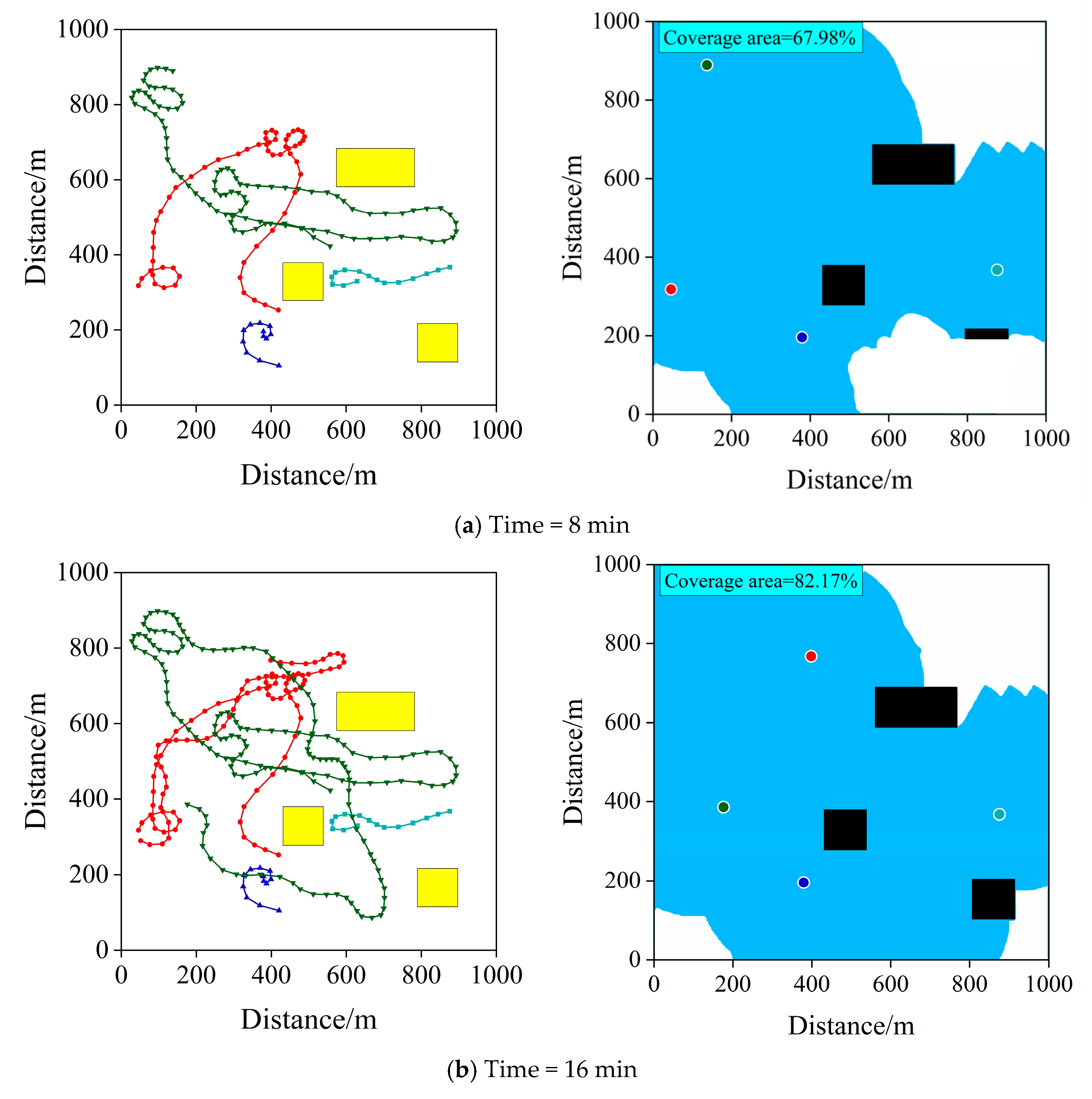
6.2.2. Performance Analysis of the Proposed Algorithm

This section provides a systematic validation of the proposed multi-USV cooperative patrol algorithm, focusing on its core advantages in coverage efficiency, path planning, and dynamic adaptability. Key performance metrics, including R c o v e r , D t o t a l , T t o t a l , CRBAA and CRBAO, are rigorously analyzed. Scalability tests under varying task areas (1–2.5 km2) and communication radius (200–500 m) further validate the algorithm’s robustness in dynamic environments.
As shown in Figure 16, the navigation trajectories under the proposed algorithm exhibit three distinct operational phases. During the initial stage (Figure 16a,b), the overlap ratio of node trajectories remains below 5%, demonstrating efficient resource dispersion enabled by real-time collaborative information graphs (Equation (11)). This design minimizes redundant exploration while maximizing early-stage coverage efficiency. As the mission progresses, nodes gradually disperse to designated operational zones, highlighting the kinematic smoothing effect of dynamic window constraints (Equations (15)–(17)). During the mission, we observed that the navigation trajectories of some nodes exhibited “drastic” unclosed loops near the boundaries of unexplored regions (as shown by the red trajectory in Figure 16). This phenomenon can be attributed to the following factors: First, the feasible velocity vectors (RV) generated by the dynamic window algorithm (Equations (15)–(17)) only consider short-term kinematic constraints and obstacle avoidance requirements, without fully integrating global coverage objectives. This may cause path oscillations or abrupt turns when nodes approach the boundaries of unexplored regions. Second, although dense rewards have been introduced through reward reshaping (Equations (20), (23) and (36)), the gradient of the exploration reward R c o v e r i k may become discontinuous at the boundaries of unexplored regions, triggering “sudden” turns. However, in the final phase (Figure 16c), nodes collectively converge on uncovered regions, which validates the dense reward mechanism’s capability to balance exploration and cooperation (Equation (39)).
The algorithm’s environmental perception accuracy is confirmed by the high-fidelity water depth map in Figure 17. Concurrently, obstacle avoidance performance is evidenced by maintained safety margins in trajectory plots and ultralow collision rates (CRBAA < 0.5%, CRBAO < 0.3%, Figure 18). These outcomes are attributed to the integrated artificial potential field model (Equations (27)–(30)) and obstacle inflation strategy (Equation (35)), which enable proactive collision prevention rather than reactive maneuvers.
As shown in Figure 19 and Figure 20, extended evaluations under scaled task areas (1–2.5 km2) and communication radius (200–500 m) demonstrate the algorithm’s adaptability. Although both the T t o t a l value and D t o t a l increase with the growing task area, the R c o v e r value consistently remains above 99%. Moreover, both the CRBAO and CRBAA values demonstrate that the nodes in the system can ensure safe navigation. This indicates that, even when facing different task areas, the system can still achieve the predefined task objectives under the control of the proposed algorithm.
The patrol performance of the system is influenced by the node communication radius ( R c ). Expanding the communication radius from 200 m to 500 m reduces T t o t a l by 9.3% and D t o t a l by 7.8%. The primary reason for the test results mentioned above is that the variation in R c affects the USV’s ability to update task status information. In other words, a larger R c allows the node to integrate task information from more nodes, making the task information more complete and accurate, which in turn helps generate more effective actions. Test results from different task areas and communication distances indicate that when the task area and system communication radius change, the algorithm in this paper still enables the system to accomplish the task.

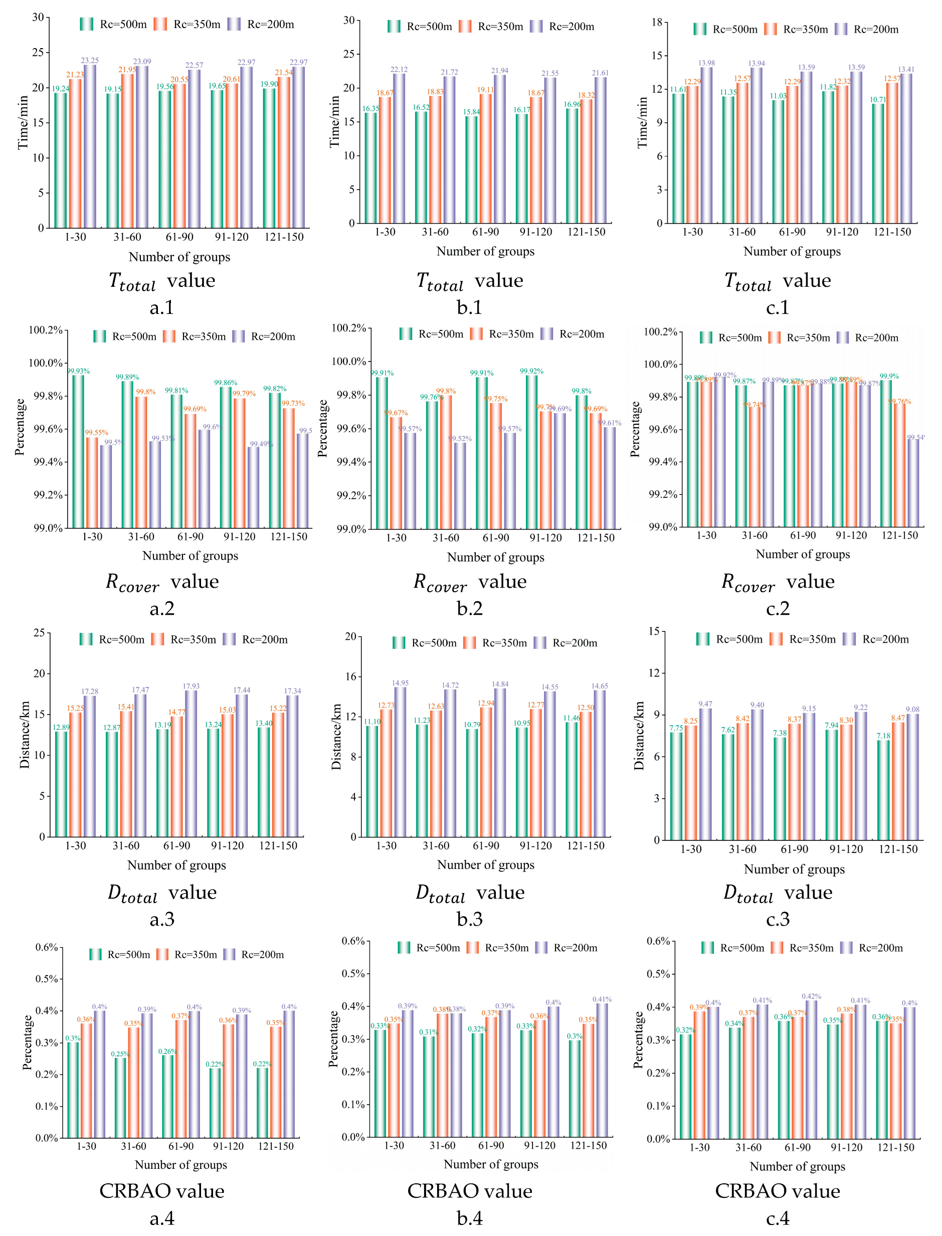
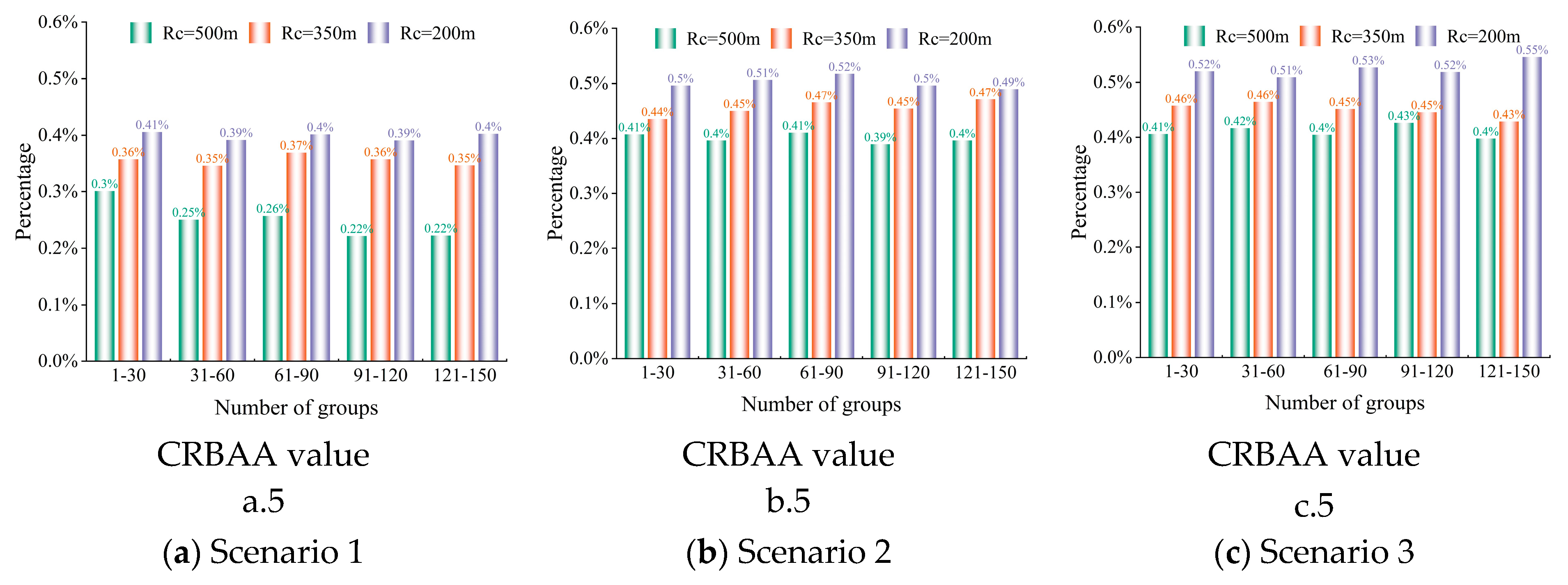
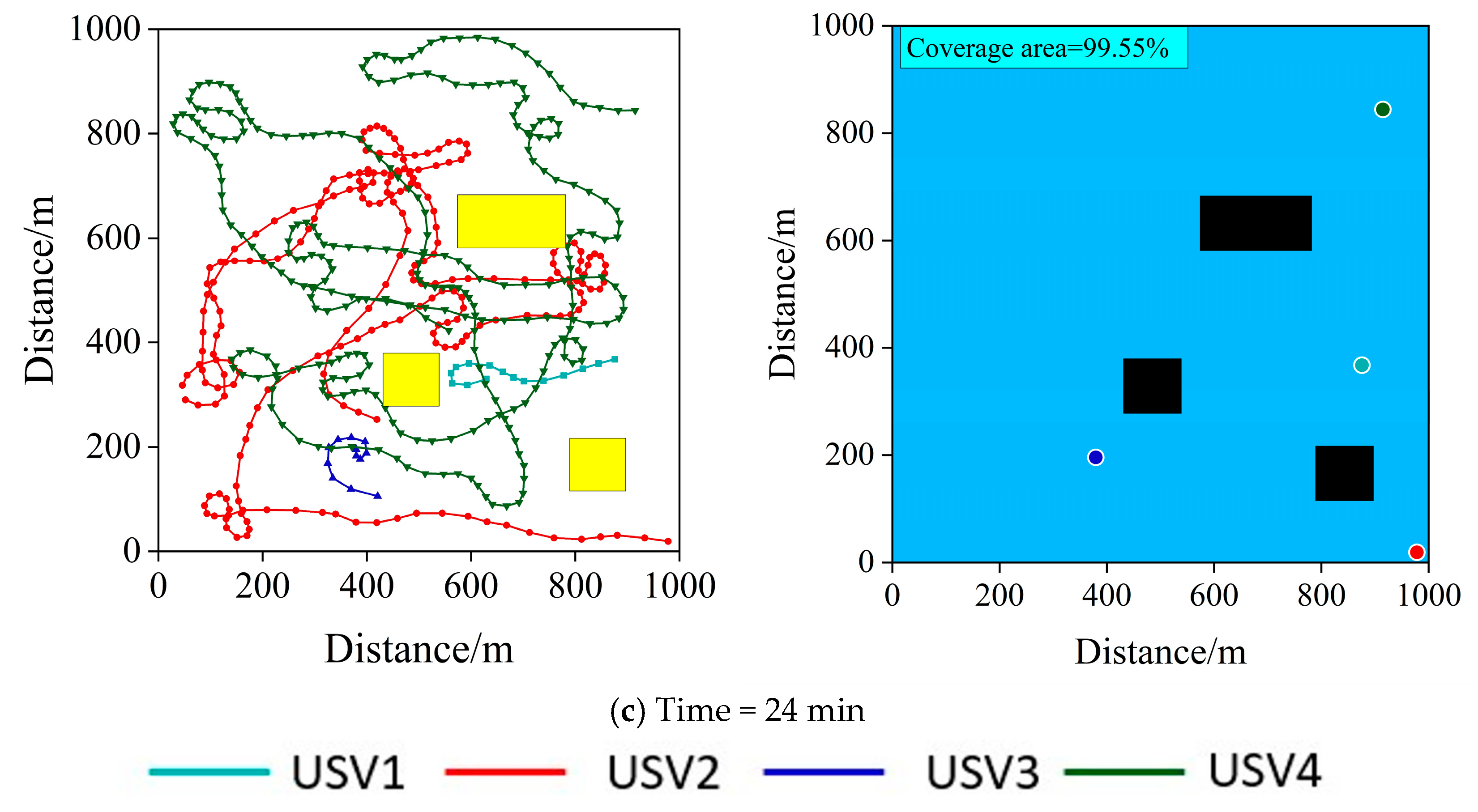
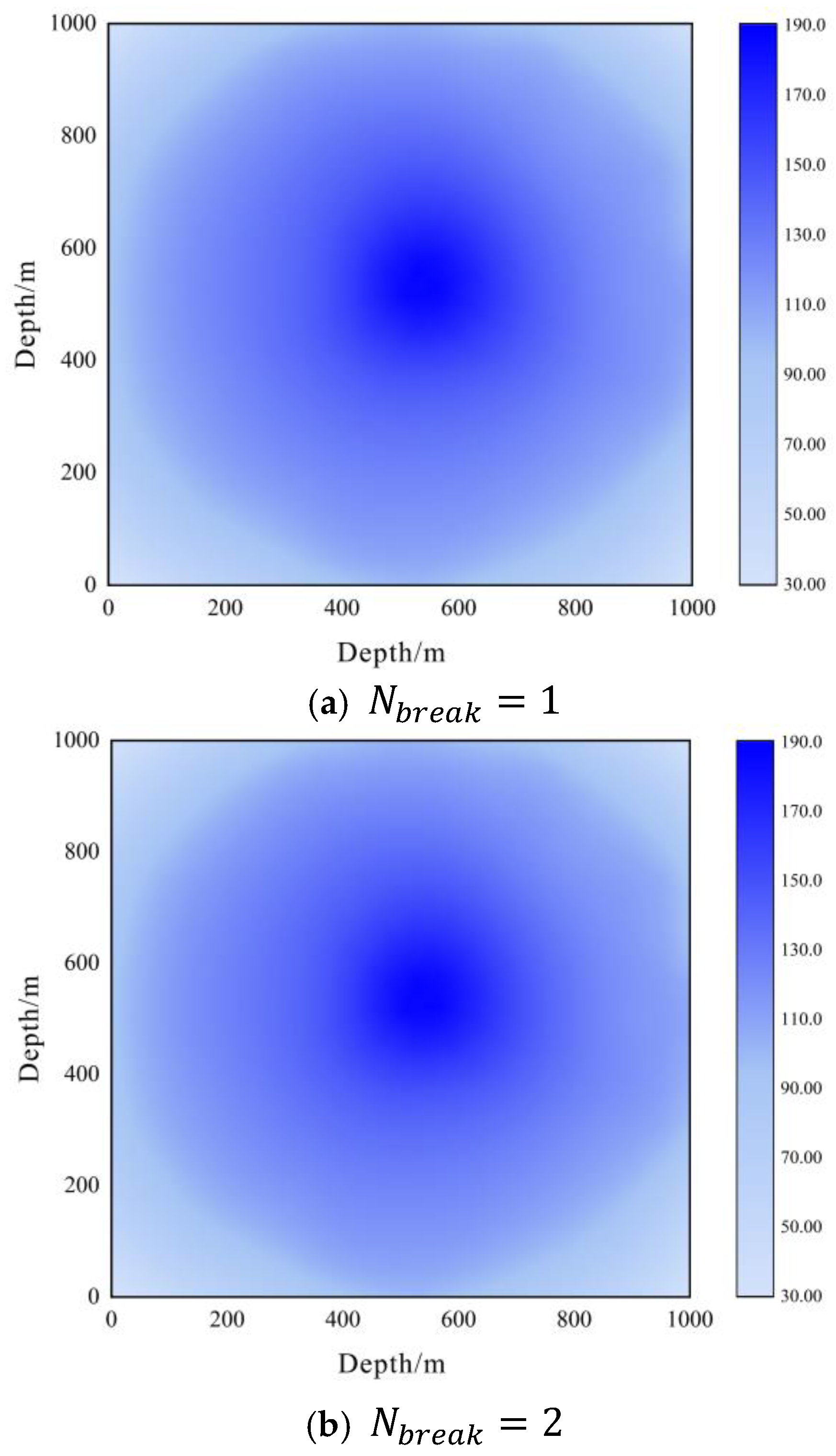
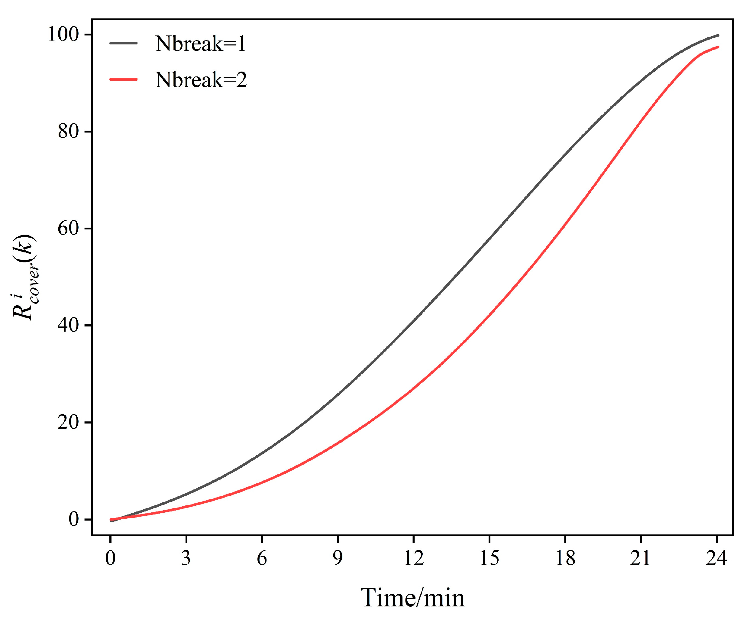
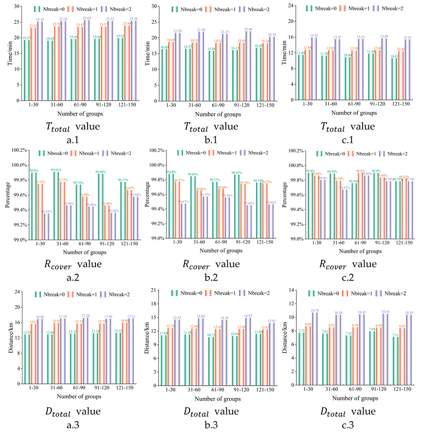
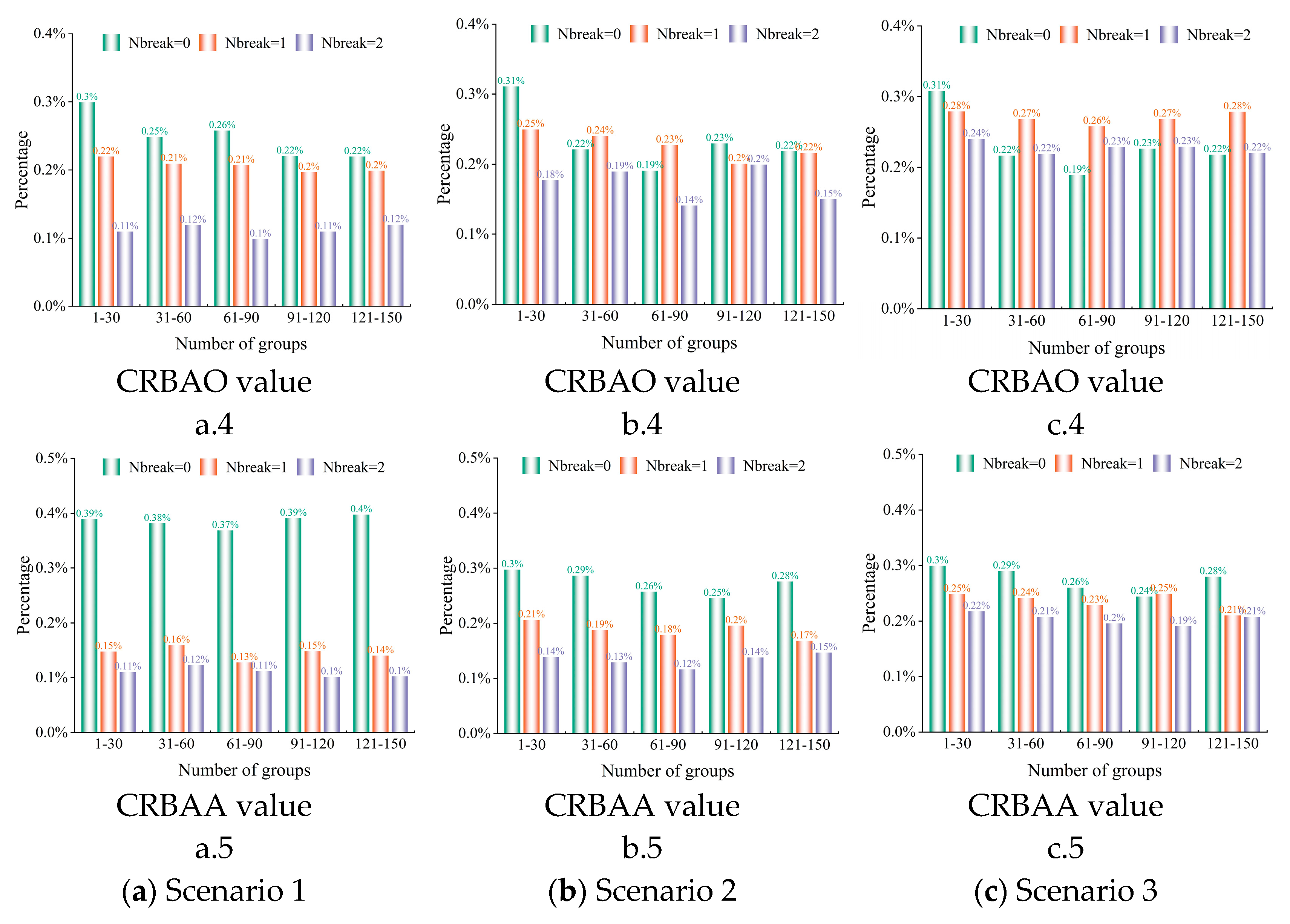
6.3. Robustness Performance Test
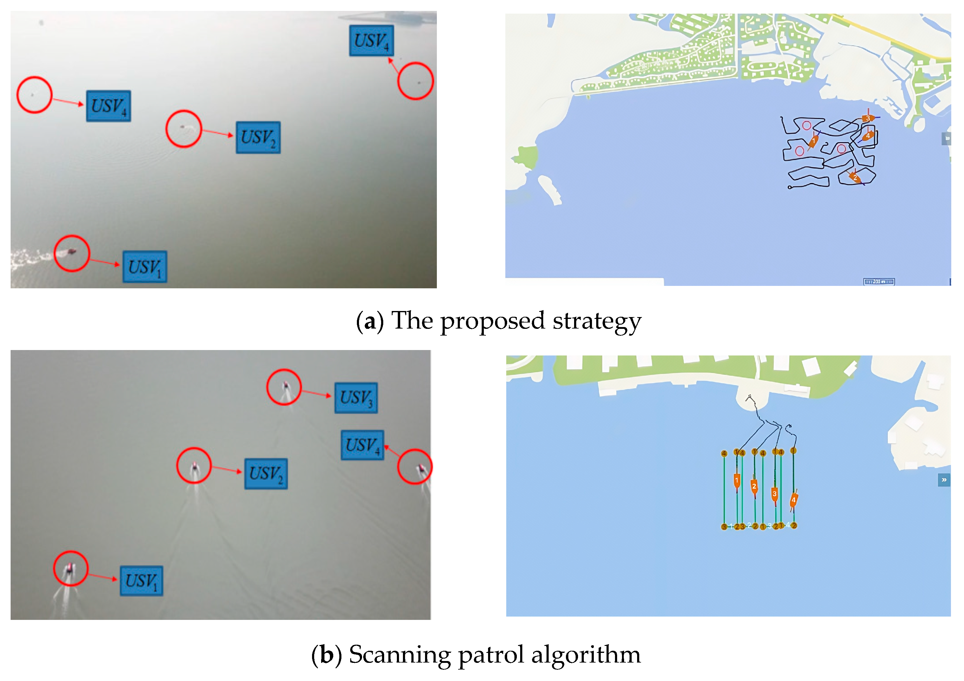
This section will test the robustness performance of the system under the algorithm proposed in this paper. The test task scenario is identical to the task scenario in the previous section’s performance testing. During the test, nodes are randomly selected from the system to act as faulty nodes. Once a node is selected as a faulty node, it will immediately stop operating. The selected faulty nodes will immediately stop their operations. In each test scenario, two different configurations for the number of faulty nodes are considered: N b r e a k = 1 and N b r e a k = 2 .
Due to the limitations in the length of the paper, the analysis will focus on the testing results of Scenario 2. As shown in Figure 21 and Figure 22, the navigation trajectories of each node under the cooperative patrol control algorithm indicate that, during the early stage of the task, as illustrated in Figure 21a and Figure 22a, one or two nodes in the system stopped operations after performing tasks for a period of time. However, it can be observed from Figure 21 and Figure 22 that after some nodes in the system stopped operating, other remaining nodes took over the tasks of the corresponding faulty nodes and covered their originally assigned operational areas during their continued operation. The work process of the remaining nodes is generally consistent with the work process of the nodes in the previous performance test. Although there is some overlap in the operational areas of the four nodes, the overlapping trajectories are minimal. As the task progresses, the navigation trajectories of the four nodes gradually disperse, heading toward their respective areas of operation. In the final segment of the task, all nodes begin to approach areas that still lack patrol information and carry out operations in those areas. Regardless of whether the number of faulty nodes is N b r e a k = 1 or N b r e a k = 2 , the navigation trajectories of the nodes in the system all conform to the aforementioned situation. As shown in Figure 23, the system’s actual acquisition of bathymetric data in the task area under different numbers of faulty nodes demonstrates that the system has successfully obtained the bathymetric data of the task area. This confirms that, under the algorithm proposed in this paper, even in the presence of faulty nodes, the system is still able to complete the set patrol objectives.
The test results of R c o v e r i k in Scenario 2 are shown in Figure 24. By analyzing the changes in R c o v e r i k , it can be observed that the number of N b r e a k has a certain impact on the system’s patrol efficiency. Specifically, in the early stages of the task, the greater the number of N b r e a k , the more significant the impact on the system’s patrol efficiency, resulting in a decrease in the system’s operational efficiency. However, as the task progresses, the influence of faulty nodes on the system’s operational efficiency gradually diminishes, and the performance gap between different numbers of faulty nodes begins to narrow. Nevertheless, this gap still exists by the end of the task. As seen in the results presented in Figure 20, the number of N b r e a k does not have a significant effect on the final R c o v e r i k value. The R c o v e r i k values in all test scenarios still reach over 99%. Figure 25 also presents the variations of several test parameters, including T t o t a l , D t o t a l , R c o v e r , CRBAO, and CRBAA, under different test scenarios. The test results indicate that the algorithm proposed in this paper exhibits strong robustness. When a system node experiences an unexpected failure and can no longer function, the algorithm is still able to provide optimal task actions in real-time based on the current task situation. This minimizes the negative impact of the faulty node on the system’s operations, ensuring the system continues to operate normally with a certain level of operational capability. Furthermore, during the operation, the algorithm ensures the navigational safety of the nodes.

7. Practical Test

7.1. Experimental Scenario

In the cooperative patrol experiment scenario, the base station’s latitude and longitude are (120.876243, 31.079691). A patrol area of 1 km × 1 km is set up within its vicinity, and the task objective is to use a multi-unmanned boat system to collect depth data across the entire mission area. Considering the practical conditions faced by the multi-unmanned boat system and the reliability constraints of the nodes, the real-boat test for the cooperative patrol task is divided into three groups: Experiment 1, with four unmanned boats operating in a task area with four obstacles, without any failure nodes; Experiment 2, with four unmanned boats, in which one failure node occurs (a randomly selected node is instructed to shut down by the shore terminal); Experiment 3, with four unmanned boats, in which two failure nodes occur, in a task area with four obstacles. The scanning patrol algorithm was chosen as the comparison testing algorithm.
To verify the effectiveness of the cooperative patrol control algorithm for the multi-unmanned boat system proposed in this paper, due to actual test conditions, the dynamics and kinematics models of the test boats differ from those used for the simulation experiments. Therefore, in the real-boat test, based on the real-time collective status of the water area, the proposed strategy outputs control actions. After coordinate system alignment and transformation, the control instructions are sent to the decision control system of the unmanned boats. The specific control process is as follows: the current situation (such as the unmanned boats’ coordinates and speed) is transformed into the simulation environment’s coordinate system. The trained task strategy, based on the transformed situation information, outputs the acceleration of the unmanned boats, from which speed and the next time-step coordinates are calculated. These are then converted into latitude, longitude coordinates, and speed in the water area coordinate system. Finally, the waypoint/speed control mode is used to control the unmanned boats’ movement. Due to objective constraints, the sensors carried by the nodes are also simulated or simplified. During the test, the nodes in the system do not carry the sensors needed to detect the depth. Instead, the patrol results of the nodes are provided by the shore-based platform, which constructs the water depth model of the task area and combines it with the real-time position feedback from each node.

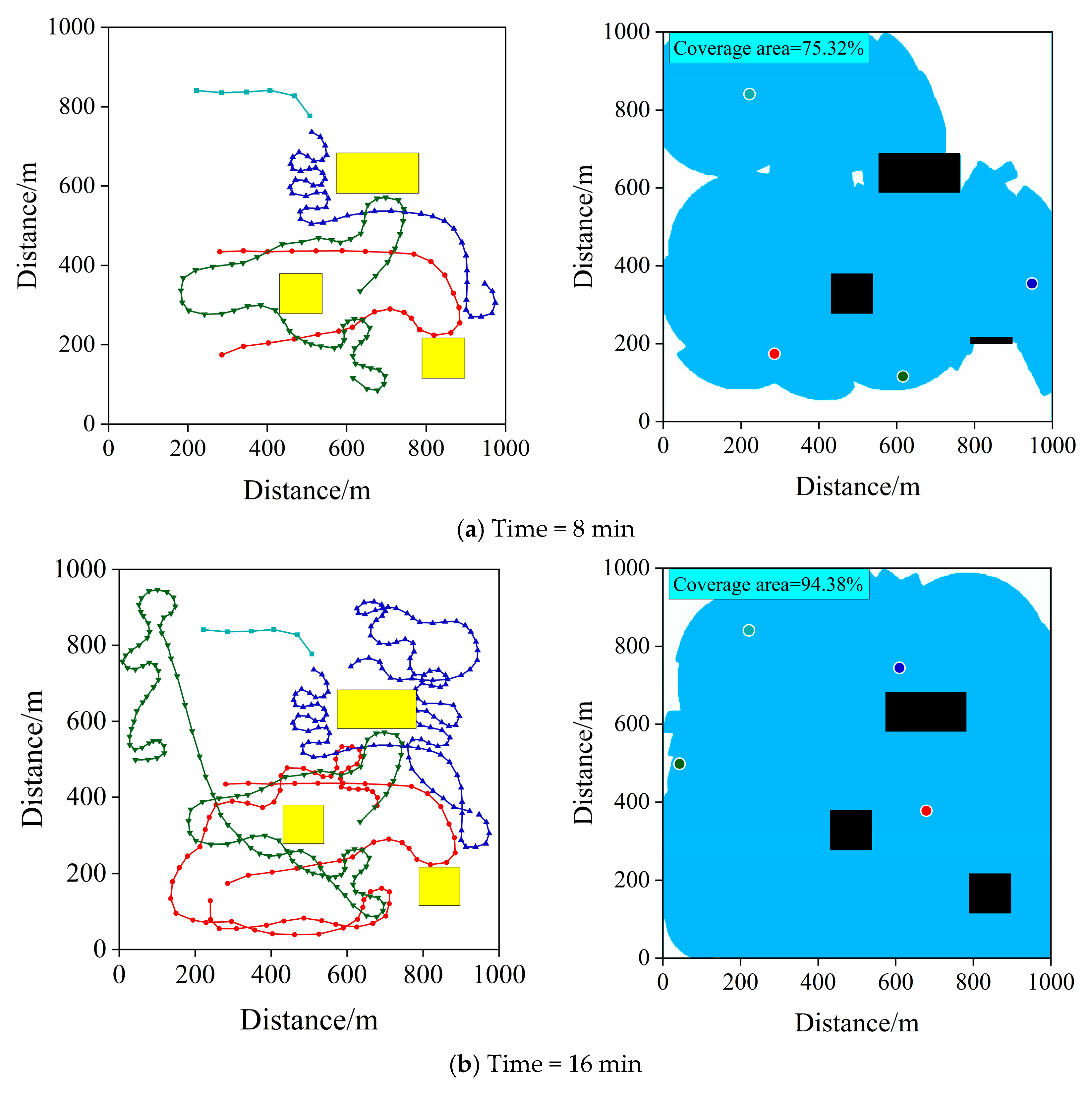
7.2. Experimental Results and Analysis

The test results of Experiment 1 are shown in Figure 26 and Figure 27. The focus is on the test situation under the control of the multi-unmanned boat flexible cooperative patrol control strategy, aimed at global coverage. From the navigation trajectories of the nodes in the test process shown in Figure 26, it can be observed that the navigation trajectories of the nodes are evenly distributed within the task area, and no collisions occurred with the virtual obstacles in the test area. The changes in CRBAA and CRBAO data, as shown in Table 3, also demonstrate that the proposed strategy effectively achieves collision avoidance between nodes as well as between nodes and obstacles, ensuring the safe navigation of the nodes. From the depth map of the task area obtained under the control of the proposed strategy, shown in Figure 27, it can be seen that the system has successfully acquired the water depth data of the entire task area by the end of the mission. By mapping the completeness of depth data acquisition, we indirectly verify the algorithm’s ability to ensure global patrol coverage. In the test, the main differences in performance between the two control algorithms are reflected in the performance parameters T e p i s o d e , R c o v e r , and D t o t a l . Table 3 shows the variations of these test parameters ( T e p i s o d e , D t o t a l , R c o v e r ) under multiple test scenarios. The test results indicate that, compared to the scanning patrol algorithm, the proposed strategy has a similar R c o v e r value, while the D t o t a l and T e p i s o d e values are relatively lower. This suggests that the proposed strategy, in comparison to the scanning patrol algorithm, offers higher patrol efficiency and enables the system to effectively complete the cooperative patrol mission.
The test results of Experiment 2 and Experiment 3 are shown in Figure 28. From the test results, it can be seen that after certain nodes in the system stop working, other nodes continue to operate and take over the patrol tasks in the nearby task areas of the failed nodes. The navigation trajectories of the remaining nodes are evenly distributed within the task area. Table 4 shows the variation of test parameters T e p i s o d e , D t o t a l , and R c o v e r under multiple tests. It can be observed that the number of N b r e a k and the time when a node fails mainly affect the system’s patrol efficiency. The larger the number of N b r e a k , and the earlier the occurrence of a failed node, the larger the value of T t o t a l . However, the tests indicate that the number of N b r e a k and the time of node failure have no significant impact on the final values of R c o v e r , CRBAA, and CRBAO. The system’s coverage of the task area remains above 99%. The test results demonstrate that the proposed strategy is robust, ensuring the system continues to operate normally and maintains a certain level of operational capability even when a node experiences a sudden failure and can no longer function.

8. Conclusions and Future Works

This paper conducts an in-depth study on the cooperative patrol tasks of multi-USV systems. The research first proposes a hybrid embedded task state information modeling method. Based on this, a distributed global collaboration patrol algorithm for multi-USV systems aimed at full-area coverage is proposed, integrating an end-to-end improved OODA decision-making model. By integrating patrol, collaboration, and obstacle information graphs into a unified state representation, the proposed algorithm enables real-time generation of kinematically feasible control actions via dynamic window constraints. The dense reward structure with adaptive weighting coefficients addresses sparse feedback challenges, demonstrating 99.75% coverage rates in simulations and field tests while maintaining collision rates below 0.5%. Experimental validations confirm the framework’s robustness, sustaining operational capability when 50% of nodes malfunction.
Despite these advancements, limitations persist in handling complex hydrodynamic interactions and ultra-large fleet scalability. Future work will focus on integrating environmental current models and wind field estimators to enable real-time compensation for multi-scale disturbances, particularly for typhoon-level winds. And the LSTM-based cooperative information graph demonstrates adaptability in moderate-delay scenarios, its performance under significant communication delays ( t > 2 s) remains an open challenge. Future work will integrate delay-tolerant mechanisms, such as hybrid Kalman-filter-LSTM prediction and decentralized clock synchronization protocols, to enhance real-time coordination in latency-prone environments. Empirical validation under controlled delay injection will be conducted to quantify the framework’s robustness.
This research establishes a theoretical and practical foundation for autonomous maritime surveillance systems, offering scalable solutions for environmental monitoring and search-rescue missions. The proposed methodology bridges the gap between reinforcement learning theory and marine robotics applications, paving the way for intelligent coordination in complex oceanic scenarios.

Author Contributions

Conceptualization, Y.L.; Data curation, X.X.; Formal analysis, L.L.; Funding acquisition, Y.L.; Investigation, Y.X.; Methodology, Y.L.; Project administration, Y.X.; Resources, L.L.; Software, G.L. and Y.G.; Supervision, Y.L. and W.S.; Validation, X.X. and G.L.; Visualization, Y.L. and Y.G.; Writing—original draft, Y.L.; Writing—review & editing, X.X. All authors have read and agreed to the published version of the manuscript.

Funding

This work was supported in part by Anhui Provincial University Research Plan Project 2024AH050613, in part by Anhui Xinhua University’s 2023 Campus level Natural Science Project 2023zr004, in part by Anhui Province Higher Education Quality Engineering Project 2023xjzlts087, in part by Anhui Xinhua University Higher Education Quality Engineering Project 2023sdxxj02.

Data Availability Statement

The original contributions presented in this study are included in the article. Further inquiries can be directed to the corresponding author.

Conflicts of Interest

The authors declare there are no conflicts of interest regarding the publication of this paper.

References

  1. Zhu, D.; Pan, Y.J. Optimal Motion Planning for Heterogeneous Multi-USV Systems Using Hexagonal Grid-Based Neural Networks and Parallelogram Law Under Ocean Currents. IEEE Trans. Syst. Man Cybern. Syst. 2025, 55, 43–50. [Google Scholar] [CrossRef]
  2. Chen, T.; Peng, H.; Chang, X.; Zhang, X.; Wang, D. Co-Design of USV Control System Based on Fuzzy Satisfactory Optimization for Automatic Target Arriving and Berthing. IEEE Access 2024, 12, 102449–102460. [Google Scholar] [CrossRef]
  3. Guo, X.; Narthsirinth, N.; Zhang, W.; Hu, Y. Unmanned Surface Vehicles (USVs) Scheduling Method by a Bi-Level Mission Planning and Path Control. Comput. Oper. Res. 2024, 162, 106472. [Google Scholar] [CrossRef]
  4. Xu, Y.; Li, K.; Li, Y. Distributed Optimal Control of Nonlinear Multi-Agent Systems Based on Integral Reinforcement Learning. Optim. Control Appl. Methods 2024, 172, 104321. [Google Scholar] [CrossRef]
  5. Marchukov, Y.; Montano, L. Occupation-aware planning method for robotic monitoring missions in dynamic environments. Robot. Auton. Syst. 2025, 185, 104892. [Google Scholar] [CrossRef]
  6. Gao, S.; Peng, Z.; Wang, H.; Liu, L.; Wang, D. Long Duration Coverage Control of Multiple Robotic Surface Vehicles Under Battery Energy Constraints. IEEE/CAA J. Autom. Sin. 2024, 11, 1695–1698. [Google Scholar] [CrossRef]
  7. Zhao, L.; Bai, Y.; Paik, J.K. Optimal Coverage Path Planning for USV-Assisted Coastal Bathymetric Survey: Models, Solutions, and Lake Trials. Ocean Eng. 2024, 296, 116921. [Google Scholar] [CrossRef]
  8. Zhao, L.; Bai, Y. Energy Efficient Coverage Path Planning for USV-Assisted Inland Bathymetry Under Current Effects: An Analysis on Sweep Direction. Ocean Eng. 2024, 305, 117910. [Google Scholar] [CrossRef]
  9. Zhao, L.; Bai, Y. Joint-Optimized Coverage Path Planning Framework for USV-Assisted Offshore Bathymetric Mapping: From Theory to Practice. Knowl.-Based Syst. 2024, 304, 112449. [Google Scholar] [CrossRef]
  10. Garg, A.; Jha, S.S. Learning Continuous Multi-UAV Controls with Directed Explorations for Flood Area Coverage. Robot. Auton. Syst. 2024, 180, 104774. [Google Scholar] [CrossRef]
  11. Wang, S.; Zhu, D.; Zhou, C.; Sun, G. Improved Grey Wolf Algorithm Based on Dynamic Weight and Logistic Mapping for Safe Path Planning of UAV Low-Altitude Penetration. J. Supercomput. 2024, 80, 25818–25852. [Google Scholar] [CrossRef]
  12. Novak, D.; Tebbani, S.; Goricanec, J.; Orsag, M.; Le Brusquet, L. Battery Management Optimization for an Energy-Aware UAV Mapping Mission Path Planning. In Proceedings of the 2024 10th International Conference on Control, Decision and Information Technologies (CoDIT), Vallette, Malta, 1–4 July 2024; pp. 2645–2650. [Google Scholar]
  13. Vashisth, A.; Patel, D.; Conover, D.; Bera, A. Multi-Robot Informative Path Planning for Efficient Target Mapping Using Deep Reinforcement Learning. arXiv 2024, arXiv:2409.16967. [Google Scholar]
  14. Pérez-González, A.; Benítez-Montoya, N.; Jaramillo-Duque, Á.; Cano-Quintero, J.B. Coverage Path Planning with Semantic Segmentation for UAV in PV Plants. Appl. Sci. 2021, 11, 12093. [Google Scholar] [CrossRef]
  15. Wang, Y.; Xi, M.; Weng, Y. Intelligent Path Planning Algorithm of Autonomous Underwater Vehicle Based on Vision Under Ocean Current. Expert Syst. 2025, 42, e13399. [Google Scholar] [CrossRef]
  16. Gupta, S.; Kumar, A.; Kumar, V.; Singh, S.; Gautam, M. Autonomous Underwater Vehicle Path Planning Using Fitness-Based Differential Evolution Algorithm. J. Comput. Sci. 2025, 85, 102498. [Google Scholar] [CrossRef]
  17. Soleymani, F.; Miah, M.S.; Spinello, D. Optimal Non-Autonomous Area Coverage Control with Adaptive Reinforcement Learning. Eng. Appl. Artif. Intell. 2023, 122, 106068. [Google Scholar] [CrossRef]
  18. Papatheodorou, S.; Stergiopoulos, Y.; Tzes, A. Distributed Area Coverage Control with Imprecise Robot Localization. In Proceedings of the 2016 24th Mediterranean Conference on Control and Automation (MED), Athens, Greece, 21–24 June 2016; pp. 214–219. [Google Scholar]
  19. Yu, J.; Mi, R.; Han, J.; Yang, W. Voronoi-Based Adaptive Area Optimal Coverage Control for Multiple Manipulator Systems with Uncertain Kinematics and Dynamics. Commun. Nonlinear Sci. Numer. Simul. 2024, 138, 108235. [Google Scholar] [CrossRef]
  20. Magalhães, A.C.; Raffo, G.V.; Pimenta, L.C.A. Safe Voronoi-Based Coverage Control for Multi-Robot Systems with Constraints. In Proceedings of the 2023 Latin American Robotics Symposium (LARS), 2023 Brazilian Symposium on Robotics (SBR), and 2023 Workshop on Robotics in Education (WRE), Salvador, Brazil, 9–11 October 2023; pp. 188–193. [Google Scholar]
  21. Hazon, N.; Kaminka, G.A. Redundancy, Efficiency and Robustness in Multi-Robot Coverage. In Proceedings of the 2005 IEEE International Conference on Robotics and Automation, Barcelona, Spain, 18–22 April 2005; pp. 735–741. [Google Scholar]
  22. Ozkahraman, O.; Ogren, P. Combining Control Barrier Functions and Behavior Trees for Multi-Agent Underwater Coverage Missions. In Proceedings of the 2020 59th IEEE Conference on Decision and Control (CDC), Jeju, Republic of Korea, 14–18 December 2020; pp. 5275–5282. [Google Scholar]
  23. Hyatt, P.; Brock, Z.; Killpack, M.D. A Versatile Multi-Robot Monte Carlo Tree Search Planner for On-Line Coverage Path Planning. arXiv 2020, arXiv:2002.04517. [Google Scholar]
  24. Dong, W.; Liu, S.; Ding, Y.; Sheng, X.; Zhu, X. An Artificially Weighted Spanning Tree Coverage Algorithm for Decentralized Flying Robots. IEEE Trans. Autom. Sci. Eng. 2020, 17, 1689–1698. [Google Scholar] [CrossRef]
  25. Xu, R.; Yao, S.; Gouhe, W.; Zhao, Y.; Huang, S. A Spanning Tree Algorithm with Adaptive Pruning with Low Redundancy Coverage Rate. Comput. Ind. Eng. 2023, 186, 109745. [Google Scholar] [CrossRef]
  26. Kim, S.; Lin, R.; Coogan, S.; Egersted, M. Area Coverage Using Multiple Aerial Robots With Coverage Redundancy and Collision Avoidance. IEEE Control Syst. Lett. 2024, 8, 610–615. [Google Scholar] [CrossRef]
  27. Chen, Z.; Zhou, Z.; Wang, S.; Li, J.; Kan, Z. Fast Temporal Logic Mission Planning of Multiple Robots: A Planning Decision Tree Approach. IEEE Robot. Autom. Lett. 2024, 9, 6146–6153. [Google Scholar] [CrossRef]
  28. Lu, W.; Xiong, H.; Zhang, Z.; Hu, Z.; Wang, T. Scalable Optimal Formation Path Planning for Multiple Interconnected Robots via Convex Polygon Trees. J. Intell. Robot. Syst. 2023, 109, 63. [Google Scholar] [CrossRef]
  29. Zhu, L.; Cheng, J.; Zhang, H.; Zhang, W.; Liu, Y. Multi-Robot Environmental Coverage With a Two-Stage Coordination Strategy via Deep Reinforcement Learning. IEEE Trans. Intell. Transp. Syst. 2024, 25, 5022–5033. [Google Scholar] [CrossRef]
  30. Gosrich, W.; Mayya, S.; Li, R.; Paulos, J.; Yim, M.; Ribeiro, A.; Kumar, V. Coverage Control in Multi-Robot Systems via Graph Neural Networks. arXiv 2021, arXiv:2109.15278. [Google Scholar]
  31. Stolfi, D.H.; Brust, M.R.; Danoy, G.; Bouvry, P. A Cooperative Coevolutionary Approach to Maximise Surveillance Coverage of UAV Swarms. In Proceedings of the 2020 IEEE 17th Annual Consumer Communications & Networking Conference (CCNC), Las Vegas, NV, USA, 10–13 January 2020; pp. 1–6. [Google Scholar]
  32. Xin, B.; Wang, H.; Li, M. Multi-Robot Cooperative Multi-Area Coverage Based on Circular Coding Genetic Algorithm. J. Adv. Comput. Intell. Intell. Inform. 2023, 27, 1183–1191. [Google Scholar] [CrossRef]
  33. Nemer, I.A.; Sheltami, T.R.; Mahmoud, A.S. A Game Theoretic Approach of Deployment a Multiple UAVs for Optimal Coverage. Transp. Res. Part A Policy Pract. 2020, 140, 215–230. [Google Scholar] [CrossRef]
Figure 1. Different decomposition methods for the task area. (a) exact-approximate cell decomposition methods. (b) approximate cell decomposition methods.
Jmse 13 00584 g001
Figure 2. Exact-approximate cell decomposition method. (a) Trapezoidal decomposition method. (b) Cow-plowing-style cell decomposition method.
Jmse 13 00584 g002
Figure 3. Voronoi partitioning and its properties. (a) Voronoi region decomposition. (b) Voronoi region properties.
Jmse 13 00584 g003
Figure 4. Multi-robot spanning tree method. (a) Example of the MSTC method. (b) Examples of different spanning tree methods.
Jmse 13 00584 g004
Figure 5. Patrol information in the task area.
Jmse 13 00584 g005
Figure 6. Obstacle information extraction.
Jmse 13 00584 g006
Figure 7. Discrete velocity vector.
Jmse 13 00584 g007
Figure 8. Training Framework for Multi-USV.
Jmse 13 00584 g008
Figure 9. Training task area.
Jmse 13 00584 g009
Figure 10. Training results using different training algorithms.
Jmse 13 00584 g010
Figure 11. Training results of three algorithms using different combinations of F-weight coefficients.
Jmse 13 00584 g011
Figure 12. The variation value of R c o v e r i k under different control algorithms.
Jmse 13 00584 g012
Figure 13. Performance comparison of test results in Scenario 1.
Jmse 13 00584 g013
Figure 14. Performance comparison of test results in Scenario 2.
Jmse 13 00584 g014
Figure 15. Performance comparison of test results in Scenario 3.
Jmse 13 00584 g015
Figure 16. The navigation trajectory (left panel) and positional distributions (right panel) of each node under the proposed strategy in this paper.
Jmse 13 00584 g016aJmse 13 00584 g016b
Figure 17. The water depth distribution map of the task area obtained by the system under the algorithm proposed in this paper.
Jmse 13 00584 g017
Figure 18. The changes in CRBAA and CRBAO values of the system under the strategy proposed in this paper.
Jmse 13 00584 g018
Figure 19. Strategy performance test results under different task area sizes.
Jmse 13 00584 g019aJmse 13 00584 g019b
Figure 20. Strategy performance test results under different communication conditions.
Jmse 13 00584 g020aJmse 13 00584 g020b
Figure 21. When N b r e a k = 1 , the navigation trajectory (left panel) and positional distributions (right panel) of each node in the system.
Jmse 13 00584 g021aJmse 13 00584 g021b
Figure 22. When N b r e a k = 2 , the navigation trajectory (left panel) and positional distributions (right panel) of each node in the system.
Jmse 13 00584 g022aJmse 13 00584 g022b
Figure 23. The actual water depth distribution map of the task area obtained by the system under the strategy proposed in this paper.
Jmse 13 00584 g023
Figure 24. The changes in the R c o v e r value during testing.
Jmse 13 00584 g024
Figure 25. Performance of the proposed algorithm across scenarios.
Jmse 13 00584 g025aJmse 13 00584 g025b
Figure 26. The navigation scenarios and trajectories of each node under different control strategies employed by the system.
Jmse 13 00584 g026
Figure 27. Actual test results of the patrol strategy proposed in this paper. (a) The changes in navigation parameters of each node during the test process when the system adopts the proposed strategy. (b) The water depth distribution map of the task area acquired by the system.
Jmse 13 00584 g027
Figure 28. The actual vessel test results of the patrol strategy’s robustness in this paper. (a) The navigation trajectories of each node in the system when N b r e a k = 1 and N b r e a k = 2 . (b) The variation of navigation parameters of each node in the system during the test process when N b r e a k = 2 .
Jmse 13 00584 g028
Table 1. Training hyperparameters.
Training HyperparametersValue
Batch1024
Experience replay buffer D 106
Discount factor γ 0.95
Learning rate η 0.01
R s 100 m
R c 500 m
Max episode20,000
Total episode1 × 107
Table 2. Weight series combination.
ABCDEF
β exploration 0.350.350.430.460.480.25
β c o o p e r a t i o n 0.430.390.310.350.510.28
β a v o i d   c o l l i s i o n 0.390.430.450.510.440.51
β e f f i c i e n c y 0.310.410.280.480.350.50
Table 3. Actual vessel test results of the patrol strategy proposed in this paper.
Test Algorithm T e p i s o d e D t o t a l R c o v e r CRBAACRBAO
The proposed strategy in this paper9.5 min1.7 km99.75%0.15%0.00%
Scanning patrol algorithm18.8 min3.3 km100%0.000.00%
Table 4. The actual vessel test results of the patrol strategy’s robustness in this paper.
The Number of Faulty Nodes T t o t a l ,   D t o t a l ,   R c o v e r , CRBAA, CRBAO
N b r e a k = 1
N b r e a k = 2
13.5 min, 8 km, 99.96%, 0.48%, 0.94%, 99.96%
14.9 min, 9 km, 99.94%, 0.44%, 0.41%, 99.69%
Disclaimer/Publisher’s Note: The statements, opinions and data contained in all publications are solely those of the individual author(s) and contributor(s) and not of MDPI and/or the editor(s). MDPI and/or the editor(s) disclaim responsibility for any injury to people or property resulting from any ideas, methods, instructions or products referred to in the content.

