Sea Surface Floating Small-Target Detection Based on Dual-Feature Images and Improved MobileViT

Abstract

Small-target detection in sea clutter is a key challenge in marine radar surveillance, crucial for maritime safety and target identification. This study addresses the challenge of weak feature representation in one-dimensional (1D) sea clutter time-series analysis and suboptimal detection performance for sea surface small targets. A novel dual-feature image detection method incorporating an improved mobile vision transformer (MobileViT) network is proposed to overcome these limitations. The method converts 1D sea clutter signals into two-dimensional (2D) fused images by means of a Gramian angular difference field (GADF) and recurrence plot (RP), enhancing the model’s key-information extraction. The improved MobileViT architecture enhances detection capabilities through multi-scale feature fusion with local–global information interaction, integration of coordinate attention (CA) for directional spatial feature enhancement, and replacement of ReLU6 with SiLU activation in MobileNetV2 (MV2) modules to boost nonlinear representation. Experimental results on the IPIX dataset demonstrate that dual-feature images outperform single-feature images in detection under a ${10}^{-3}$ constant false-alarm rate (FAR) condition. The improved MobileViT attains 98.6% detection accuracy across all polarization modes, significantly surpassing other advanced methods. This study provides a new paradigm for time-series radar signal analysis through image-based deep learning fusion.

1. Introduction

As a crucial technology for small-target detection on the sea surface, radar facilitates the all-weather and long-distance monitoring of sea surface targets by transmitting, propagating, and reflecting electromagnetic waves. Being nonlinear and complex, sea clutter signals vary in different maritime environments due to their non-Gaussian and non-smooth characteristics. A low signal-to-clutter ratio (SCR) and detection leakage often result from target signal obliteration. In addition, the multipath effect and strong sea clutter generated in high sea states often cause false alarms, further complicating the detection process.

Traditional approaches for small-target detection are typically based on statistical theory, as well as on fractal and chaotic properties. Statistical theory creates a model for sea clutter amplitude measurement, but it is often complicated and not widely applicable. In addition, it does not include natural sea clutter dynamics. Research on fractal and chaotic properties remains at the theoretical stage, as it attracts a high cost in terms of fractal dimensions, embedding dimensions, and time delays. Recent studies revealed that a variety of features can be extracted from sea surface clutter and target signals and then differentiated. Based on a non-additive model, Shi et al. [1] proposed a joint feature detection algorithm to transform the detection into a binary classification by combining the convex packet algorithm with the obtained discriminative regions. Based on the convex packet algorithm, Shui et al. [2] developed a three-feature detector based on three types of features extracted from a sea clutter time series, delivering a significant detection performance improvement. The authors subsequently proposed their target return enhancement algorithm, based on the standardized smoothed pseudo-Wigner–Ville distribution (SPWVD) in the time–frequency domain [3]. With this algorithm, the team constructed a three-dimensional (3D) feature vector using the ridge integral and the connectivity region features in a binary image. A classifier constructed from the resulting vector was then trained on sea clutter wave samples, and the classifier effectively controlled the false-alarm rate (FAR), reaching a further enhanced detection performance. In subsequent research, an ever-increasing number of features in detectors have been proposed, reaching a current total of eight. For example, Suo et al. [4] added two new features to their previous six and constructed an eight-feature anomaly detector based on a principal component analysis. However, despite achieving an improved detection accuracy, combining these features leads to potential feature redundancy and increased computation time.

In addition, detection methods containing images have emerged as a hot research issue. Yao et al. [5] proposed an algorithm for floating small-target detection on the sea surface, based on graph connectivity density (GCD). Xu et al. [6] considered the amplitude correlation in the frequency domain between echo data in the feature detection. Despite its novelty in image processing, the feature extraction itself and the detection accuracy were deemed unsatisfactory, leading to the emergence of another approach.

AI-related techniques also find application in sea clutter target detection. Traditional machine learning methods mainly adopt support vector machines (SVMs), random forests, principal component analyses (PCAs), k-nearest neighbors (KNN), and simple neural networks. However, their noise and interference sensitivity hinders their learning of complex sea clutter signals. In comparison, deep learning (DL) networks can achieve good results in tasks involving prediction, classification, and detection, convolutional neural networks (CNNs), recurrent neural networks (RNNs), and long short-term memory networks (LSTMs), to name just a few examples. These approaches typically demand large amounts of data.

Considering the complexity of the data, the detection method combining images and deep learning stands out. Chen et al. [7] first performed a Gramian angular field (GAF) transformation on time-series signals, and then trained a CNN [8] on the resultant images to improve their candlestick morphology recognition accuracy. Similarly, a GAF operation in the study of Toma et al. [9] first converted bearing fault signals into images and classified faults in combination with a CNN. Being merely efficient in capturing local image features, a classical CNN cannot competently identify relationships among distant parts in an image. In 2020, the emergence of the vision transformer (ViT) [10] inaugurated a new era in image processing. The ViT divides images into patches and maps them into sequences, leveraging the self-attention mechanism of the Transformer to model the global relationships among image patches, thus achieving remarkable results. Subsequently, researchers began to explore the advantages of combining CNNs and ViTs, giving rise to a series of hybrid models [11,12,13,14]. While these models have achieved improved performance to some extent, there is still room for the development of lightweight, high-performance visual models for mobile devices. The advent of the mobile vision transformer (MobileViT) [15] marked a significant milestone, innovatively integrating the characteristics of CNNs and ViTs, thereby substantially enhancing the model performance while maintaining a lightweight architecture. Zheng et al. [16] employed the MobileViT neural network for the real-time classification of clustered constellation images, and the experimental results demonstrated the superiority and efficiency of MobileViT. Similarly, Jiang et al. [17] utilized MobileViT and improved the inverted residual structure within the network, thereby increasing the accuracy of facial expression recognition.

Nowadays, with the mature development of deep learning technology, modular design has emerged as an effective strategy to enhance the efficiency and flexibility of models. Through task decomposition, the modular approach can break down complex problems into more manageable subtasks, thereby improving the computational efficiency and scalability of the model. In tasks such as image processing, feature extraction, and image detection, block-based network structures and hybrid modular structures can significantly improve the model’s performance. For example, Wang et al. [18] proposed a multi-label fundus image classification ensemble model based on cellular neural networks. This model adopts a block-combined network structure, consisting of an EfficientNet-based feature extraction network and a custom-designed classification neural network, which can effectively solve the problem of simultaneous diagnosis of multiple fundus diseases. Ullah et al. [19] proposed an end-to-end hybrid CNN and vision-transformer-based anomaly detection framework. This framework uses CNNs to extract spatial features and Transformer to learn temporal relationships, outperforming state-of-the-art methods on multiple benchmark datasets. Ye et al. [20] proposed a real-time target detection network (rTD-net) for Unmanned Aerial Vehicle (UAV) images. Multiple modules like feature fusion, extraction, convolutional multi-head self-attention, and attention prediction head were used to address the small-target detection challenge in UAV images. Pal et al. [21]. used the Block-Matching and 3D Filtering (BM3D) algorithm to denoise ultrasonic signal images and verified that it had the best denoising effect. Lu et al. [22] proposed an Evolution-based Block Convolutional Neural Network (EB-CNN). By means of the Genetic Algorithm (GA), it automatically searches for the optimal architecture and has achieved excellent performance in hyperspectral image classification.

Against the aforementioned background, this study presents a novel approach for sea surface small-target detection, combing the Gramian angular difference field (GADF) and recurrence plot (RP) with an improved MobileViT. Unlike the methods in Refs. [7,9] and the commonly used techniques for converting time-series signals into images that typically rely on a single transformation, this method fuses two transformation methods to construct dual-feature images. Regarding the feature extraction of images, this study adopts an architecture based on MobileViT, which combines the CNN and Transformer modules. Specifically, in the MobileViT model, the MobileNetV2 (MV2) module extracts local features through depth-separable convolutions, while the MobileViT module captures the global dependencies in images via the self-attention mechanism. Additionally, the coordinate attention mechanism (CA) is incorporated into the basic MobileViT model. This helps the model to simultaneously focus on the channel information and spatial location information of feature maps, thereby improving the detection accuracy in the task of small sea surface target detection. This detection method extracts multi-level and multi-scale feature information through different modules, ensuring that both the local details and global dependencies of targets can be captured. The main contributions of this paper can be summarized as follows:

(1)

A small target representation method based on dual-modal feature enhancement is proposed. Breaking through the limitations of single-modal representation in existing time-series conversion methods, this method innovatively integrates the time-frequency structural features of the GADF and the dynamic system characteristics of the RP. Through the dual-feature mechanism, the discriminability of small sea surface targets is enhanced, providing a new feature-fusion paradigm for small sea surface target detection.

(2)

A lightweight hybrid network architecture is constructed. The CA is integrated into MobileViT. By calibrating features in both the channel and spatial dimensions, the sensitivity to key information is enhanced while maintaining the lightweight characteristics of the model. This method effectively balances the local perception advantage of CNNs and the global modeling ability of Transformer, further improving the detection accuracy.

(3)

The strong dependence on data quality in previous methods is overcome. In view of the fact that the low signal-to-clutter ratio of some data in the IPIX dataset leads to poor detection results in the HH and VV polarization modes, the method proposed in this paper demonstrates strong robustness. The detection probability under the four polarization modes exceeds 98%, and the results are balanced. This achievement improves the universality and reliability of the detection method, strongly promoting the small sea surface target detection technology to be applied in a wider range of scenarios.

(4)

Through this joint optimization method of radar data feature extraction and classification, it provides a technical reference for building a lightweight intelligent radar detection system. The method has some application value in coastal surveillance scenarios.

2. Theoretical Basis of Data Conversion

2.1. Gramian Angular Field Rationale

The GAF model converts one-dimensional time-series data expressed in a Cartesian coordinate system into a polar coordinate expression. It generates the angle values of the time-series data points via an inversed trigonometric function. The GAF model calculates the cosine and sine relationships between these angles to create a GAF matrix. As a result, a series of two-dimensional images with rich feature information is obtained. A major advantage of the GAF model lies in its retaining the characteristics in the original data. At the same time, with a reduction in the amount of data required for an analysis, it serves as a more intuitive data visualization method [23,24].

A one-dimensional sea clutter time series is first defined as $X=\{x_1,x_2,\dots ,x_n\}$, and the time-series data are normalized to the interval [−1, 1]:

$${\tilde{x}}_i={\displaystyle \frac{(x_i-\max (X))+(x_i-\min (X))}{\max (X)-\min (X)}}$$

(1)

where n is the total number of time points, and $x_i$ and ${\tilde{x}}_i$ are the signals in the original and new time series after normalization, respectively.

The Gram matrix is now introduced, which shows how vectors are related to each other by calculating the inner product between them. The angle between the vectors indicates the extent to which they are correlated. The Gram matrix [25] is denoted as

$$G=X^{T}X=\left[\begin{array}{ccc}〈x_1,x_1〉& \cdots & 〈x_1,x_n〉\\ 〈x_2,x_1〉& \cdots & 〈x_2,x_n〉\\ ⋮& \cdots & ⋮\\ 〈x_n,x_1〉& \cdots & 〈x_n,x_n〉\end{array}\right]$$

(2)

where G is the Gram matrix, and $〈 \cdot , \cdot 〉$ is the inner product operation.

The inversed trigonometric function transforms the normalized sea clutter sequence into polar coordinates. The timestamp of the original time series becomes the radius of the polar coordinates. Meanwhile, the signal amplitude from the time series is represented as the inversed cosine of the polar coordinate angle, as shown in Equation (3):

$$\left\{\begin{array}{l}\varphi =\arccos ,-1\le {\tilde{x}}_i\le 1,{\tilde{x}}_i\in \tilde{X}\\ r={\displaystyle \frac{t_i}{N}},t_i=1,2,\dots ,N\end{array}\right.$$

(3)

where $\tilde{X}$ is the normalized $X$, $\varphi$ is the transformed polar angle, $r$ is the radius of the polar axis, and $t_i$ is the timestamp.

It is necessary to reduce the effects of Gaussian white noise. Based on the trigonometric functions of either the sum or the difference, the GAF model defines two different forms of inner products containing penalty terms:

$$〈x_i,x_j〉=\cos ({\varphi }_i+{\varphi }_j)$$

(4)

$$〈x_i,x_j〉=\sin ({\varphi }_i-{\varphi }_j)$$

(5)

According to these two inner product forms, two distinct image coding methods are derived, namely, the Gramian angular summation field (GASF) and Gramian angular difference field (GADF) [26,27]. The specific calculations are shown in Equations (6) and (7):

$$G_{GASF}=\left[\begin{array}{ccc}\cos ({\varphi }_1+{\varphi }_1)& \cdots & \cos ({\varphi }_1+{\varphi }_n)\\ \cos ({\varphi }_2+{\varphi }_1)& \cdots & \cos ({\varphi }_2+{\varphi }_n)\\ ⋮& ⋮& ⋮\\ \cos ({\varphi }_n+{\varphi }_1)& \cdots & \cos ({\varphi }_n+{\varphi }_n)\end{array} \right]$$

(6)

$$G_{GADF}=\left[\begin{array}{ccc}\sin ({\varphi }_1-{\varphi }_1)& \cdots & \sin ({\varphi }_1-{\varphi }_n)\\ \sin ({\varphi }_2-{\varphi }_1)& \cdots & \sin ({\varphi }_2-{\varphi }_n)\\ ⋮& ⋮& ⋮\\ \sin ({\varphi }_n-{\varphi }_1)& \cdots & \sin ({\varphi }_n-{\varphi }_n)\end{array} \right]$$

(7)

Take the sinusoidal signal as an example. Figure 1 illustrates the signal flowchart from the Cartesian coordinate system to a polar coordinate system. The GAF model codes the sinusoidal signal to generate a two-dimensional image. In the polar coordinate transformation section, the colored dots and lines represent the mapping of the normalized sinusoidal signal within the polar coordinate space. Specifically, the polar angle is derived by taking the arccosine of the normalized signal, which reflects the numerical values of the normalized signal. The polar radius, uniformly ranging from 0 to 1, embodies the amplitude information of the signal.

2.2. Recurrence Plot Rationale

RPs are visualization tools used to process periodic, chaotic, and nonlinear time-series signals. They realize the transformation of a two-dimensional image reconstructing a one-dimensional time-series signal into a multi-dimensional phase space [28,29]. The phase space reconstruction for the one-dimensional time series $X=\{x_1,x_2,\dots ,x_n\}$ results in $X_i$:

$$X_i=\left\{x_1,x_{i+\tau },\cdots ,x_{i+(m-1)\tau }\right\}$$

(8)

where $\tau$ is the delay time, and $i=1,2,\dots ,n-(m-1)\tau$.

The Euclidean distance between two vectors is calculated after the phase space reconstruction, yielding the RP recurrence value as follows:

$$\begin{array}{l}R{P}_{i,j}=\delta (\epsilon -||X_i-X_j||)\\ \delta (x)=\left\{\begin{array}{l}1 x\ge 0\\ 0 x<0\end{array}\right.\end{array}$$

(9)

where $\left|\right| \cdot \left|\right|$ is the paradigm operation of the vector, $\left|\right|X_i-X_j\left|\right|$ is the Euclidean distance between the ith point $X_i$ and the jth point $X_j$ in phase space, $\epsilon$ is the threshold, which affects the point sparsity, and $\delta$ is the Heaviside function.

Equation (9) shows that $R{P}_{i,j}$ is either 0 or 1. Black and white diagrams cannot satisfactorily display the characteristics of the sequence. To address this, different colors are often adopted in RPs to represent the distance between vectors, thus creating the colored RP.

Take the sinusoidal signal as an example once more. The generated RP is shown in Figure 2.

3. Improved Modeling of MobileViT Networks

In the detection of small targets against a real-world sea clutter background, the target identification is typically approached as a binary hypothesis testing issue, based on the characteristic differences between the target and the clutter. The echo $x(n)$ received by the radar is then categorized into two cases, $H_0$ and $H_1$:

$$\left\{\begin{array}{l}{H}_0:x(n)=c(n),n=1,2,\dots ,N\\ H_1:x(n)=c(n)+s(n),n=1,2,\dots ,N\end{array}\right.$$

(10)

where $H_0$ denotes a target absence, $H_1$ denotes target presences, n is the number of discrete time-series samples, $c(n)$ is the pure sea clutter sequence amplitude, and $s(n)$ is the target echo sequence amplitude.

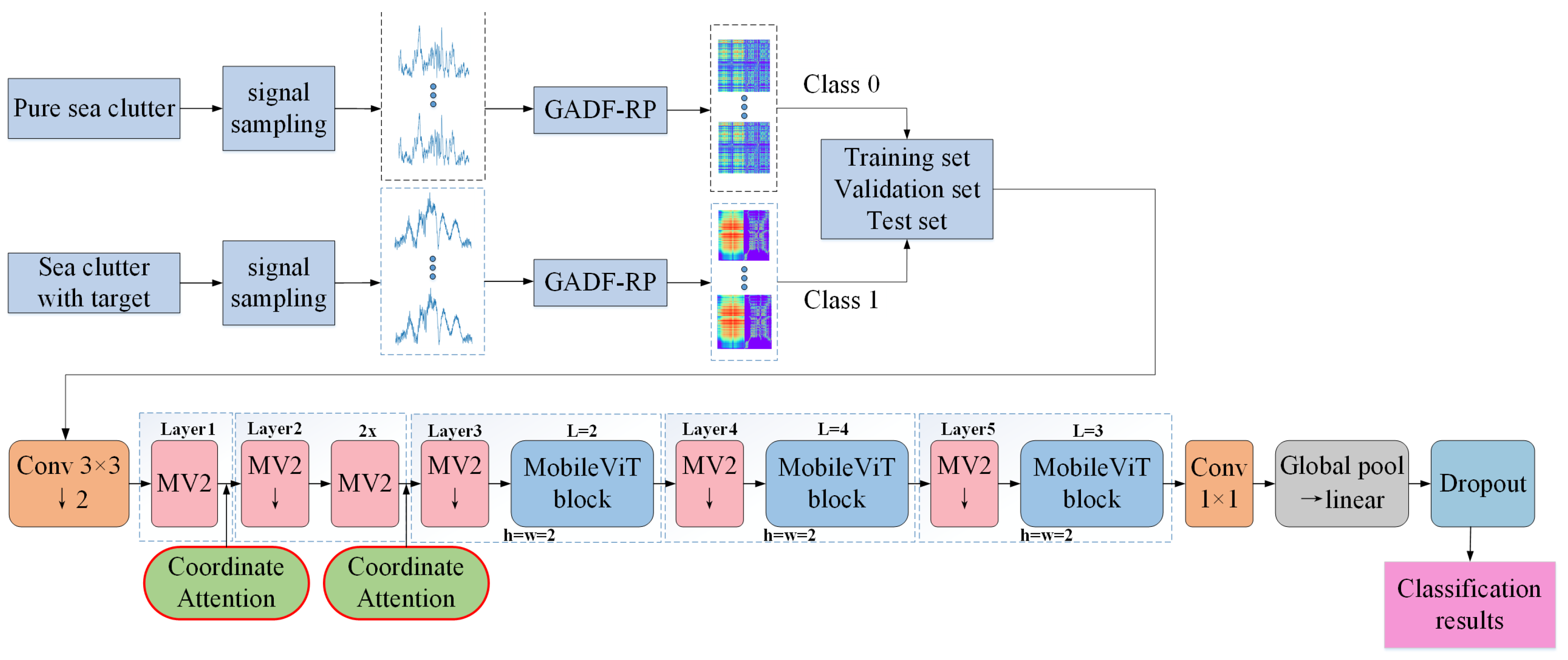
For this binary classification problem, the overall block diagram used in this study to achieve the intelligent classification of clutter and small targets is shown in Figure 3. First, sampling processing was carried out on the pure sea clutter signals and small-target signals. The length of the sampling sequence was set to 1024, and the sliding window size was set to 100. After sampling, the sequences are transformed into 2D dual-feature images via the GADF-RP method. Subsequently, the images corresponding to pure sea clutter signals were labeled with “0”, and those corresponding to small-target signals were labeled with “1”. The labeled images were then divided into a training set, a validation set, and a test set in a certain proportion. Finally, these datasets were input into the improved MobileViT model. The training set and validation set were used for model training and tuning, while the test set was used for the final performance evaluation. Eventually, the model outputs the classification results of the test set, achieving the intelligent classification of pure sea clutter and target signals.

3.1. MobileViT Network

Accurate information extraction is crucial in a sea surface small-target detection task. Due to the size of their convolutional kernels, traditional CNNs have a limited capacity to expand their receptive fields. The addition of layers to the network is likely to raise issues such as gradient explosions. ViTs [10] mark the beginning of a new milestone phase in image processing. It captures the global features of images through the global attention mechanism. 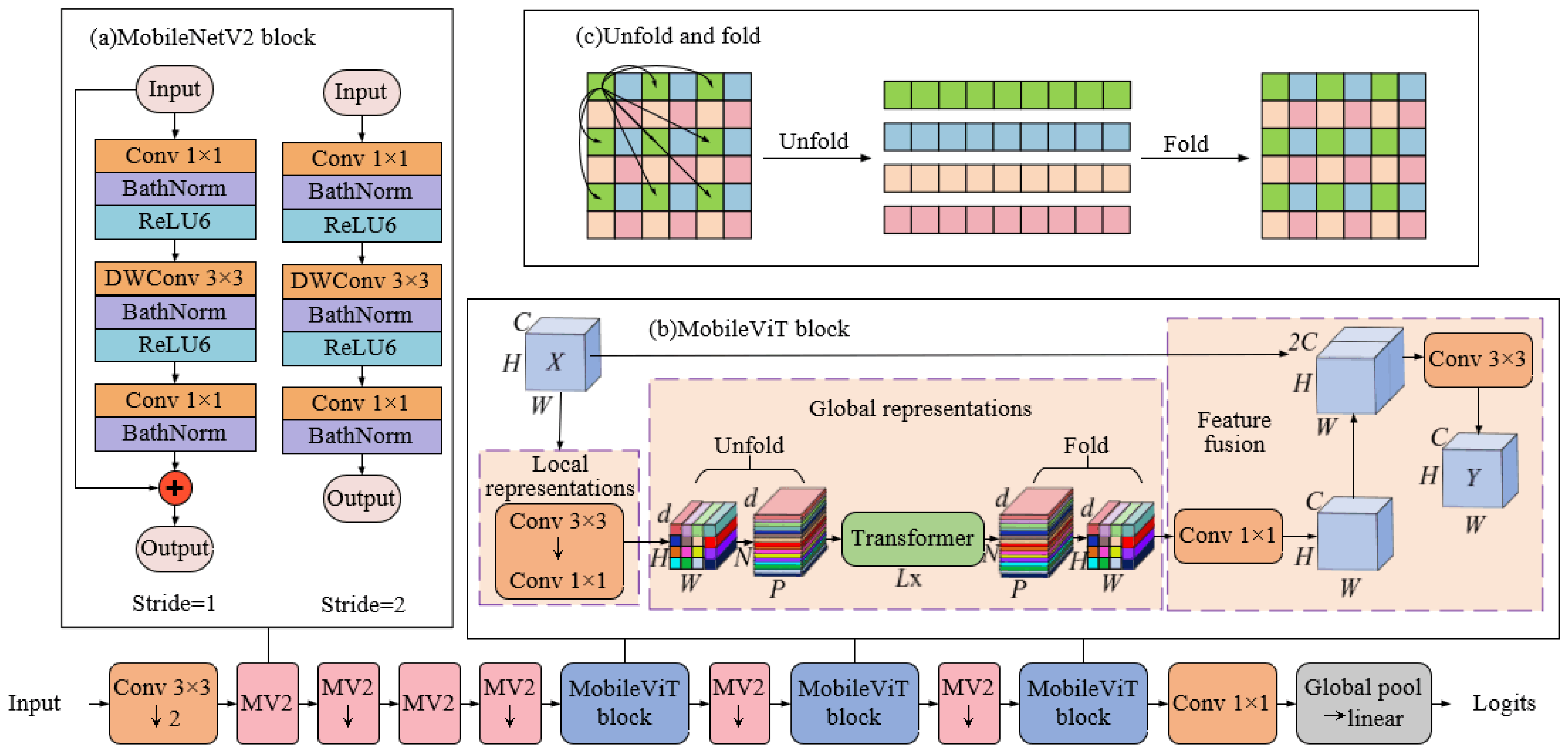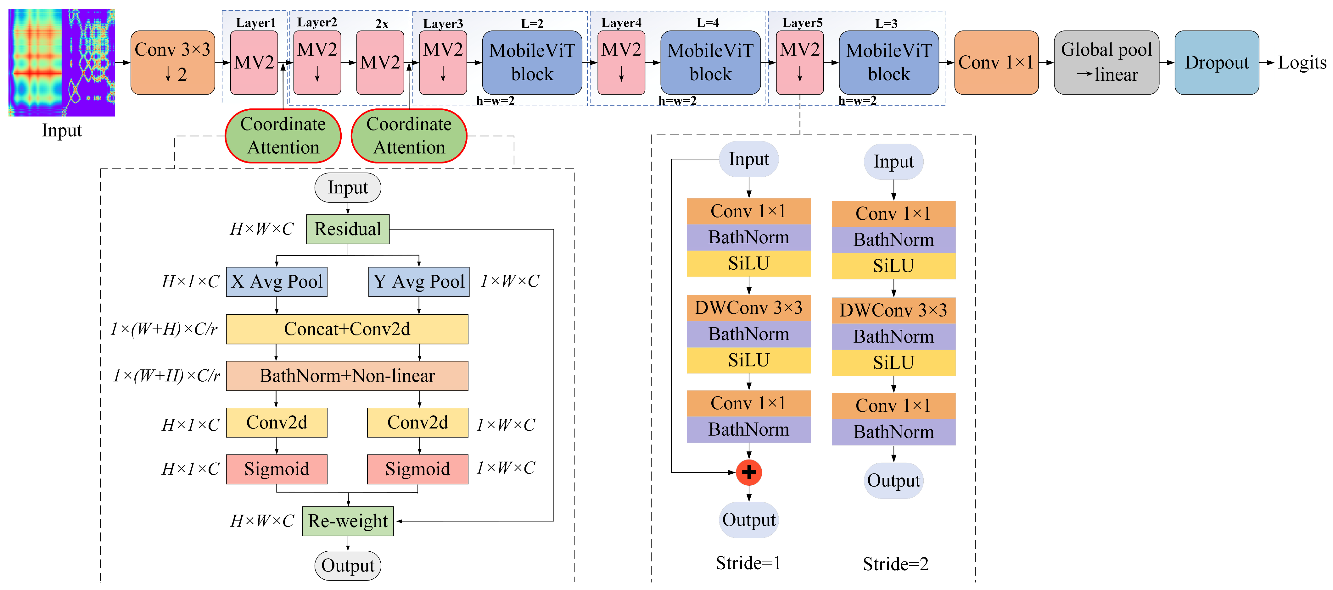Based on this, the MobileViT model [14] combines the local feature-capturing ability of CNNs and the global perception advantage of ViTs. It is a lightweight hybrid network structure aiming to improve the accuracy of small-target detection. The MobileViT model mainly consists of two core modules: the MobileNetV2 (MV2) module and the MobileViT module. The MobileViT module is further divided into three sub-modules: local representation, global representation, and feature fusion, which undertake different functions and enhance the model’s sensitivity to small targets in the detection task. The overall structure of MobileViT is shown in Figure 4.

(1)

MobileNetV2 module: The key to this module lies in its use of a depth-separable convolution and inverted residual structure, reducing the parameter number and computation amount, to speed up the model training and inference. The residual structure dimensionalizes the features and then upgrades them. In contrast, the inverted residual structure starts with a $1\times 1$ pointwise convolution to raise the features. It then utilizes a $3\times 3$ depth-separable convolution to extract features from each input channel separately. Finally, it further lowers the feature sizes with another $1\times 1$ pointwise convolution. Importantly, in the inversed residual structure, the activation function is usually ReLU6. The final pointwise convolutional layer employs a linear activation function to avoid low-dimensional information loss. Specifically, residual connections are introduced in the MV2 module only when the stride is 1. Series connections are used instead when the stride is 2.

(2)

MobileViT module: The design of this module aims to combine the advantages of local and global features to enhance the model’s perception ability for small targets in complex scenes. Through three sub-modules, namely local representation, global representation, and feature fusion [30,31], it optimizes the feature extraction process and strengthens the sensitivity to small targets.

The local representation module extracts the local features of the image through convolutional layers. For a feature image X of size $H\times W\times C$, the local features of the image are first extracted by a $3\times 3$ convolutional layer. Subsequently, the number of channels is adjusted to $d(d>C)$ by a $1\times 1$ convolutional layer, resulting in an adjusted feature image of size $H\times W\times d$. This process emphasizes the local information at each position in the feature image, which is crucial for the detection of small sea surface targets. Since the targets on the sea surface are often small and difficult to distinguish, local features enable the model to focus on the detailed features around the targets, enhancing the model’s sensitivity to small targets; in the global representation module, the feature image is divided into N image blocks of size $h\times w$, and there is no overlapping between blocks. It thus forms a sequence of image patches with a size of $P\times N\times d$ ($P=h\times w$). These patches are then input into the Transformer module to achieve a global feature encoding. After the encoding process, the patches are re-folded to resume their original dimensions. As shown in Figure 4c, this operation allows each image patch to perform attention computation exclusively with patches of the same color. In contrast, in ViT, all patches are engaged in attention computation, which significantly increases the overall computational burden. Global representation can assist the model in identifying and differentiating targets from clutter in complex backgrounds, thereby improving the detection accuracy of small targets; subsequently, a $1\times 1$ convolutional layer is employed in the feature fusion module to reduce the number of channels to C. This is then spliced with the original input feature images. Finally, the features are fused by a $3\times 3$ convolutional layer to obtain the output Y. The feature fusion module enables the model to further enhance the feature representation of the target area while retaining local and global information, thus improving the detection accuracy of small targets.

It should be noted that for the feature image X, in order to ensure the stability and efficiency of the network, it is necessary to crop the input images to a unified size during the data pre-processing stage. Unifying the input size can effectively avoid problems caused by inconsistent sizes during batch processing. In addition, cropping not only ensures the consistency of the model input but also effectively reduces the consumption of computational resources.

Through the close integration of local characterization, global characterization, and feature fusion, the feature extraction process is optimized, and the sensitivity to small targets is enhanced, enabling the MobileViT model to efficiently capture the features of small targets in sea clutter. Local characterization helps the model focus on the details of small targets, strengthening the feature expression in the target area. Global characterization, on the other hand, captures long-range dependencies through the global perception mechanism of the Transformer, improving the model’s global understanding of small targets. The feature fusion module further enhances the model’s detection ability by integrating local and global features. Especially in complex backgrounds, the recognition and discrimination of small targets are significantly strengthened.

3.2. Coordinate Attention Mechanism

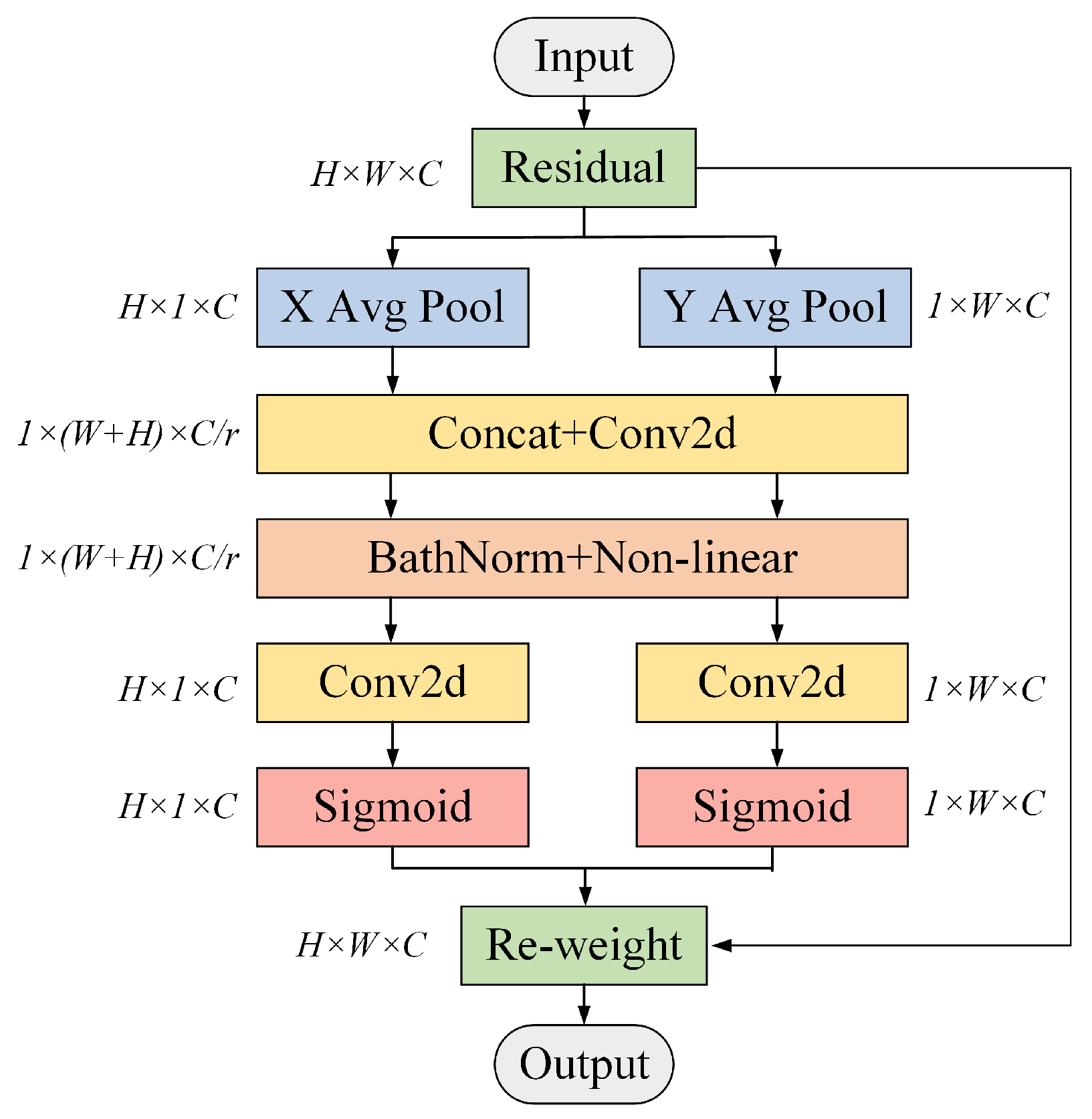
The coordinate attention (CA) mechanism simultaneously captures both channel- and direction-related spatial position information from the feature images. It is characterized by muscular flexibility and low computational complexity. Its introduction greatly enhances the model’s accuracy and its attention to key feature information. In this study, the CA mechanism is added to the MobileViT model, and the CA structure is shown in Figure 5 [32].

For the feature image x with an input size $H\times W\times C$, two feature images with positional information are obtained by performing one-dimensional pooling operations along the X and Y directions, respectively. The encoding mode of the cth channel $z_c^h(h)$ with height h (h < H) and the cth channel $z_c^w(w)$ with width w (w < W) is then expressed as follows:

$$z_c^h(h)={\displaystyle \frac{1}{W}}{\displaystyle \sum _{0\le i<W}{x}_c}(h,i)$$

(11)

$$z_c^w(w)={\displaystyle \frac{1}{H}}{\displaystyle \sum _{0\le j<H}{x}_c}(j,w)$$

(12)

The first two feature images are fused together with the location information, and use a $1\times 1$ convolution to compress the channel dimension to $C/r$. Moreover, BathNorm and the nonlinear activation function are used to extract spatial information features. The obtained intermediate feature image f is as follows:

$$f=\delta (F_1([z^h,z^w]))$$

(13)

where $\delta$ is a nonlinear activation function, $F_1$ is a $1\times 1$ convolution, and $[ , ]$ is a splicing operation along the spatial dimension. $f\in R^{C/r\times (H+W)}$ denotes the encoding of spatial information in the horizontal and vertical directions, where r is the reduction rate.

Following that, $f$ is divided into two separate tensors, $f^h$ and $f^w$, where $f^h\in R^{C/r\times H}$, and $f^w\in R^{C/r\times W}$. The channel numbers of $f^h$ and $f^w$ are made consistent with the input x by two $1\times 1$ convolutional transforms, and the resulting attention weights are:

$$g^h=\sigma (F_h(f^h))$$

(14)

$$g^w=\sigma (F_w(f^w))$$

(15)

where $g^h$ is the horizontal attention weight of x, $g^w$ is the vertical attention weight of x, $\sigma$ is the Sigmoid activation function, and $F_h$ and $F_w$ are the horizontal and vertical convolution operations. The final output of the entire coordinate attention block is expressed as follows:

$$y_c(i,j)=x_c(i,j)\times g_c^h(i)\times g_c^w(j)$$

(16)

where $x_c(i,j)$ and $y_c(i,j)$ are the inputs and outputs of the CA module, respectively, and $g_c^h(i)$ and $g_c^w(j)$ denote the horizontal and vertical attention weights on channel c, respectively.

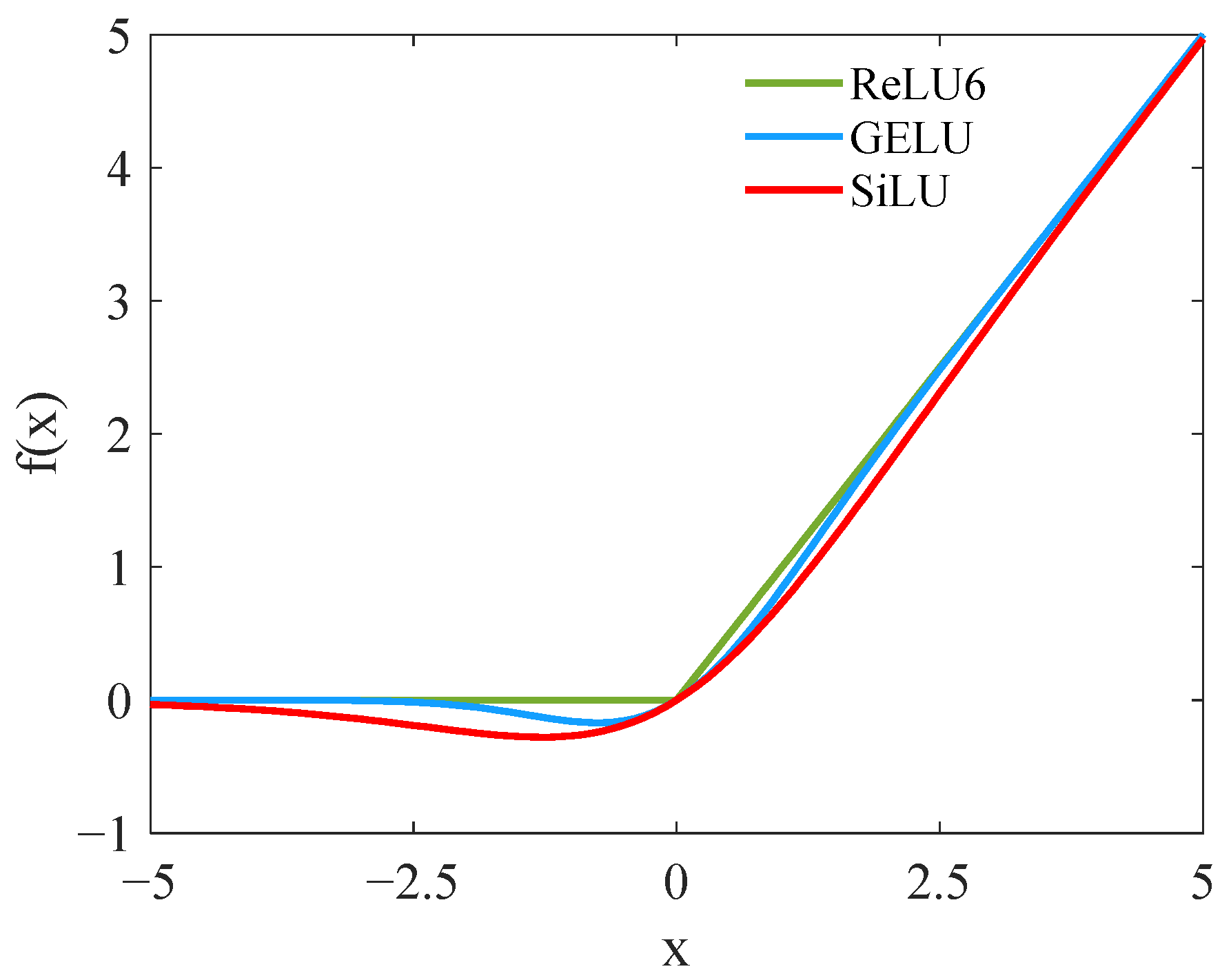
3.3. Selection of Activation Functions

The activation function in the MobileNetV2 module is typically ReLU6 [33], which is a variant of ReLU:

$$ReLU6(x)=\min (\max (0,x),6)$$

(17)

As is clear in Equation (17), ReLU6 controls the output range of neurons from 0 to 6, alleviating the gradient ReLU explosion and making the network training process more stable. However, ReLU6 still outputs 0 when the input is less than 0, which easily triggers neuron death and needs to be replaced with other activation functions.

Both GELU [34] and SiLU [35] are unbounded activation functions with functional expressions expressed in Equations (18) and (19), respectively:

$$GELU(x)=xP(X\le x) =x{\displaystyle \underset{-\infty }{\overset{x}{\int }}\frac{e^{-\frac{{(x-\mu )}^2}{2{\sigma }^2}}}{\sqrt{2\pi }\sigma }}dx\approx 0.5x(1+\tanh (\sqrt{{\displaystyle \frac{2}{\pi }}}(x+0.044715x^3))$$

(18)

$$SiLU(x)=x\cdot \sigma (x)$$

(19)

In Equation (18), $P(X\le x)$ is the probability function of the normal distribution, and $\mu$ and $\sigma$ are the mean and variance, respectively. In Equation (19), $\sigma (x)$ is the Sigmoid function.

Figure 6 shows images of the ReLU6, GELU, and SiLU activation functions. The ReLU6 function does not activate at all in the negative part. At the same time, GELU and SiLU allow negative values to have non-zero outputs, reducing the neuron death risk. In addition, both functions provide a smoother transition near x = 0, which helps improve the gradient flow and reduces the gradient vanishing. A comparison of SiLU to GELU reveals that SiLU behaves similarly to GELU around x = 0. However, the growth rate gradually exceeds GELU when x is greater than approximately 2, which has a more flexible correspondence than GELU does. Furthermore, the growth rate of SiLU is regulated by the input itself. This self-gating property provides a more effective activation for the network. Based on these findings and further experiments, SiLU is chosen as the activation function for the MobileNetV2 module.

3.4. Improved MobileViT Network Model

An enhanced MobileViT model is introduced in this study, as illustrated in Figure 7. The input sea clutter dual-feature image is first subjected to a $3\times 3$ convolutional layer for initial feature extraction and dimensionality reduction. This is followed by applying the MV2 module to Layers 1 and 2. The downward arrow with MV2 indicates Stride = 2, and the activation function ReLU6 is changed to the SiLU function with self-gating properties. CA is incorporated after Layers 1 and 2, which helps maintain the accurate position information while capturing long-distance dependencies in both the vertical and horizontal dimensions. This enhances the MobileViT basic model’s capacity to extract key information, thereby ensuring an improved detection accuracy. Subsequently, following the processes of down sampling and pooling, the extraction of features is conducted in multiple MV2 and MobileViT blocks from Layer 3 to Layer 5. Features are then aggregated after the network via a global pooling layer. Classification results, regardless of the target’s presence or absence, are obtained through a fully connected layer. To effectively mitigate overfitting, a Dropout layer is added after the fully connected layer to enhance the model’s generalization capabilities.

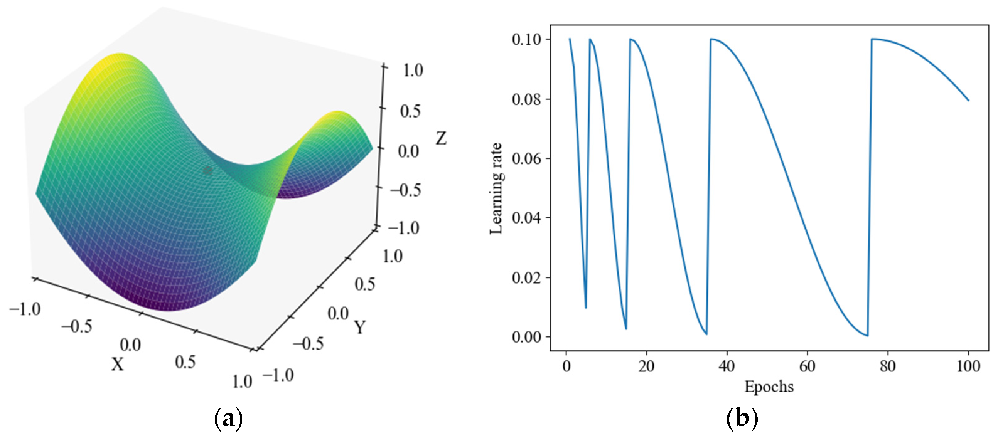
3.5. Cosine Annealing Algorithm

Training deep learning models is difficult because the learning process tends to fall into the saddle surface, as shown in Figure 8a. As a quadratic surface, the saddle surface has the property of being a maximum in one direction and a minimum in the other. In the region of the saddle surface, the first-order derivative of the loss function for the model parameters is 0, and the second-order derivative has both positive and negative values. A gradient of 0 thus leads to the stagnation of the parameter updates. In addition, the presence of saddle surfaces increases the risk of the model falling into local optimum solutions.

The cosine annealing algorithm [36,37] is chosen to automatically adjust the learning rate (LR), as shown in Figure 8b. During the training process, the LR does not simply decrease linearly or remain constant. Instead, it gradually decreases following an approximate periodic pattern. When decreasing to a minimal gradient, the LR immediately increases to the initial value, preventing the model from getting stuck in saddle points. This helps the model to converge better and increases its stability.

4. Experiments and Performance Analyses

Using real measured sea clutter data, this section demonstrates the validity of the proposed method through an experimental validation. The data are publicly available on the IPIX radar database website, provided by McMaster University in Canada [38]. Researchers at McMaster University collected the test data in Dartmouth, including various sea conditions, radar pulse frequencies, and polarization modes. The radar operates in the X-band, transmitting at a frequency of 9.39 GHz. Researchers gathered 14 sets of data for different sea conditions. Each set had 14 distance gates, with each gate containing 131,072 pulses. Four polarization modes were obtained according to their transmitting and receiving modes: HH, HV, VH, and VV.

Table 1. Information on IPIX radar data.

Dataset Name	Wind Speed (km/h)	Wave Height (m)	Angle (°)	Primary Target Unit	Sub-Target Unit
#17	9	2.2	9	9	8, 10, 11
#26	9	1.1	97	7	6, 8
#30	19	0.9	98	7	6, 8
#31	19	0.9	98	7	6, 8
#40	9	1.0	88	7	6, 8
#54	20	0.7	8	8	7, 9, 10
#280	10	1.6	180	8	7, 9, 10
#310	33	0.9	30	7	6, 8, 9
#311	33	0.9	40	7	6, 8, 9
#320	28	0.9	40	7	6, 8, 9

shows the information of 10 data groups used in their experiment. Among these, data group #17 corresponds to the highest wave height and represents high sea state conditions, while data group #280 represents medium sea state conditions. The remaining groups pertain to low sea state conditions [39].

To present the sea clutter data more intuitively, 300 sample points were selected from four sea conditions: #17, #26, #31, #54, #280, and #311. These data were used to create violin plots, as shown in Figure 9. The horizontal coordinates of these plots are marked with “-” and “+” to indicate the presence and absence of targets, respectively. The preliminary distribution of sample points reveals that the sea clutter wave amplitude of the target-free distance gates is small and relatively concentrated. In contrast, that of the targeted distance gates is relatively dispersed, with a small number of large values.

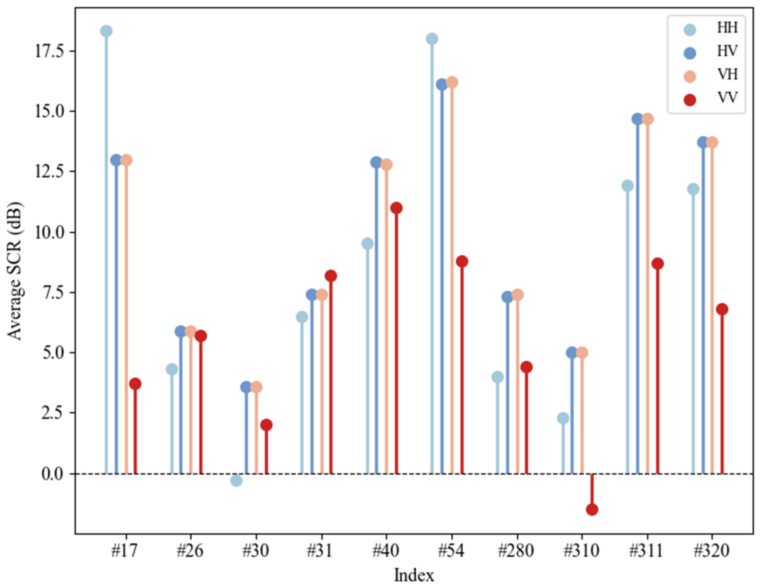
The average signal-to-clutter ratio (ASCR) is a pivotal metric for evaluating the data quality, as is illustrated in Figure 10. This figure presents the ASCR of the 10 data groups under the four polarization modes [40]. An observation of Figure 10 reveals that the signal-to-clutter ratio (SCR) under the HV and VH polarization modes is higher than that under the VV and HH polarization modes. Notably, the SCR values for data groups #26, #30, #280, and #310 are consistently low across all polarization modes. A relatively lower SCR indicates that the quality of the converted feature images for these four data groups in subsequent experiments is compromised, resulting in increased detection difficulties for the model.

4.1. Decision Threshold Adjustment Under a Constant False-Alarm Rate

In this binary classification, the pure sea clutter and target echo feature images were labeled as “0” and “1”, respectively. They were then input into the improved MobileViT model for training purposes. Once trained, the model recognized the feature images to be tested. The predicted output value $\rho$ from the model was then compared with the judgment threshold $\gamma$. When $\rho >\gamma$, it is judged as having a target, and when $\rho <\gamma$, it is judged as having no target, leading to the final classification result. However, the radar detection accuracy requires a high FAR of ${10}^{-3}$ to meet the detection standard among 1000 negative samples, of which 1 could be misclassified as a positive class. To achieve this, it is necessary to adjust the judgment threshold properly while keeping the FAR constant.

The probability that the input is predicted as a positive sample is $\xi$. Under a Monte Carlo experiment [41], n samples are used on the basis of the $H_0$ assumption with the improved MobileViT detection model, resulting in n statistics labeled as ${\xi }_1,{\xi }_2,\dots ,{\xi }_n$. For a given FAR of $P_{fa}$, the judgment threshold is therefore

$$\gamma ={\xi }_{[n\times P_{fa}]}$$

(20)

where [ ] denotes an integer to take. The process for adjusting the judgment threshold is illustrated in Figure 11. When the original threshold $\gamma =0.5$, the FAR is above ${10}^{-3}$, confirming the existence of many false alarms. To meet the detection standard, the judgment threshold is adjusted upward from the black dashed line to the red solid line position. This adjustment reduces the number of false alarms and meets the detection standard. The judgment threshold adjustment ensures that the model maintains a constant FAR.

4.2. Experiments on Dual-Feature Images of Sea Clutter

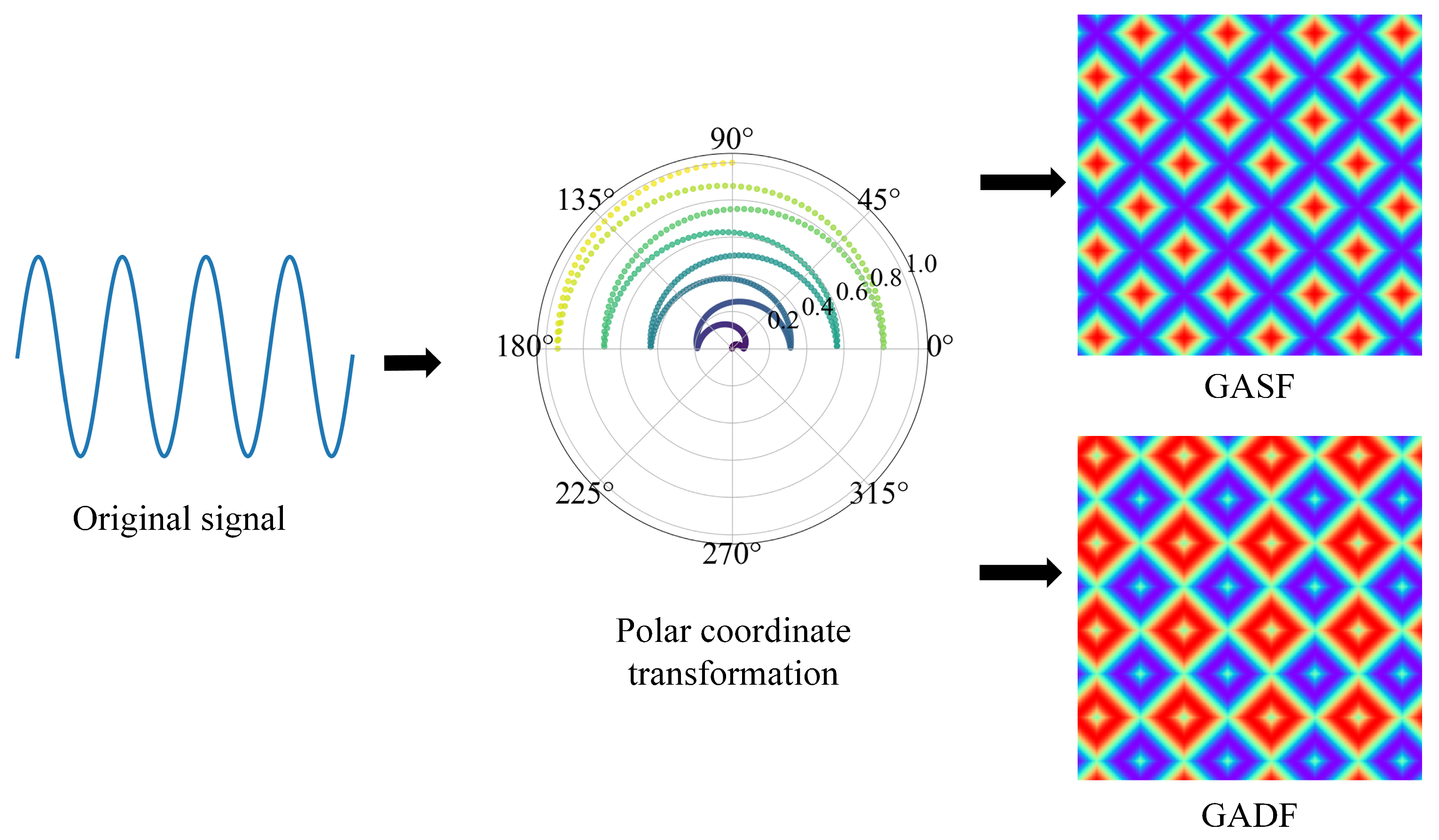
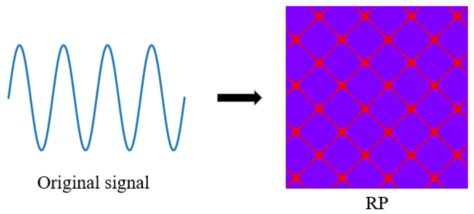
Section 2.1 presents the GAF model alongside two coding methods: GASF and GADF. It was found that the GADF method outperformed GASF in various perspectives [42]. Consequently, the GADF coding method was selected for a further investigation. From the original one-dimensional sea clutter time series, 1024 data points were sampled sequentially for both GADF and RP conversion, generating two corresponding $256\times 256$ two-dimensional feature images. Two feature maps were horizontally concatenated, and the size of the concatenated image was $512\times 256$. The size of the concatenated image was then readjusted to the size of the original single-feature map ($256\times 256$) through horizontal compression. This approach retains the key information from both coding methods, providing useful features for later modeling and detection. 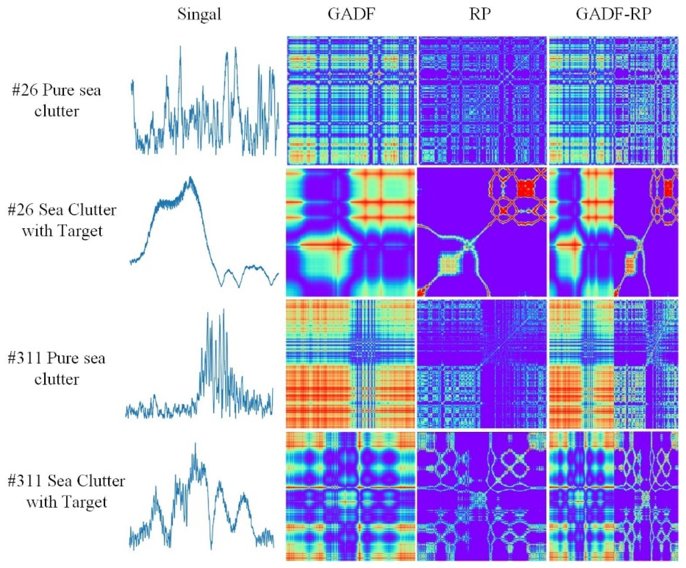As illustrated in Figure 12, the conversion flowchart consists of four rows.

Rows 1 and 2 present the time-series signal transformation diagrams for target-free (pure sea clutter) and targeted scenarios in sea state #26. In a very similar manner, sea state #311 is shown in rows 3 and 4. Using the time-series signal images alone, it is hard to distinguish the absence or presence of a target. The difference between the two-dimensional images after the conversion becomes much more apparent. The images of target-free distance gates present a certain degree of regularity and grid-like structure. In contrast, the images of targeted distance gates have multiple focus points and a more complex image that is visually distinguished.

By repeating the above operation and setting the sliding window to 100, it can generate 2600 spliced two-dimensional images for model training, validation, and testing for each dataset under various sea states.

4.3. Setting of Experimental Parameters

4.3.1. Selection of Batch Size

During the model construction process, the batch size determines the amount of data used for model training in each iteration. It directly impacts the model’s convergence speed, memory usage, and ultimate generalization ability. The sea state data under the 31st set of clutter HH polarization were selected. After converting these data into GADF-RP dual-feature images, we then divided them into a training set, a validation set, and a test set at a ratio of 70%, 15%, and 15%, respectively. Model training was implemented using Python environment 3.8, deep learning framework Pytorch 2.0.1, and Cuda version 11.8. In the training process, the cosine annealing algorithm was employed to automatically update the learning rate, with the learning rate range set from 0.000001 to 0.003.

Table 2. Training effects of the model with different batch sizes.

Batch Size	Epoch	Training Accuracy	Training Loss	Validation Accuracy	Validation Loss	Time (min)
2	50	0.928	0.186	0.913	0.203	52
2	100	0.998	0.007	0.977	0.050	104
2	150	0.998	0.003	0.992	0.035	157
4	50	0.952	0.132	0.949	0.158	42
4	100	0.996	0.012	0.982	0.045	86
4	150	0.997	0.008	0.989	0.029	129
8	50	0.950	0.116	0.941	0.172	36
8	100	0.992	0.018	0.985	0.042	72
8	150	0.999	0.004	0.995	0.019	108
16	50	0.953	0.119	0.936	0.154	32
16	100	0.997	0.014	0.995	0.023	65
16	150	0.999	0.007	0.997	0.012	97
32	50	0.960	0.107	0.921	0.199	33
32	100	0.988	0.031	0.967	0.103	65
32	150	0.998	0.010	0.979	0.053	98

(below) presents the influence of different batch sizes on the improved MobileViT model.

As can be observed from Table 2, under the same batch size, with every increment of 50 in the number of epochs, the accuracy of the training set and the validation set gradually increase and approached 1, while the loss values gradually decrease and approach 0. As the batch size increases, the running time for the model to iterate 150 times also decreases, ranging from a maximum of 152 min to a minimum of 97 min. However, a larger batch size does not always guarantee better performance. When the batch size is set to 32, the running time does not decrease; instead, it increases by one minute. Moreover, when the number of epochs reaches 150, the accuracy of the validation set is 0.979, indicating a decline in model performance, which is lower than the accuracies achieved when the batch size is 2, 4, 8, and 16. Therefore, considering both the running time and the accuracies of the training and validation sets, a batch size of 16 is deemed the most appropriate choice.

4.3.2. Influence of Attention Mechanisms

To verify the effectiveness of adding the CA mechanism after the first and second layers of MobileViT, three other attention mechanisms were selected for comparison: the Global Attention Module (GAM) [43], the Convolutional Block Attention Module (CBAM) [44], and the Squeeze-and-Excitation block (SE) [45]. These are inserted at the same positions in the model, and all parameters remain consistent except for the attention mechanisms. The experimental results are presented in

Table 3. Influence of different attention mechanisms on detection results.

Attention Mechanism	Batch Size	Epoch	Accuracy
GAM	16	150	0.9103
CBAM	16	150	0.9821
SE	16	150	0.9846
CA	16	150	0.9897

. The CA mechanism shows the best performance, while the GAM has a relatively lower accuracy.

4.3.3. Influence of Activation Functions

Based on the theoretical introduction of activation functions in Section 3.3, the ReLU6, GELU, and SiLU activation functions are selected for experimental comparison.

Table 4. Influence of different activation functions on detection results.

Activation Function	Batch Size	Epoch	Accuracy
ReLU6	16	150	0.9641
GELU	16	150	0.9641
SiLU	16	150	0.9897

explores the influence of these three activation functions in the MobileNetV2 module on the detection results. Under the same parameter conditions, the SiLU activation function performs optimally in the MobileNetV2 module, with the model’s detection accuracy reaching 0.9897. This shows a significant improvement compared to the accuracies of 0.9641 achieved by ReLU6 and GELU, indicating that the SiLU activation function is more suitable for enhancing the model’s detection performance.

4.4. Comparison of Feature Image Effects Across Different Conversion Methods

At a constant FAR of ${10}^{-3}$, GADF, RP, and GADF-RP splicing transformations were performed separately on high-sea-state data (#17, #280) and low-sea-state data (#26, #310) for both the HH and VV polarization modes. The improved MobileViT model then classified the transformed feature images, as illustrated in Figure 13. Under the same classification model, the detection results were optimal after applying the GADF-RP transformation across various datasets. However, an exception occurred here: the RP and GADF-RP feature images yielded identical detection results in the #280 dataset in the VV polarization mode. This is attributed to the superior image quality of the #280 dataset. The difference between the maximum detection probabilities of the same group data reached 7.4%. Overall, a single RP conversion demonstrates a greater effectiveness compared to a single GADF transformation. Combining the feature images of the two approaches, the improved MobileViT model extracts more compelling information, thus improving the detection performance.

4.5. Comparison of MobileViT Model Before and After the Improvement

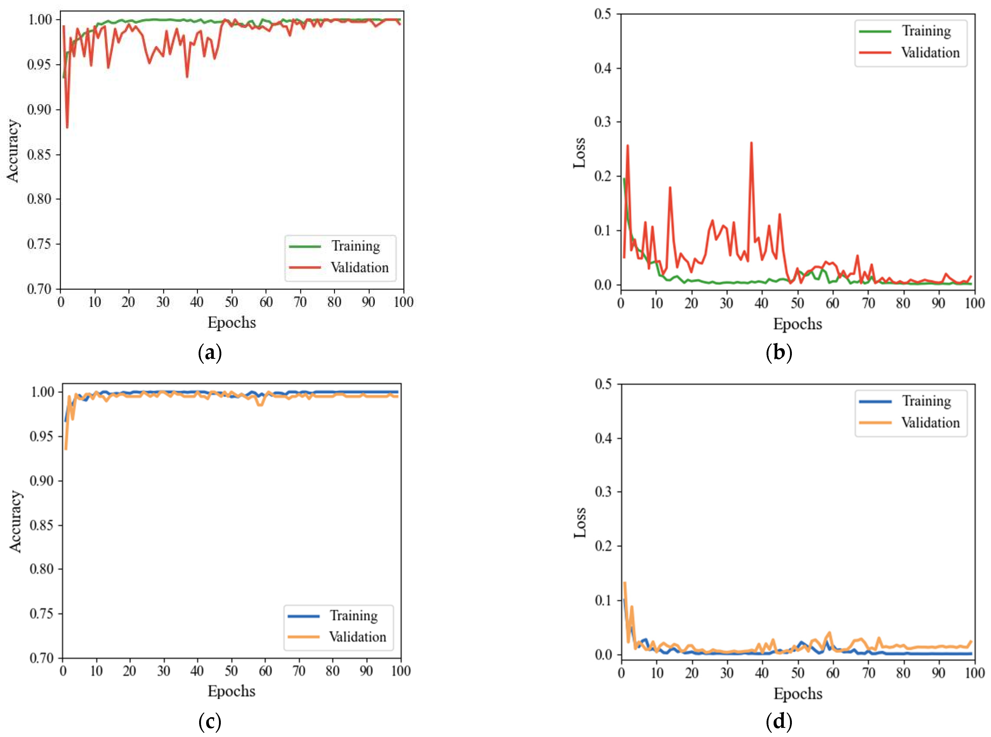
The images were trained with the unimproved and improved MobileViT models following the selection of the #54 dataset under HH polarization mode and their conversion into feature images by GADF-RP. The accuracies and loss values of the two models were then compared in the training and validation sets. As Figure 14 shows, when comparing Figure 14a with Figure 14b,c with Figure 14d, the accuracy and loss value curves of the former validation set fluctuate significantly and only slowly converge and stabilize after about 50 iterations. In contrast, the latter converges rapidly with a slight fluctuation, and the entire curve becomes more stable. The accuracy of the final MobileViT test set is 98.97%, and the accuracy of the improved MobileViT test set is 99.74%, respectively, thus confirming that the improved model facilitates the key feature extraction of sea clutter waves and enhances the training efficiency and general performance.

4.6. Comparison of Different Model Performances

The model performance was evaluated using six metrics, namely accuracy, precision, recall, F1-score, FAR, and missing alarm rate (MAR), on the test set of dual-feature images [46], as shown in Equations (21)–(26).

$$Accuracy={\displaystyle \frac{TP+TN}{TP+TN+FP+FN}}$$

(21)

$$Precision={\displaystyle \frac{TP}{TP+FP}}$$

(22)

$$Recall={\displaystyle \frac{TP}{TP+FN}}$$

(23)

$$F1={\displaystyle \frac{2\times Precision\times Recall}{Precision+Recall}}$$

(24)

$$FAR={\displaystyle \frac{FP}{FP+TN}}$$

(25)

$$MAR={\displaystyle \frac{FN}{FN+TP}}$$

(26)

These metrics can all be calculated from the confusion matrix of the results, as shown in

Table 5. Definition of the confusion matrix.

	Predicted Negative	Predicted Positive
Actual Negative	True Negative (TN)	False Positive (FP)
Actual Positive	False Negative (FN)	True Positive (TP)

. In the equations above, TP denotes that the targeted feature image is correctly predicted as targeted; TN denotes that the untargeted feature image is correctly predicted as untargeted; FP denotes that the wrongly untargeted feature image is predicted as targeted; and FN denotes that the targeted feature image is wrongly predicted as untargeted [47].

To verify the effectiveness of the improved MobileViT model and avoid the contingency of the experiments, three groups of sea state data, #17, #31, and #310, were selected under the HH polarization of sea clutter. Time-series signals were converted into GADF-RP dual-feature images that were divided into training, validation, and test sets, according to a split of 70%, 15%, and 15%, respectively. The experimental parameters were kept the same without setting the false-alarm rate. The improved MobileViT model was compared with CNN [8], ViT [10], ShuffleNetV2 [48], MobileNetV3 [49], Swin Transformer [50], ConvNeXt [51], and MobileViT [15]. After the test was completed, the performance of the model was evaluated based on the metrics of Equations (21)–(26), and the results are shown in

Table 6. Comparison of model performances under sea state data from group #17.

Model	Accuracy	Precision	Recall	F1-Measure	FAR	MAR
CNN	0.9385	0.9476	0.9282	0.9378	0.0513	0.0718
ViT	0.9410	0.9831	0.8974	0.9383	0.0154	0.1026
ShuffleNetV2	0.9744	0.9744	0.9744	0.9744	0.0256	0.0256
MobileNetV3	0.9769	0.9895	0.9641	0.9771	0.0103	0.0359
Swin Transformer	0.9795	0.9947	0.9641	0.9783	0.0051	0.0359
ConvNeXt	0.9026	0.9153	0.8872	0.9016	0.0821	0.1128
MobileViT	0.9769	0.9794	0.9744	0.9768	0.0205	0.0256
Improved MobileViT	0.9846	0.9900	0.9795	0.9847	0.0103	0.0205

,

Table 7. Comparison of model performances under sea state data from group #31.

Model	Accuracy	Precision	Recall	F1-Measure	FAR	MAR
CNN	0.9086	0.9133	0.9043	0.9088	0.0869	0.0957
ViT	0.9205	0.9362	0.9026	0.9191	0.0615	0.0974
ShuffleNetV2	0.9667	0.9789	0.9538	0.9662	0.0205	0.0462
MobileNetV3	0.9846	0.9846	0.9846	0.9846	0.0154	0.0154
Swin Transformer	0.9744	0.9695	0.9795	0.9745	0.0308	0.0205
ConvNeXt	0.8410	0.9359	0.7333	0.8225	0.0513	0.2667
MobileViT	0.9769	0.9697	0.9846	0.9771	0.0308	0.0154
Improved MobileViT	0.9897	0.9948	0.9846	0.9897	0.0051	0.0154

and

Table 8. Comparison of model performances under sea state data from group #310.

Model	Accuracy	Precision	Recall	F1-Measure	FAR	MAR
CNN	0.9487	0.9581	0.9385	0.9482	0.0410	0.0615
ViT	0.9615	0.9839	0.9385	0.9606	0.0154	0.0615
ShuffleNetV2	0.9846	0.9948	0.9744	0.9845	0.0051	0.0256
MobileNetV3	0.9795	0.9895	0.9692	0.9795	0.0103	0.0308
Swin Transformer	0.9872	1	0.9750	0.9873	0	0.0250
ConvNeXt	0.9026	0.9198	0.8821	0.9058	0.0769	0.1179
MobileViT	0.9821	0.9747	0.9897	0.9841	0.0256	0.0103
Improved MobileViT	0.9872	0.9897	0.9846	0.9871	0.0103	0.0154

. The data under the three sea state conditions in Table 6, Table 7 and Table 8 were averaged and sorted in descending order according to the accuracy. The sorted results are shown in

Table 9. Comparison of average model performances.

Sort	Model	Accuracy	Precision	Recall	F1-Measure	FAR	MAR
1	ConvNeXt	0.8821	0.9237	0.8342	0.8766	0.0701	0.1658
2	CNN	0.9319	0.9397	0.9237	0.9316	0.0597	0.0763
3	ViT	0.9410	0.9677	0.9128	0.9393	0.0308	0.0872
4	ShuffleNetV2	0.9752	0.9827	0.9675	0.9750	0.0171	0.0325
5	MobileViT	0.9786	0.9746	0.9829	0.9793	0.0256	0.0171
6	MobileNetV3	0.9803	0.9879	0.9726	0.9804	0.0120	0.0274
7	Swin-Transformer	0.9804	0.9881	0.9729	0.9800	0.0120	0.0271
8	Improved MobileViT	0.9872	0.9915	0.9829	0.9872	0.0086	0.0171

.

As illustrated in Table 9, the classical CNN model achieves an average accuracy rate of about 93%. However, with a relatively high FAR, it fails to meet the requirement of low FAR for radar detection. The average accuracy of the ViT model alone is slightly higher than that of the CNN, implying that a mere reliance on either local or global features does not yield the best detection performance. Combining the advantages of CNN and ViT, the lightweight MobileViT model has an average accuracy of 97.86% with a FAR of 2.56%. The improved MobileViT model has an average accuracy of 98.72% and a FAR of 0.86%. Compared to the original MobileViT model, this improved model boasts a 0.86% increase in average accuracy and an order of magnitude decrease in false-alarm rate. Conversely, the ConvNeXt model, despite its enhancement from the Swim Transformer structure, places a greater reliance on local image information in its classification task. As a result, it is more suitable for small datasets or low-resolution images, yielding a lower detection accuracy. This highlights the necessity for a model to possess a strong capability for global perception.

4.7. Full-Sample Experiment on the Dataset

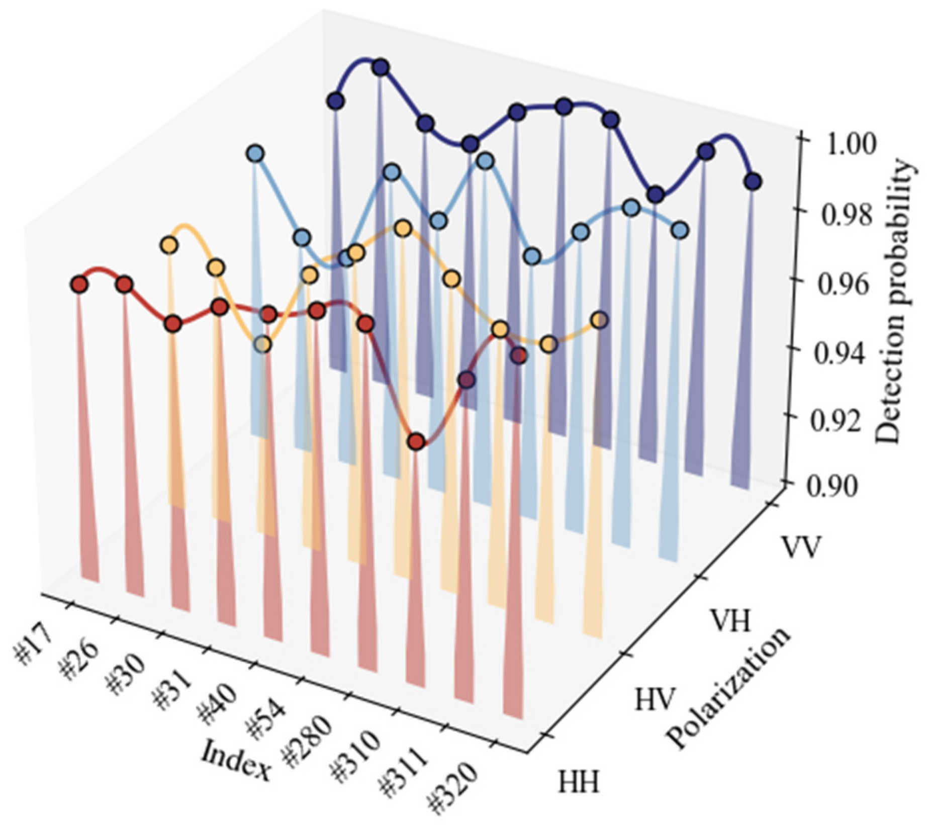
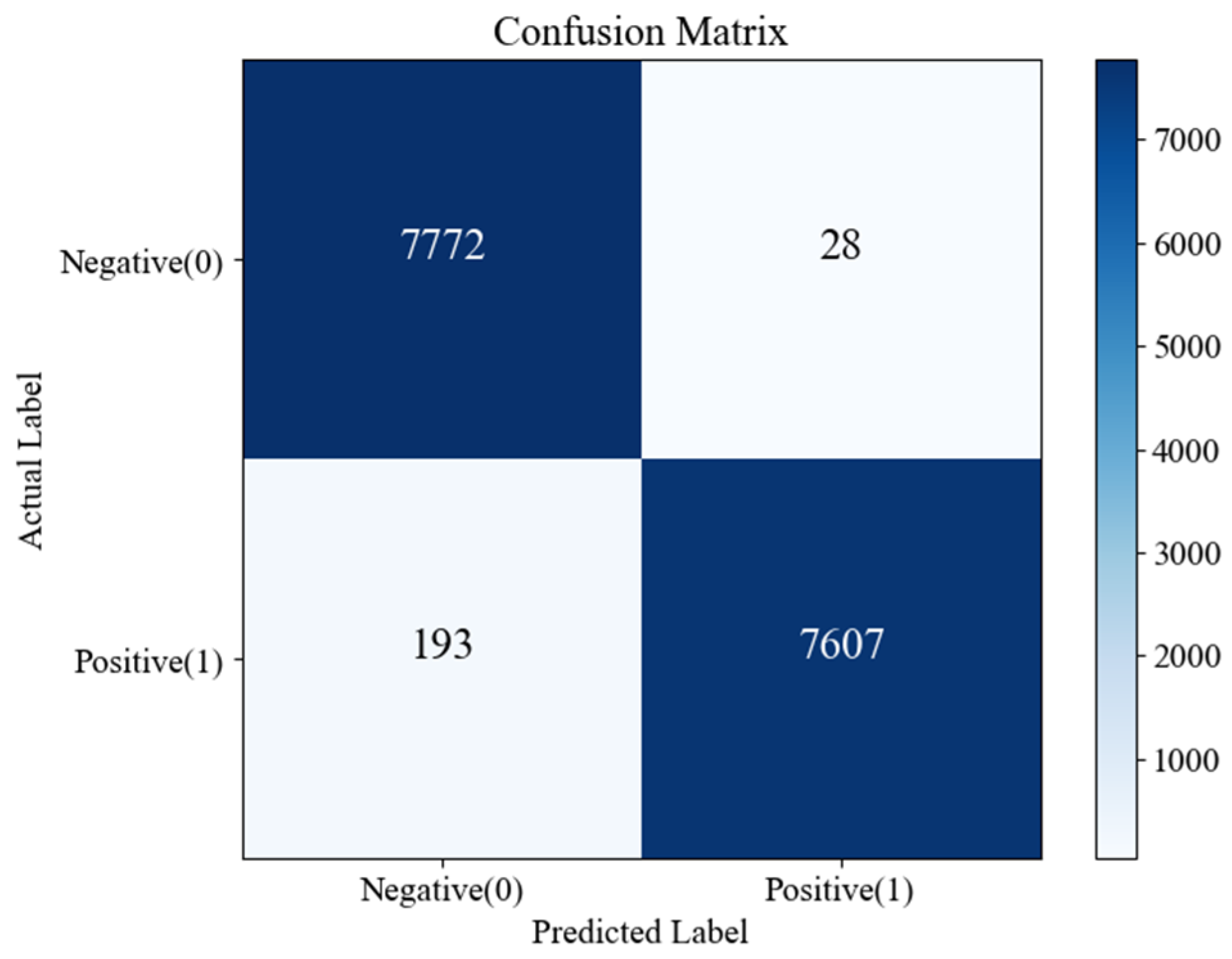
This study proposes a detection method based on dual-feature images and improved MobileViT. It was tested against all the data in Table 1, maintaining a constant FAR of ${10}^{-3}$. The results in Figure 15 demonstrate that the lowest and highest detection probabilities are 95.6% and 100%, respectively, under the four polarization modes of HH, HV, VH, and VV. To better analyze the overall detection effect of the proposed method, the total confusion matrix of the 10 sea situations is plotted in Figure 16. Among the test images, 28 are misclassified as having targets, while 193 are misclassified as having no targets, with an overall detection probability of 98.6%.

During the training process of the improved MobileViT detector, the detection probability achieves over 93% at approximately 25 iterations for data groups #26, #30, and #310, characterized by a lower signal clutter. Conversely, for data groups exhibiting a higher SCR, the detection probability reaches 100% at around 10 iterations. The improved MobileViT model demonstrates its accuracy, effectiveness, and swiftness classification task performance, even with images of unsatisfactory sea clutter quality. This is attributed to its combining local feature extraction from CNN, global perception via ViT, and spatial location capturing through the CA mechanism.

4.8. Discussion and Method Comparison

4.8.1. Comparison of Methods

Three other novel methods for small surface target detection will now be compared, typically using images, machine learning, and deep learning, respectively: graph connectivity density (GCD) [5], the GA-XGBoost detector based on FAST four-feature extraction [52], and the Bi-LSTM detector based on 3D sequence features [53].

Table 10. Comparison of different methods for detecting small floating targets on the sea surface.

References	Dataset	Methods	Average Accuracy
Yao et al. [5]	IPIX	GCD detector based on construction of graphs	0.373
Zhao et al. [52]	IPIX	GA-XGBoost detector based on FAST four-feature extraction	0.692
Wan et al. [53]	IPIX	Bi-LSTM detector based on 3D sequence features	0.955
Our	IPIX	Improved MobileViT based on dual-feature images	0.986

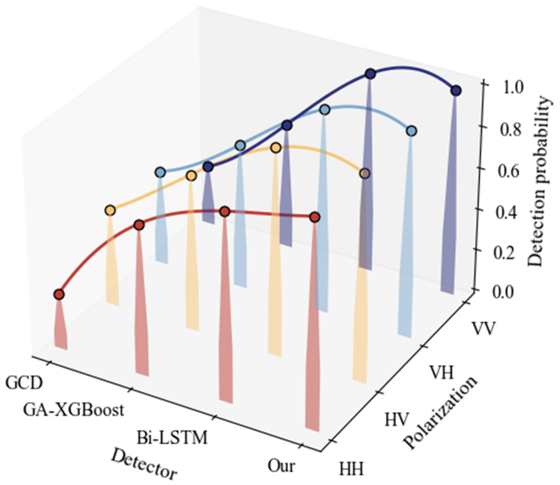
presents their detection methods and the average detection probabilities on the IPIX dataset. Figure 17 shows the detection results under the four polarization modes (HH, HV, VH, and VV) on the IPIX dataset. The observations of the data distributions (Figure 17) reveal that the two deep learning detectors, Bi-LSTM and the proposed improved MobileViT, are significantly better than the previous two. The average detection probability for the Bi-LSTM model is 95.5% across four polarization modes, and that of the proposed improved MobileViT is 98.6%. In comparison, the average detection probability of GCD and GA-XGBoost is merely 37.3% and 69.2%, respectively. These results confirm that the best detection effect is realized through the improved MobileViT model.

In summary, in the experimental part of this section, the effectiveness of the proposed detection method is validated in four different aspects using IPIX sea surface clutter data. The comparison results are summarized in

Table 11. Summary of comparison results in four aspects.

Comparison Methods	Objects Compared	Results
Effects of feature image transformation	GADF, RP, and GADF-RP	The detection probability of GADF-RP with dual-feature images is higher than that with a single-feature image.
Before and after the model improvement	MobileViT and improved MobileViT models	The improved MobileViT model exhibits strong generalization ability and higher detection accuracy.
Different classifiers	CNN, ViT, ShuffleNetV2, MobileNetV3, Swin Transformer, and ConvNeXt	The improved MobileViT model achieves the highest accuracy and the lowest FAR.
Relatively novel detection methods in recent years	GCD, GA-XGBoost, and Bi-LSTM	The average detection rate of the improved MobileViT model is 98.6%, outperforming the other three at 37.3%, 69.2%, and 95.5%, respectively.

.

The results summarized in Table 11 demonstrate a superior detection performance in the following aspects:

• The splicing method transforms a single-feature image into one with a double feature, resulting in a converted feature image of the time-series signal. It concurrently encompasses the information in the two encoding modes. This approach provides some substantial advantages in terms of information completeness, feature diversity, and the subsequent detection performance, compared with the single conversion method.
• A deep learning approach is employed and incorporated with an attention mechanism. Traditional detection methods rely on statistical theories, fractal properties, chaotic properties, various feature extraction techniques, and standard machine learning methods. Compared to these methods, the detection probability of the deep learning is improved by 20% to 50%. In addition, the detection results in Table 9 illustrate that a suitable deep learning classification model needs to be selected and combined with the attention mechanism to further improve the classification accuracy.
• The detection results are not affected by the quality of the original data. A low signal-to-clutter ratio of the original IPIX part in the dataset makes it difficult to identify the target. This affects the model classification accuracy. Other classical detection methods have much lower detection probabilities than those of HV and VH under HH and VV polarization modes. Among all current sea clutter detection methods, the Bi-LSTM detector demonstrates the highest detection probability, utilizing three-dimensional sequence features. The average detection probability under HV, VH, and VV is above 96%. In comparison, the detection probability under HH is 89.5%, also affected by the low signal-to-clutter ratio of the data. The average detection probability of the four polarization modes of the proposed method is above 98%, with balanced experimental results.

4.8.2. Future Outlook and Directions for Improvement

• Optimization of model efficiency: Although the detection results of the proposed method are not affected by data quality, when dealing with low signal-to-noise-ratio data, the model requires a long training time to converge. In practical application scenarios, such as offshore mobile monitoring platforms, the computing resources are often limited. Therefore, it is necessary to simplify the model structure while maintaining a high detection rate, so as to save resources and accelerate the detection process.
• Improvement of denoising processing: Affected by the noise generated by the radar itself during the detection process and the harsh sea surface environment, some high -frequency clutter signals may be misjudged as small-target signals during the detection process. For these outliers, denoising techniques can be used to pre-process the original signals to further improve the detection accuracy. Specifically, for the nonlinear and non-stationary characteristics of sea clutter signals, the empirical mode decomposition and its improved methods can be used to decompose the sea clutter signals into multiple intrinsic mode functions, so as to distinguish the noise and target signal components. In addition, wavelet transform and multi-threshold processing methods can be used to effectively separate the noise and target signals. In the future, deep learning-driven noise suppression methods can be considered, such as embedding a learnable denoising layer in the target detection network to achieve efficient denoising and further improve the detection accuracy.
• Enhancement of temporal quantification: When processing sea clutter signals, the method proposed in this study has room for improvement in quantifying the uncertainty of temporal dependencies in the input and output. Novel automatic prediction deep learning methods typically utilize advanced time-series analysis techniques, such as long short-term memory networks (LSTMs) and their variants, which can better capture long-term dependencies in time series. Future research can explore the combination of more advanced time-series modeling methods with existing image processing and deep learning techniques to more accurately quantify the uncertainty of temporal dependencies, thereby further enhancing the stability and accuracy of small-target detection on the sea surface. For example, an attempt can be made to fuse the time-series model based on the attention mechanism with the MobileViT network. This enables the model, when processing sea clutter signals, to not only effectively extract spatial features but also precisely grasp the uncertainty of temporal dependencies, thus achieving more reliable small-target detection in the complex and variable marine environment.

5. Conclusions

Due to the complex nonlinear and non-stationary characteristics of sea clutter, the detection of small targets in the sea clutter background has always been a major challenge in the field of maritime surveillance, and it is of great significance for enhancing maritime safety and target recognition capabilities. To address this issue, this study proposes an intelligent detection method for small sea surface targets that combines images and deep learning. By using the GADF-RP method to convert 1D sea clutter time-series signals into 2D feature images, and designing an improved MobileViT network as a classifier, a new detection scheme for small sea surface target detection is constructed. The key technological innovations include enhancing the discriminability of small sea surface targets through a dual-feature mechanism, introducing a CA mechanism to enhance feature discrimination ability, replacing the ReLU6 activation function in the MV2 module with the SiLU activation function to improve nonlinear expression ability, and adopting the cosine annealing algorithm to achieve dynamic learning rate optimization.

Experimental verification was carried out on the IPIX dataset. The experimental results from multiple aspects indicate that (1) the performance of the GADF-RP dual-feature images is superior to that of the GADF or RP single-feature images; (2) compared with the original MobileViT model, the improved one has a faster convergence speed, more stable performance, and higher detection accuracy; (3) compared with other neural network models, it has higher accuracy and a lower false-alarm rate; and (4) compared with other current advanced small sea surface target detection methods, the detection probabilities under the four polarization modes are balanced, all above 98%, and the average detection probability is as high as 98.6%. These results confirm the feasibility of the technical route of fusing deep learning technology after converting time-series signals into images, marking a paradigm shift from traditional sea clutter signal processing methods to a data-driven deep learning framework.

This method demonstrates potential application value in coastal surveillance scenarios, capable of significantly enhancing the recognition reliability of small sea surface buoy targets. Through this joint optimization method of radar data feature extraction and classification, it provides a technical reference for constructing a lightweight intelligent radar detection system.

Future research can optimize small sea surface target detection in multiple aspects: (1) Optimizing model efficiency. In resource-constrained scenarios such as offshore mobile monitoring platforms, the model structure can be simplified to accelerate the detection process. (2) Improving denoising processing. Try to adopt deep learning-driven noise suppression methods to further enhance detection accuracy. (3) Enhancing time quantification. Explore the combination of advanced time-series modeling methods with existing technologies, such as fusing the attention-based time-series model with the MobileViT network, to improve the stability and accuracy of detection.