A Novel Autonomous Marine Profile Elements Monitoring and Sample Collection System

Abstract

This study develops an autonomous ocean observation system designed for continuous, multidimensional marine parameter monitoring. The system integrates sensor-based monitoring and sample collection capabilities, utilizing tidal energy to facilitate vertical movement within the water column (0–50 m). The system combines tidal energy utilization with a buoyancy regulation unit, significantly reducing reliance on conventional battery power while maintaining the system’s flexibility in deep control, demonstrating superior energy efficiency compared to traditional platforms. The combination of sensor monitoring and sample acquisition enables real-time acquisition of oceanographic parameters (e.g., temperature, salinity, chlorophyll) and on-demand water sample collection for high-precision laboratory analysis. Laboratory and sea trials validated its ability to perform reciprocating vertical motion, autonomous buoyancy regulation, and leak-free sample collection, confirming feasibility for long-term coastal ecosystem monitoring. This study highlights the potential of autonomous systems for sustainable ocean observation and environmental monitoring.

1. Introduction

In recent years, the degradation of coastal ecosystems has emerged as a significant concern among scientists, prompting extensive research on how to improve the marine environment [1,2]. To effectively address and mitigate the impacts of this degradation while promoting human understanding and utilization of the ocean, it is imperative to conduct long-term, continuous, and multidimensional monitoring in targeted areas. Such monitoring should encompass various oceanic environmental parameters, including ocean currents, chlorophyll concentrations, nutrient levels, temperature variations, and salinity. Through these comprehensive measurements, we can not only gain a deeper understanding of the dynamic processes driving ecosystem changes and develop informed strategies for conservation and restoration but also enhance human knowledge of marine resources and their sustainable use for economic, scientific, and societal benefits.

Traditional methods for measuring oceanic parameters—such as on-site assessments conducted via ships or moored instruments—are evidently inadequate for achieving long-term continuous multidimensional monitoring of marine areas. However, advancements in marine equipment technology are facilitating a transition from discrete single-point measurements towards continuous profiling throughout the water column. This shift represents a move away from ship-based observations toward autonomous marine observation systems [3].

Among these systems, the Argo float is currently the most recognized and widely deployed profiling platform, providing continuous observational data on oceanic temperature, salinity, and pressure parameters from the sea surface to a depth of 2000 m [4]. Argo floats utilize batteries to power a piston pump that regulates the movement of oil between an internal bladder and an external rubber bag. This mechanism alters the float’s buoyancy and facilitates adjustments in its depth. As of September 2018, Argo had recorded approximately 2,000,000 ocean profiles with around 4000 operational Argo floats [5].

The McLane Moored Profiler (MMP) represents another significant platform for profiling measurements. It is primarily equipped with a CTD (Conductivity, Temperature, Depth) sensor and an acoustic current meter, enabling continuous observations of oceanic temperature, salinity, depth, and currents within a range extending up to 6000 m [6]. Another type of profiling platform is the Autonomous Moored Profiler (AMP), which is specifically designed to monitor water quality at designated geographical locations with depths less than 50 m [7].

Given the scarcity of electrical resources in marine environments, there is growing emphasis on exploring alternative energy sources to power marine observation systems. To enhance the longevity of these systems and reduce energy consumption, many institutions are now focusing on developing technologies that utilize wave energy, ocean thermal gradient energy, ocean current energy, and gravitational potential energy as primary power sources. This shift not only addresses the critical challenge of limited electrical resources but also significantly extends the operational lifetimes of marine observation systems.

The potential energy-driven reciprocating ocean profiler (PedROP) prototype developed by Ocean University of China features a CTD sensor for measuring ocean temperature and salinity within a depth range of 300 to 1300 m [8]. The PedROP system consists of an energy drive unit and an observation unit. The energy drive unit stores and releases steel balls at preset intervals to control buoyancy. Initially, the observation unit has positive buoyancy. When a steel ball is added, it becomes negatively buoyant and descends. Upon reaching the braking point, the ball is ejected, restoring positive buoyancy and enabling ascent. This cycle allows controlled vertical movement for underwater observation.

The Wirewalker (WW), developed by the Scripps Institution of Oceanography, is a wave-driven vertical profiling instrument package [9]. The buoy pulls the cable through the up-and-down movement of the wave, driving the sensor vehicle for vertical profile movement. The sensor vehicle can autonomously descend, rise, switch, and lock the motion state in the water through the one-way motion mechanism and the motion direction switching mechanism.

The Ocean Thermal Profiler (OTP) [10], designed by Zhejiang University, utilizes ocean thermal energy (OTE) to drive its vertical motion. It incorporates phase change materials (PCMs) that expand when warmed, storing energy in an accumulator, and contract when cooled, releasing the stored energy. This energy is used to adjust buoyancy, enabling the profiler to ascend and descend in the water. A hydraulic motor and generator convert this stored energy into electricity to power sensors and onboard systems. The profiler is fully self-sufficient and does not require an external power supply.

The Wave Master [11] is a wave-driven vertical profiler that uses wave energy for motion. It consists of a buoy, a sensor vehicle, and an anchoring system. The buoy’s wave-induced motion drives a cable, moving the sensor vehicle vertically. The vehicle features a one-way motion and state-switching mechanism, allowing it to descend, ascend, and lock autonomously. It ascends by buoyancy until reaching the cable top, then switches state to repeat the cycle. This enables continuous profiling without external power.

Most of the aforementioned ocean observation platforms rely on sensor-based monitoring, which enables real-time, continuous data collection over large spatial and temporal scales. However, sensor monitoring has limitations, including susceptibility to environmental interference, restricted measurement parameters, and the need for regular maintenance and calibration.

In contrast, sample-based analysis offers high precision and a broader range of detectable parameters, including trace elements and complex biochemical compounds. Laboratory techniques such as chromatography, spectroscopy, and mass spectrometry allow for detailed chemical and biological assessments. However, sample collection is labor-intensive, spatially constrained, and lacks real-time capabilities. The following describes some commonly used sample collection equipment.

McLane Company has developed samplers for collecting and/or filtering particulate matter, including the Particle and Phytoplankton Sampler (PPS), Remote Access Sampler (RAS), and the Large Volume Water Transfer System (WTS-LV). The PPS [12] is an autonomous device specifically designed for the collection of particulate matter and has the capability to filter up to 24 distinct water samples using a 47 mm filter. The RAS [13] is a specialized device designed for collecting water samples in deep water or coastal time series studies. It enables the collection of 48 individual samples according to a user-defined schedule. The WTS-LV [14] is a high-volume, single-event sampler that collects suspended and dissolved particle samples in situ into a 142 mm membrane filter.

In addition, the BOSS, developed by Puigcorbé et al. [15], is a specialized device designed for the collection of marine biological samples, capable of collecting various organisms such as zooplankton, bacteria, and phytoplankton. The SUPR, developed by Breier et al. [16], is specifically designed for the collection of suspended particles in aquatic environments. It allows for the collection of 30 to 100 L of water per sample, with the capability of collecting up to 25 samples during a single deployment. The SUPR is rated for water depths of up to 5000 m.

HYDRO-BIOS has designed the Multi Water Sampler (MWS) series for the collection of water samples in successive water layers [17]. Users can choose different quantities and capacities of water samplers according to demand, and the collection of samples can be finished during one operation. The maximum operational water depth can reach 6000 m. The MWS is equipped with a motor-driven release device with an integrated depth meter. The cap of the water sampler is initially opened, and when the device reaches the set depth, the release device is activated to close the cap and complete the sample collection.

This study aims to develop an innovative oceanographic profiling system that integrates sensor-based monitoring and sample collection, uniquely powered by tidal energy to enable vertical movement within the 0–50 m water column. Additionally, the system is able to autonomously adjust buoyancy via a dedicated regulation unit when tidal currents are insufficient to drive the system to the specified depth, ensuring precise depth control under varying environmental conditions.

Compared to traditional platforms such as Argo floats, McLane Moored Profilers (MMPs), and Autonomous Moored Profilers (AMPs), this system significantly reduces reliance on electrical power, enhancing sustainability for long-term deployments. Additionally, the buoyancy regulation unit provides greater flexibility in depth control compared to OTP and WW. Another critical innovation is the inclusion of a detachable sample collection unit, which complements continuous sensor-based monitoring. This unit can be activated during long-term deployments for targeted sampling, enabling subsequent laboratory analysis of chemical and biological parameters. The dual capability of real-time sensor data acquisition and discrete sample collection provides a comprehensive approach to understanding oceanographic processes, bridging the gap between high-frequency monitoring and high-precision analytical methods.

Table 1. Comparison with other oceanic profiling systems.

System	Energy Source	Deployment Depth (m)
Argo [5]	electricity	<6000
MMP [6]	electricity	30–6000
AMP [7]	electricity	<50
PedROP [8]	potential energy and electricity	300–1300
WW [9]	wave energy	<300
OTP [10]	ocean thermal energy	0–36
Wave Master [11]	wave energy	0–30
Our profiler	tidal energy and electricity	<50

summarizes the energy source and deployment depth of all the profilers mentioned above.

The outline of this paper is as follows: Section 2 summarizes the materials and methods of the equipment, including the construction and working principle of the equipment and control strategy. In Section 3, the experimental devices and laboratory experiment and sea experiment methods are introduced. Section 4 is the experimental results and discussion, including the performance analysis of the system, profile motion, sensor monitoring results, and sample collection. Section 5 gives some conclusions.

2. Materials and Methods

2.1. Construction of the System

As illustrated in Figure 1a, the autonomous ocean observation system comprises a profiler unit, a sensor unit, and a removable sampler unit, which is installed on the system only when water sample collection is necessary.

The profiler unit is positioned at the center of the system and can be employed independently in conjunction with the sensor unit, as illustrated in Figure 1b, to facilitate long-term baseline monitoring of oceanographic profile parameters. By exploiting tidal current energy as the primary power source, the profiler enables the system to ascend and descend in the ocean, thereby acquiring oceanographic profile parameters throughout the entire depth range. The profiler features a cylindrical structure with an internal closed space, measuring approximately 610 mm in length and 130 mm in outer diameter. The sailboard is mounted externally in a cross configuration. A rope is attached to the bottom for stability, and a pressure sensor is integrated into the upper end cover to monitor pressure changes effectively. Additionally, buoyancy materials are incorporated on the exterior, allowing the entire system to maintain a state of neutral buoyancy. Internally, the profiler houses a buoyancy regulation unit and a power supply and control unit, enabling adjustments to the system’s buoyancy as needed.

The sensor unit is dedicated to the real-time monitoring and recording of various marine parameters, accommodating a versatile array of sensors. Core instrumentation employed within this study comprises CTD, YSI EXO2s, and a current meter, which can be used to measure parameters such as current velocity, chlorophyll concentration, nutrient concentrations, temperature, and salinity at varying depths.

The sampler unit is equipped with six plastic water samplers with a capacity of 2.5 L. The motor-driven release device provided on the sampler, which consists of a rubber band, a traction rope, and a motor, is electrically connected with the internal power supply and control unit of the profiler.

2.2. Working Principle of the System and Numerical Simulation

2.2.1. Principle of Tidal Energy Drive

Zang [18] previously validated the principle of tidal energy-driven systems through simulation analysis of a simplified model of a buoy with a cross-shaped sail. In this study, we further simplified Zang’s model and conducted static analysis and numerical simulations based on the specific structure of our system and its practical operating conditions in the marine environment. These analyses and simulations provide theoretical guidance for subsequent field deployment experiments.

Figure 2 shows the simplified model and force analysis of the autonomous ocean observation system. The length between point O and B is $L_{OB}$ and the angle between OB and the horizontal plane is ${\theta }_1$. OA is the central axis of the system, the vertical distance between point O and B is $H$, and the angle between OA and the horizontal plane is ${\theta }_2$. The height of the windsurfing board is $h$. $V$ represents the approach velocity of the horizontal current. The fluid density is ρ. The $F_f$ and $G$ are the system’s buoyancy and gravity, $F_d$ and $F_l$ are the drag and lift of the flow around the system, and $F_s$ is the rope’s pull om the system.

In the horizontal direction and vertical direction, the force balance formula of the system is shown in Equations (1) and (2).

$$F_f=G+F_l+F_s\sin {\theta }_1$$

(1)

$$F_d=F_s\cos {\theta }_1$$

(2)

Solving Equations (1) and (2), ${\theta }_1$ can be expressed by Equation (3).

$${\theta }_1=\mathrm{a}\mathrm{r}\mathrm{c}\mathrm{t}\mathrm{a}\mathrm{n}\left({\displaystyle \frac{F_f-G-F_l}{F_d}}\right)$$

(3)

Therefore, the theoretical vertical distance H can be expressed as Equation (4)

$$H=L_{OB}\sin \left(\mathrm{a}\mathrm{r}\mathrm{c}\mathrm{t}\mathrm{a}\mathrm{n}\left({\displaystyle \frac{F_f-G-F_l}{F_d}}\right)\right)$$

(4)

Around point O, the torque balance equation is shown in Equation (5).

$$\left(G+F_l-F_f\right)·{\displaystyle \frac{h}{2}}cos{\theta }_2+F_d·{\displaystyle \frac{h}{2}}\sin {\theta }_2+F_s·0=0$$

(5)

Equation (5) is rewritten as:

$$F_l+F_d\tan {\theta }_2=F_f-G$$

(6)

It can be seen from Equation (4) that to calculate the depth of the system in the water, $F_d$ and $F_l$ must be solved first. The values of $F_d$ and $F_l$ are influenced by the status of the system in the fluid (e.g.,${\theta }_2$) and the velocity of the horizontal current (V). Defining that the right side of Equation (6) is equal to $Y$, as in Equation (7), $Y$ can be calculated as a constant after the system parameters are determined.

$$Y=F_l+F_d\tan {\theta }_2$$

(7)

Zang [18] used numerical simulation to study the flow field around the cross-plant to determine $F_d$ and $F_l$. According to Zang’s conclusion, as $V$ increases, $H$ decreases. Therefore, under ideal conditions, Figure 3 describes the system’s movement pattern in the water. When $V$ nears zero, buoyancy causes the system to reach its highest point, as depicted in position I. With increasing $V$, the system deviates from vertical and rotates counterclockwise around point B. If the current velocity is large enough and the system is adequately designed, it will eventually swing near the water body’s bottom, similar to position IV. Conversely, if the tidal current speed slows to zero, the system rotates clockwise to its original position I, ascending to its highest point. Thus, the system can oscillate vertically. Because of the power flow’s periodicity, the system’s movement is also periodic, enabling the profile measuring platform to cycle autonomously.

This study simulates the system’s flow field in an actual sea area and analyzes the relationship between H and V. The primary goal of developing the numerical model in this study was to establish a clear relationship between V and H in the water column. This relationship is crucial for understanding how the system’s vertical movement is influenced by tidal forces, which directly impacts its ability to perform continuous, multidimensional monitoring in marine environments. By simulating the system’s behavior under varying tidal conditions, we aimed to provide a theoretical foundation for the system’s deployment in actual sea trials, ensuring that it can achieve the desired profiling depths.

The numerical simulations were conducted to analyze the forces acting on the system, including $F_f$, $G$, $F_d$, and $F_l$. These forces were used to derive the theoretical vertical distance (H) as a function of tidal current velocity (V), as expressed in Equation (4):

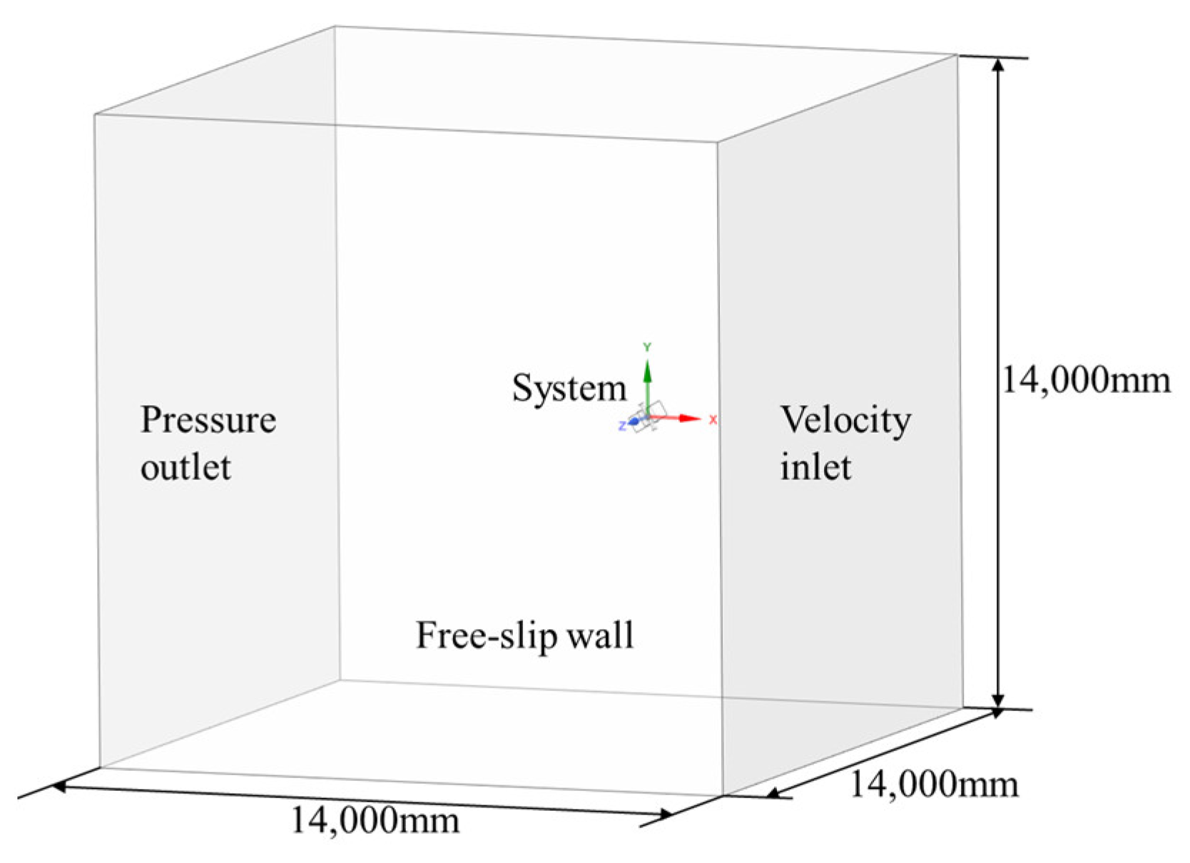
Preprocessing involves geometric model drawing, boundary condition definition, grid generation, and solver establishment. SpaceClaim (Version 2020 R2) was utilized for geometric simulation in a Cartesian coordinate system, with the origin set at the system’s center, as shown in Figure 4. The sailboard dimensions are set to 350 mm × 350 mm, the central bin height is 618 mm, the outer diameter is 132 mm, and the angle between the central axis and the X-axis can vary between 40° and 88°. The calculation domain is about 20 times the system’s feature length, measuring about 14,000 mm × 14,000 mm × 14,000 mm. Along the X-axis, the system center is positioned about 4400 mm from the entrance, and along the Y and Z axes, it is symmetrical about the interface on both sides. A 1000 mm × 1000 mm × 1000 mm cube around the system center serves as the mesh refinement area for higher quality mesh generation. The right boundary of the calculation domain is set as the velocity inlet, the left as the pressure outlet, and the other boundaries as free sliding walls. Fluent (Version 2020 R2) was utilized to generate the mesh, solving for the system’s resistance and buoyancy at varying inclination angles and ocean flow rates.

In the solution, gravity along the Y-axis is set to −9.81 m/s². The Reynolds number of the flow field around the system’s cross sail is between 8.517 × 10³ and 1.965 × 10⁴, indicating turbulence as the main factor. Thus, the k-epsilon model is chosen. The cell area contains liquid water with a density of 1020 kg/m³. Resistance and lift force are calculated by varying the inlet velocity corresponding to different flow velocities.

To ensure the accuracy of the solution, the grid independence of the model was verified. Five models with varying grid numbers, as shown in

Table 2. Simulation results of different models with varying grid numbers when ${\theta }_2$ = 60° and $V$ = 0.1 m/s.

Grid Number	${\mathit{F}}_{\mathit{d}}\left(\mathbf{N}\right)$	${\mathit{F}}_{\mathit{l}}\left(\mathbf{N}\right)$
647,036	1.4961	0.8084
1,310,304	1.4783	0.7986
2,130,535	1.4868	0.7996
2,803,653	1.4856	0.7990
3,832,179	1.4860	0.8001

, were assessed by solving $F_d$ and $F_l$ at ${\theta }_2=$ 60° and $V=$ 0.1 m/s. Table 2 shows no significant differences in solution results among the models with different grid numbers. For subsequent calculations in this study, the grid count was set to approximately 2 million.

Resistance and lift force are solved separately for different tidal flow velocities and incidence angles, resulting in data shown in

Table 3. Simulation results of different values of $V$ and ${\theta }_2$.

$\mathit{V}(\mathbf{m}/\mathbf{s})$	${\mathit{\theta }}_2(°)$	${\mathit{F}}_{\mathit{d}}\left(\mathbf{N}\right)$	${\mathit{F}}_{\mathit{l}}\left(\mathbf{N}\right)$	$\mathbf{Y}\left(\mathbf{N}\right)$
0.1	87	1.861	0.090	35.600
	80	1.817	0.311	10.616
	70	1.686	0.585	5.217
	60	1.487	0.801	3.377
	50	1.258	0.955	2.454
	40	1.180	0.984	1.974
	30	0.738	1.041	1.467
0.16	87	4.706	0.227	90.023
	80	4.656	0.798	27.203
	70	4.316	1.501	13.359
	60	3.826	2.074	8.701
	50	3.227	2.471	6.317
	40	3.018	2.541	5.073
	30	1.879	2.706	3.791
0.22	87	9.030	0.443	172.746
	80	8.841	1.515	51.655
	70	8.159	2.841	25.258
	60	7.253	3.939	16.502
	50	6.089	4.687	11.944
	40	5.706	4.827	9.615
	30	3.537	5.135	7.177
0.28	87	14.588	0.724	279.080
	80	14.267	2.447	83.359
	70	13.170	4.597	40.781
	60	11.692	6.349	26.600
	50	9.904	7.652	19.455
	40	9.247	7.839	15.598
	30	5.739	8.356	11.669
0.34	87	21.500	1.074	411.318
	80	20.938	3.594	122.339
	70	19.399	6.769	60.067
	60	17.259	9.374	39.267
	50	14.565	11.255	28.613
	40	13.630	11.565	23.002
	30	8.473	12.354	17.246

, where $Y$ is calculated using Equation (7).

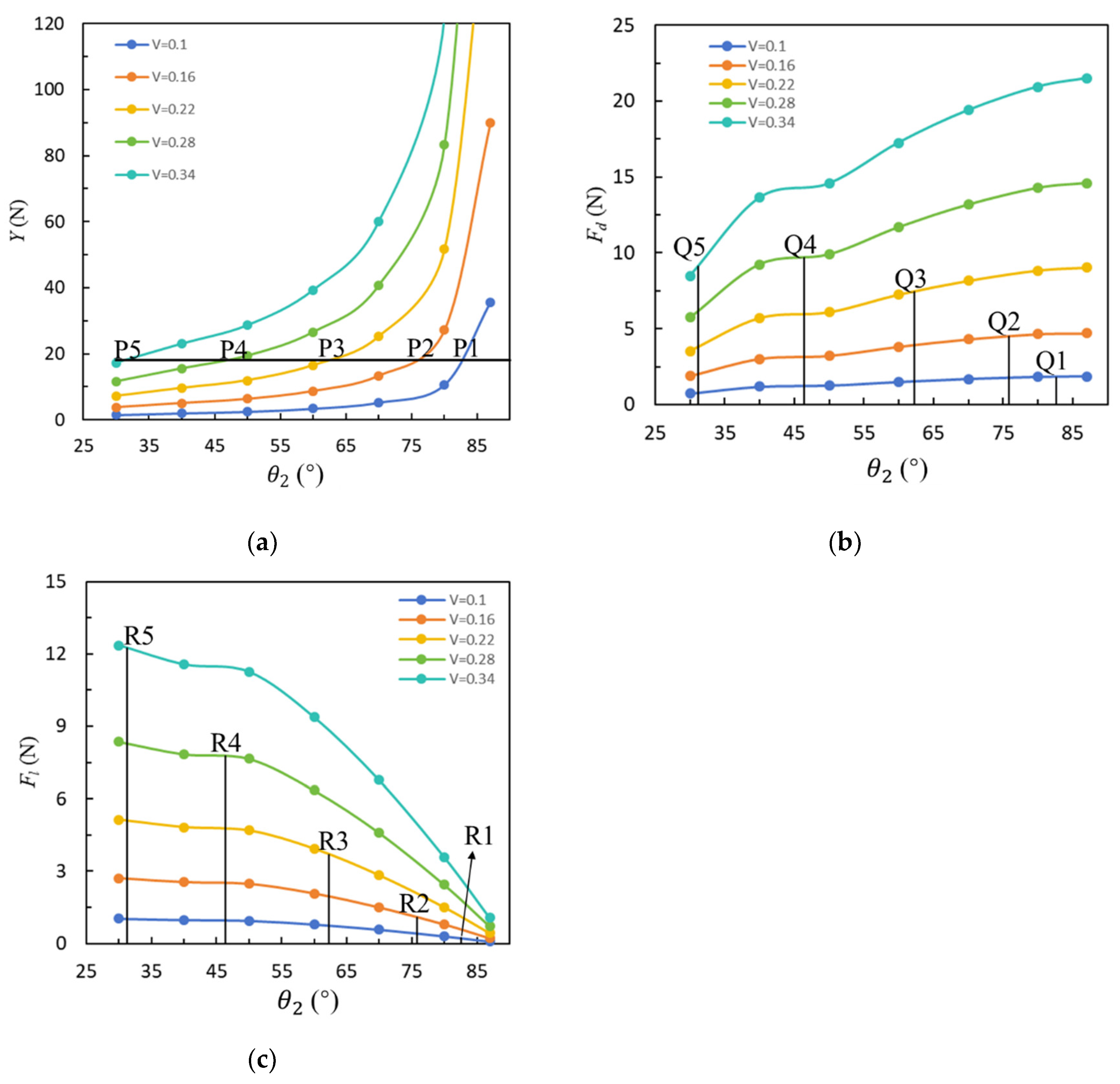
Based on the data in Table 3, Figure 5 can be drawn, which illustrates the relationship between $Y$, $F_d$, and $F_l$ at various values of $V$ and ${\theta }_2$.

To enhance tidal current energy conversion efficiency, the profiler is designed to achieve weak buoyancy (buoyancy slightly exceeds gravity) in water. Since $Y=F_f-G$, a smaller $Y$ indicates higher efficiency. A line $Y=18$ was drawn in Figure 5a, intersecting five curves at points P1 to P5. Theoretical ${\theta }_2$ was determined through image fitting. Figure 5b,c provide the corresponding $F_d$ and $F_l$ for each $V$ at the theoretical ${\theta }_2$, labeled Q1–Q5 and R1–R5, respectively. The coordinates are presented in

Table 4. The coordinates of points P1-P5, Q1–Q5 and R1–R5.

Points	Coordinates	Points	Coordinates	Points	Coordinates
P1	(82.634, 18)	Q1	(82.634, 1.789)	R1	(82.634, 0.219)
P2	(75.824, 18)	Q2	(75.824, 4.473)	R2	(75.824, 1.075)
P3	(62.234, 18)	Q3	(62.234, 7.422)	R3	(62.234, 3.692)
P4	(46.481, 18)	Q4	(46.481, 9.681)	R4	(46.481, 7.765)
P5	(31.232, 18)	Q5	(31.232, 9.084)	R5	(31.232, 12.232)

.

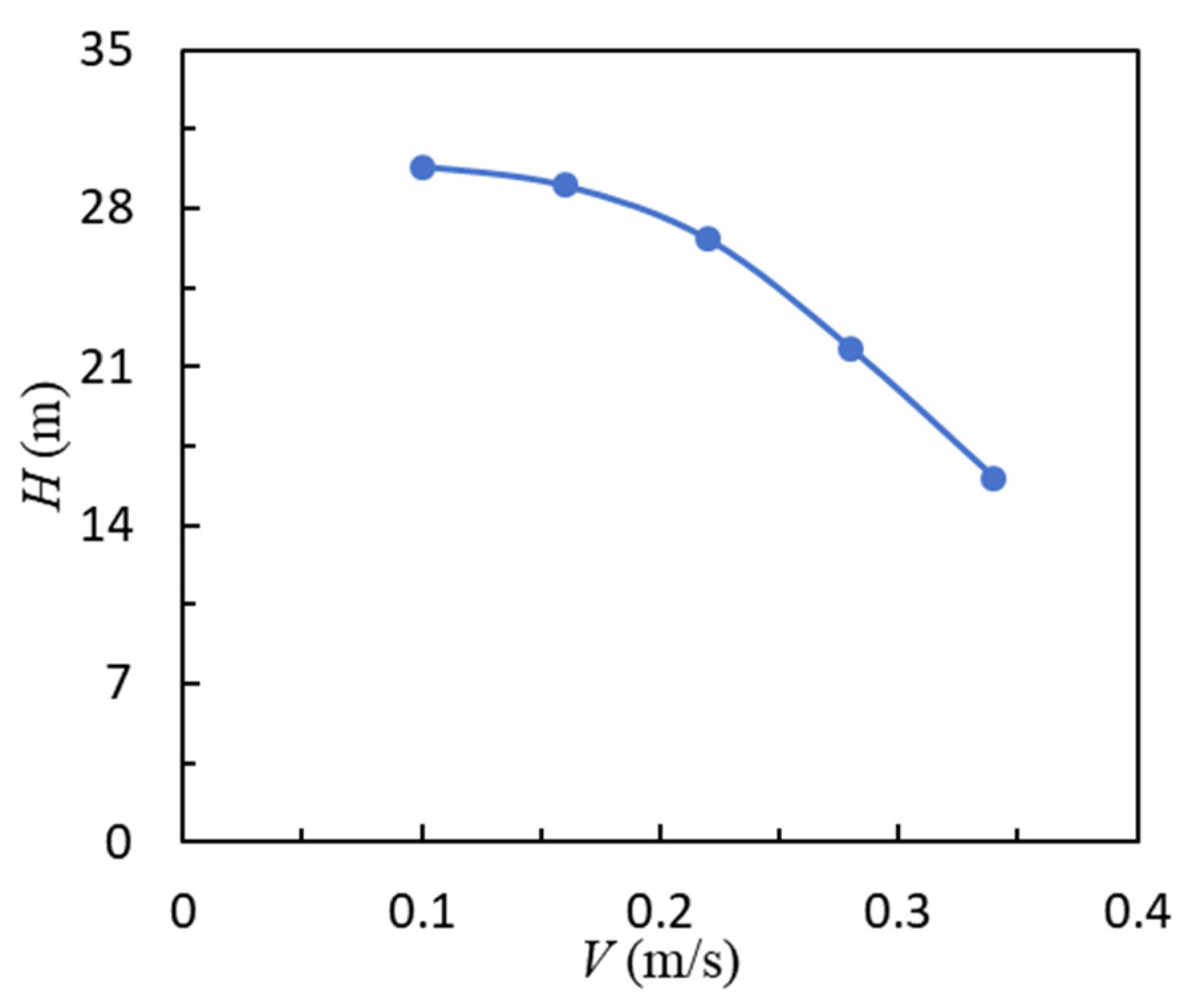
The design $L_{OB}=40$ m, and the corresponding $H$ is calculated using Equation (4) for each $V$ as shown in Table 4. Based on the data in

Table 5. The value of H at different values of V.

$\mathit{V}$ (m/s)	$\mathit{H}$ (m)
0.1	29.849
0.16	29.004
0.22	26.630
0.28	21.794
0.34	16.081

, Figure 6 can be drawn.

Data fitting reveals the relationship between $H$ and $V$.

$$H=-242.02V^2+48.579V+27.441$$

(8)

The simulation results, as shown in Figure 6, demonstrate that H decreases as V increases. This inverse relationship is consistent with the system’s design requirements, confirming that the system can effectively adjust its depth in response to tidal forces. Specifically, when the tidal current velocity is low, the system ascends to shallower depths, while higher tidal velocities drive the system to greater depths. This behavior is essential for achieving the desired vertical profiling range of 0–50 m, as outlined in the system’s design objectives.

The numerical simulations also provided valuable insights into the system’s performance under different tidal conditions, which were used to guide the selection of deployment sites and the setting of profiling depths during sea trials. For example, the results indicated that in regions with strong tidal currents, the system can achieve greater depths, making it suitable for monitoring deeper water columns. Conversely, in areas with weaker tidal currents, the system’s depth range may be more limited, requiring adjustments to the buoyancy regulation unit to achieve the desired profiling depths.

Overall, the numerical simulations not only validated the system’s design but also provided a theoretical basis for its deployment in various marine environments. The results confirmed that the system’s depth can be effectively controlled by tidal forces, ensuring its ability to perform continuous, high-resolution monitoring across the entire water column. This theoretical guidance was instrumental in planning the subsequent sea trials, where the system’s performance was further validated under real-world conditions.

2.2.2. Buoyancy Regulation Principle

In the actual marine environment, current velocity is influenced by factors such as geographical locations, the relative positions of the Earth, Moon, and Sun, offshore distance, and surrounding terrain. These factors may affect whether the current can always drive the system to move within the required depth range. For example, in China, Hangzhou Bay, a strong tidal region, exhibits a surge velocity range of 1.85–2.79 m/s and a fall velocity range of 1.44–2.35 m/s during spring tides [19]. 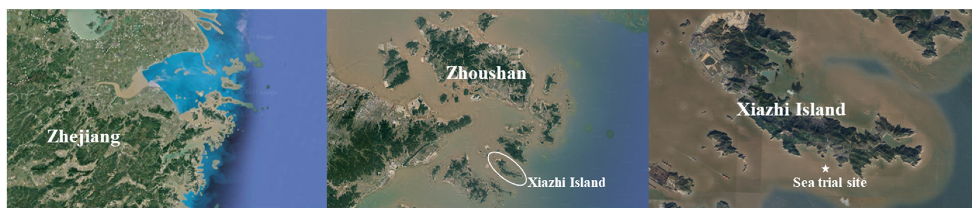In Aoshan Bay, Shandong Province, the maximum rising tidal current velocity is 0.72 m/s, while the maximum falling tidal current velocity is 0.65 m/s [20]. Even within the same region, tidal current velocity varies with the moon’s phases. During neap tides near the channel of Xiazhi Island, Zhoushan, Zhejiang Province, the average flow velocities of high tide and low tide are 0.50 m/s and 0.46 m/s, respectively. 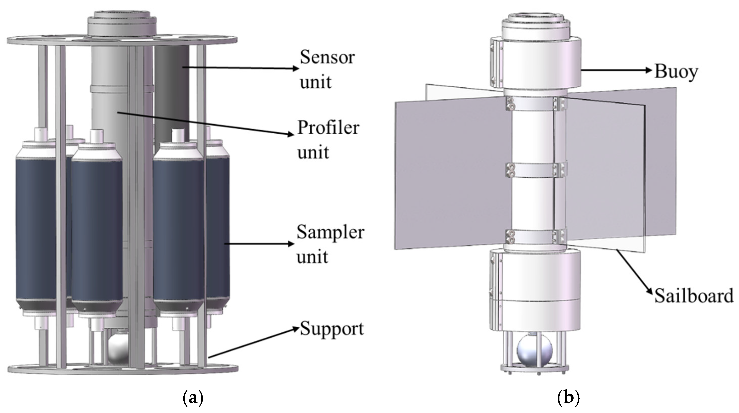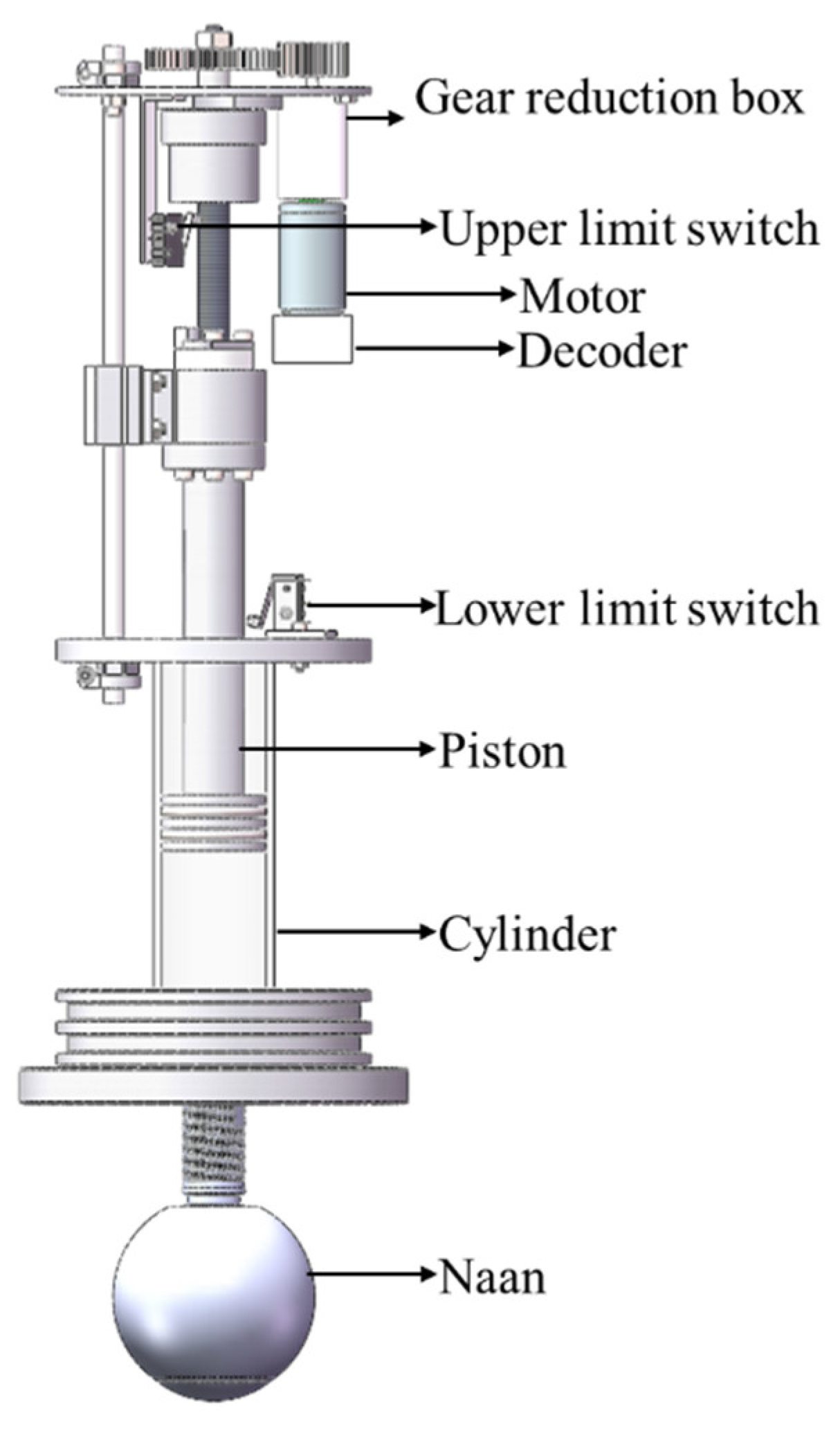During spring tides, the average rising tide velocity is 0.58 m/s, while the average falling tide velocity is 0.69 m/s [21]. To enable practical application, relying solely on tidal flow energy would limit the profiler’s offshore usability. Thus, a buoyancy regulation unit, as illustrated in Figure 7, is incorporated in the system.

A pressure sensor on the upper end cap of the profiler measures the system’s depth. When tidal flow cannot drive the system to the specified depth, the buoyancy regulation unit actively adjusts buoyancy to enable controlled floating and sinking. The buoyancy regulation unit uses a decoder for data transmission with the MCU, which controls motor rotation. The motor reduces speed via a gear reduction box, driving the piston up or down to push oil into or out of the cylinder. This process increases or decreases buoyancy, enabling the system to float or sink. A limit switch restricts the piston rod’s movement range, preventing overextension.

2.2.3. Parameter Monitoring

The sensor unit monitors parameters such as currents, chlorophyll levels, nutrient concentrations, temperature, and salinity across different depths. Currents are measured using a current meter, while a CTD device records temperature, salinity, and depth, and a YSI sensor measures chlorophyll levels and nutrient concentrations.

2.2.4. Sample Collection Principle

The sampler unit uses a cap-type sampler [22] consists of a bottle body, upper and lower covers, O-rings, a rubber band, and a traction rope. The bottle body serves as the main structure of the water sampler, storing collected water samples and supporting other components. A rubber band connects the upper and lower covers. Initially, the traction rope is tightened to keep the upper and lower caps open. When the system reaches the specified depth, the motor releases the pull ring, allowing the rubber band’s tension to close the upper and lower caps, completing sample collection. The construction of the sampler bottle is shown in Figure 8.

The sealing mechanism of the water sampler relies on the tension provided by the deformation of a rubber band. This tension causes the bottle cap and the bottle body to compress against each other, deforming the O-ring to close the gap between the cap and the body. Once the water sampler is closed underwater, it becomes filled with seawater, equalizing the internal and external pressure of the sampler. As a result, pressure changes caused by the sampler’s depth variation in seawater do not lead to sample leakage or external seawater infiltration. After the sampler is brought to the surface, the rubber band must provide sufficient tension and ensure proper deformation of the O-ring to prevent sample leakage.

The elasticity of the rubber band is calculated using Hooke’s Law.

$$F_t=kx$$

(9)

where $F_t$ is the force, $x$ is the elongation of the rubber band, and $k$ is the stiffness coefficient. The stiffness coefficient $k$ depends on the length $L$ and cross-sectional area $S$ of the untensioned rubber band. The relationship is given by:

$$k={\displaystyle \frac{Y^{\prime }}{L}}S$$

(10)

where $Y^{\prime }$ is the Young’s modulus of the material.

The rubber band, with a Young’s modulus of $Y^{\prime }=$ 1.5 MPa, is designed as a ring with a circumference of 400 mm and a square cross-section with a width of 10 mm and a thickness of 4 mm. Using these parameters, the stiffness coefficient $k=$ 150 N/m is obtained.

After the upper and lower covers of the water sampler are closed, the length of the rubber band increases to approximately 700 mm. Therefore, the elastic force of the rubber band is 45 N, and the tension on the upper and lower covers is 90 N. After the water sampler is filled with seawater, the weight of the seawater inside is approximately 2.5 kg, and the weight of the lower end cap is about 0.2 kg. This results in a force of approximately 63.5 N being applied to the O-ring.

The O-ring is made of soft rubber, with a wire diameter of 3.6 mm and an inner diameter of 61.4 mm. The groove width is 5 mm, and the groove depth is 3 mm. Under the applied force, the O-ring compresses by 0.6 mm, ensuring that the lower cap fits tightly against the bottle body.

The pressure on the O-ring due to the seawater can be calculated using the formula:

$$P=\rho g{h}_s$$

(11)

where $P$ is the pressure, $\rho =$ 1020 kg/m³ is the density of seawater, $g=$ 9.81 m/s² is the acceleration due to gravity, and $h_s$ is the height of the liquid. The calculated pressure is approximately 3602.23 Pa.

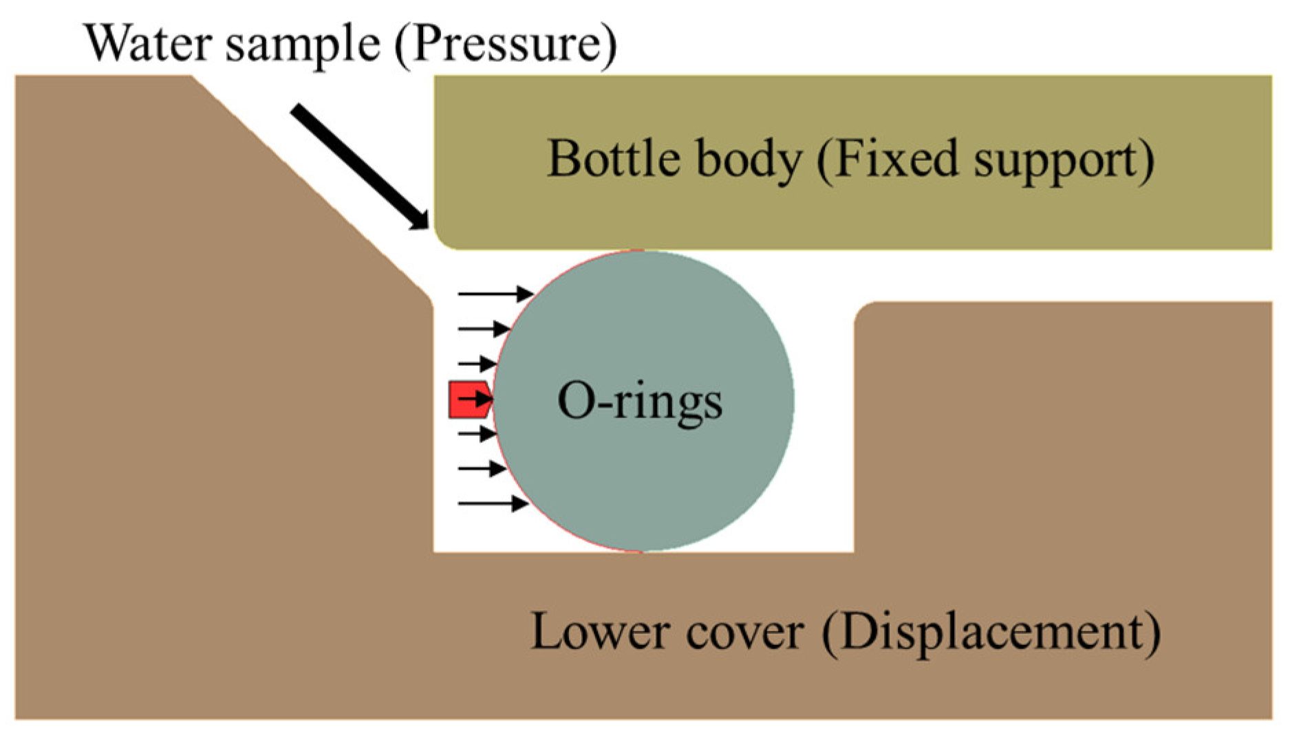
To theoretically validate the feasibility of the water sampler’s design, ensuring that it can effectively collect and preserve water samples without leakage, simulations were performed using ANSYS Workbench (Version 2020 R2) [23]. The model design is shown in Figure 9. The simulations analyzed the deformation and contact pressure of the O-ring under different internal pressures, providing insights into the sealing effectiveness under real-world conditions.

Figure 10 illustrates the deformation and contact surface pressure of the O-ring after the bottle cap is closed and internal pressure is applied. The simulation results show that the maximum deformation of the O-ring is approximately 0.6 mm, with no significant lateral displacement observed. Additionally, the contact pressure exceeds the medium pressure, confirming that the O-ring provides an effective seal.

2.3. Control Strategy of the System

The system control strategy is primarily designed to manage the profiler unit and the sample collection unit. Through active control, the profiler unit can actively float and sink when the power flow is insufficient, and the sampler unit can collect water samples at various depths and times. The algorithm environment of the system’s main program is shown as follows (Algorithm 1):

Algorithm 1 Main Program

1: Start

2: Check modeselect

3: if modeselect == 0:

4:      Execute Sampler Program

5:      End

6: else

7:      Execute Reset Program

8:      Initialize variables: i = 0; n = n0 (predefined value)

9:      while i != n do

10:          i++

11:          Delay execution for ti (predefined value) seconds

12:          if i%2 != 0

13:              Execute Floating Program

14:          else

15:              Execute Sinking Program

16: End

In the main program, after powering on, the system selects either long-term monitoring or sample collection based on the modeselect setting, then jumps to the corresponding subroutine. During long-term monitoring, the system is set to perform n0 cycles of ascent and descent based on monitoring requirements. The system first runs a reset program to maintain initial buoyancy. It then moves under tidal forces, continuously recording data. Delays are used to ensure that the floating program and sinking program are executed at minimum and maximum tidal flow, respectively, with timing determined by deployment and tidal conditions. The program executes ascent and descent cycles sequentially, ending after completing the set number of cycles.

The reset program (Algorithm 2), floating program (Algorithm 3), and sinking program (Algorithm 4) are illustrated as follows. The reset program primarily functions to restore the system’s buoyancy to its initial state. Based on the above working principles, when the power flow velocity is at its minimum, the system depth is at its shallowest, making it likely to approach the upper monitoring limit. At this point, the floating program is executed. Similarly, when the tidal current velocity is at its maximum, the system reaches its greatest depth, making it likely to approach the lower monitoring limit. At this point, the sinking program is executed.

Algorithm 2 Reset Program

1: Start

2: if Upper Limit Switch triggered

3:      Rotate motor m (predefined value) turns Clockwise

4: else if Lower Limit Switch triggered

5:      Rotate motor n (predefined value) turns Counter-Clockwise

6: else

7:      while Upper Limit Switch not triggered do

8:          Rotate motor continuously in Counter-Clockwise

9:      Rotate motor m (predefined value) turns Clockwise

10: End

Algorithm 3 Floating program

1: Start

2: Get current depth H

3: if H > Ht (predefined value)

4:      End

5: else

6:      while Upper Limit Switch not triggered do

7:          Rotate motor continuously in Counter-Clockwise

8:      Continuously check whether H > Ht for t (predefined value) minutes

9:          if H > Ht

10:              Execute Reset Program

11:              End

12:    Execute Reset Program

13: End

Algorithm 4 Sinking program

1: Start

2: Get current depth H

3: if H < Hb (predefined value)

4:      End

5: else

6:      while Lower Limit Switch not triggered do

7:          Rotate motor continuously in Clockwise

8:      Continuously check whether H < Hb for t (predefined value) minutes

9:          if H < Hb

10:            Execute Reset Program

11:              End

12:      Execute Reset Program

13: End

The sampler unit is employed to collect water samples at various depths. The system ascends or descends gradually under the traction of the winch, while the MCU reads the depth from the pressure sensor. When the system reaches the preset depth, the MCU sends a signal to activate the electronic switch, causing the motor to rotate, the traction rope to loosen, and the rubber band to contract, sealing the water sampler bottle cap (Algorithm 5).

Algorithm 5 Sampler program

1: Start

2: Initialize variables: i = 0, n = n1 (predefined total number of motors)

Define H as a predefined array of depth values: H[0], H[1], …, H[n − 1]

3: while i < n do

4:      Continuously monitor the current depth

5:          if H = H[i]

6:              Rotate Motor number “i” for t (predefined value) seconds

7:              i++

8: End

3. Experimental Setup and Methods

The system was set up as illustrated in Figure 11.

The electrical and control connections of the system are illustrated in Figure 12. The battery pack powers the entire system via a power supply board. The battery pack comprises 12 lithium batteries (3.6 V each, nominal capacity: 2500 mAh), providing a total energy capacity of 0.108 kWh. A rotary switch, installed externally on the pressure-resistant enclosure, enables system power control. The battery is rechargeable via waterproof connectors. The MCU communicates with the motor control module via RS232 to regulate the piston motor, adjusting system buoyancy. The MOSFET module assists the MCU in activating/deactivating six water sampler motors (Motor 1–6) to collect samples. Sensor data are stored on an SD card integrated with the MCU. After equipment retrieval, the PC can reprogram the MCU and retrieve data from the SD card via waterproof connectors. Further data processing is conducted on the PC.

The verification experiments included both pool tests and sea trials. The pool tests were conducted to verify the system’s tightness, perform gravity trimming of the profiler unit, calibrate the pressure sensor, and test the buoyancy regulation and sampler units. The sea trials aimed to verify the system’s ability to perform reciprocating vertical movements driven by tidal energy as demonstrated in numerical simulations, validating its feasibility for long-term, continuous monitoring, and to verify the system’s ability to collect water samples at various depths.

The pool experiments were conducted at Yuanchi Hall in the Zhoushan Campus of Zhejiang University. First, the equipment’s tightness was tested by installing only the external sealing bin and submerging the equipment at the bottom of the pool for 24 h. No leakage was observed, after which the internal electronic components were installed for subsequent experiments.

In the gravity trimming experiment, the equipment was initially adjusted to a weak buoyancy state in seawater. PMI buoyancy materials were installed externally to slightly increase the equipment’s buoyancy above its gravitational force. The piston was then reset, the equipment was placed in the pool, and steel studs were added until the equipment achieved a weak buoyant state.

The pressure sensor calibration experiment was conducted to verify the accuracy of its pressure output. The piston was controlled to compress the oil naan causing the equipment’s gravity to exceed its buoyancy. A lead rope was used to lower the equipment gradually. Each meter along the rope was marked with a rolling strip. The sensor was configured to record data every second, and the equipment was held at a position where the pressure sensor first entered the water for 10 min. This position was defined as the depth of 0 m. The equipment was then gradually lowered, pausing 3 to 4 min at each marked location until it reached near the bottom. After completing the experiment, the data were explored and processed to verify the normal operation of the pressure sensor.

The buoyancy regulation experiment was conducted to verify whether the equipment could independently sink and float in water. The total control program delay time was set to 5 min, and n0 = 6. The floating and sinking procedures were modified by removing the step of depth judgment after initiation, allowing the motor to directly start floating or sinking. The program was entered into the equipment, and observations were made to ensure the naan contracted and expanded as expected. After completion, the equipment was placed into the water to observe whether the system could automatically sink and float three times as per the program settings.

The sampler unit experiment was conducted to verify whether the equipment could collect water samples at specific depths. First, the program was verified on the surface by configuring samplers No. 1 to No. 6 to close every two minutes. Observations were made to ensure the motor operated as configured and that the sampler bottle caps closed properly. Once this was verified, the underwater experiment was conducted. The sample collection program was configured with H0 to H5 set to depths of 1 m, 2 m, 3 m, 4 m, 5 m, and 6 m, respectively. A marked lead rope was used to gradually lower the equipment until it approached the pool’s bottom. The equipment was then retrieved, and observations were made to verify whether the sampling was complete and if any leaks were present.

The sea trials were conducted as shown in Figure 13. During the water sample collection test, the equipment is slowly lowered using the ship’s winch, and it automatically collects water samples at the specified depth. For long-term monitoring tests, the system is connected to a seabed anchor with a cable, and its depth changes in response to variations in current speed, allowing for the recording of parameter data at different depths. When tidal currents are insufficient to drive the system to the specified depth, the system adjusts its buoyancy to ascend or descend accordingly. Additionally, during long-term monitoring, a buoy is tethered to the anchor via a cable. The buoy serves as a visual warning to prevent vessels from approaching the device and aids in locating the system for retrieval.

4. Results and Discussion

4.1. Pool Experiments

In the pool experiment, no water leakage occurred after the equipment was submerged, and its sealing performance met the system’s seawater work within 50 m. After the buoyancy material was installed, the equipment was adjusted to a state of weak buoyancy by adding a counterweight. Figure 14a illustrates the variation in pressure values recorded during the pressure sensor calibration experiment over time.

Figure 14a reveals six plateau periods, attributed to the equipment remaining at the cable mark for 3–4 min during the experiment. The average pressure values during each plateau period were calculated, correlated with the corresponding water depth, and used to fit the curve of pressure variation with depth, as shown in Figure 14b. The water depth, $D$ (in meters), and pressure, $P$ (in millibars), satisfy Equation (12).

$$D=0.01056P-9.927$$

(12)

During the buoyancy control test, the equipment was observed to independently sink and float in the water. The depth exhibits three downward and upward trends, consistent with the observed results, demonstrating that the buoyancy regulation unit can effectively adjust the system’s buoyancy, enabling the equipment to independently ascend and descend in the water.

In the sample collection unit validation, it was observed that as the system descended to greater depths, the sampler sequentially closed at the specified depths. Upon the system’s retrieval to the surface, no sample leakage was detected in the sampling bottles. This demonstrates that the sampling unit is capable of collecting samples at the designated depths, and the sealing of the sampling bottles ensures that the sample does not leak.

The results of pool experiments demonstrated that the system achieved a watertight seal, maintained neutral buoyancy, and successfully collected water samples at predefined depths. The pressure sensor calibration confirmed the accuracy of depth measurements, with a linear relationship between pressure and depth, as shown in Figure 14b. The buoyancy regulation unit effectively adjusted the system’s depth, enabling it to ascend and descend autonomously, as illustrated in Figure 15.

4.2. Sea Trials

The sea trials were conducted in the coastal waters near Xiazhi Island, Zhoushan City, Zhejiang Province, China (122°16′40.60″ E, 29°43′44.96″ N), as shown in Figure 16. The tidal regime in this area is characterized by an irregular semi-diurnal tide, with an average flood tide velocity ranging from 0.35 to 0.63 m/s and an average ebb tide velocity ranging from 0.48 to 0.73 m/s.

First, a sample collection test was conducted. The sample collection unit was installed on the system, and the system was slowly lowered using a winch, as illustrated in Figure 13a. During the descent, the system automatically collected samples. Upon reaching the specified depth, the system was retrieved. After retrieval, all sampling bottles were found to be securely closed, and the samples were successfully obtained, indicating the smooth completion of the test. Deployment process of the sea trials is shown in Figure 17.

The long-term monitoring experiment lasted approximately 19 h; the specific time periods of flood and ebb tides during these 19 h are detailed in

Table 6. The specific time periods of flood and ebb tides and program initiation times.

Flood/Ebb Tide	Time Period	Program	Initiation Times
Ebb tides	14:00 PM–21:15 PM	Sinking program	17:37 PM
Flood tides	21:15 PM–5:20 AM	Floating program	21:19 PM
		Sinking program	01:25 AM
Ebb tides	5:20 AM–11:20 AM	Floating program	05:41 AM

. According to the designed control strategy, the descent procedure was initiated at 17:37 on the first day and at 01:25 on the second day, while the ascent procedure was activated at 21:19 on the first day and at 05:41 on the following day.

During the marine experiment, the sampling frequency of the pressure sensor and temperature sensor was set to 1 s. Data collection commenced at 16:59:48 and concluded at 09:53:38 the following day, resulting in a total of 60,879 sets of pressure and temperature data being acquired. After processing the collected data, Figure 18 was plotted.

The monitoring system’s upper limit was set to 8 m, and the lower limit was set to 27 m. In Figure 18, the initiation times of the procedures are marked on the horizontal axis. Throughout the experiment, a total of six complete ocean profile parameters were measured, demonstrating that the system could achieve reciprocating movements within the water column.

During the ebb tide period (14:00 to 21:15), the tidal current velocity followed a predictable pattern: it began to increase at 14:00, reached its maximum around 17:37, and then gradually decreased until 21:15. According to the numerical simulation results, the system’s depth should reach its maximum at 17:37, followed by a gradual ascent as the tidal current velocity decreases. This behavior is clearly reflected in the experimental data, as shown in Figure 18. The system’s depth increased as the tidal current velocity rose, reaching its maximum depth around 17:37, and then decreased as the current velocity declined, demonstrating a strong correlation between tidal energy and the system’s vertical movement.

Similarly, during the flood tide period (21:15 to 5:20), from 21:15 to 01:25, the tidal current velocity increased, causing the system to descend and reach its maximum depth around 01:25. As the current velocity decreased from 01:25 to 05:41, the system gradually ascended, with its depth decreasing accordingly. The experimental data closely matched the predicted behavior based on the numerical simulations, confirming the system’s ability to respond to tidal forces and achieve the desired profiling depths.

The system’s buoyancy regulation unit played a critical role in ensuring that the system reached the specified monitoring depths when tidal currents alone were insufficient. As shown in Figure 18, the system’s depth occasionally deviated from the expected profile due to variations in tidal current velocity. In such cases, the buoyancy regulation program was activated to adjust the system’s buoyancy, enabling it to reach the preset depth. For example, at 17:37, the system had already reached the target depth, so the buoyancy regulation program was not activated. However, at other times, such as 21:19 and 05:41, the program was initiated to ensure that the system achieved the desired depth, demonstrating the effectiveness of the buoyancy regulation mechanism.

In addition to depth and temperature data, the system’s energy consumption (mainly consumed by motor rotation of buoyancy regulation) was recorded by measuring the motor current at 1 s intervals. With a motor voltage of 24 V, the energy consumption was calculated using the following formula:

$$W=\sum UI∆t$$

(13)

where $W$ is the energy consumption of the system, $U$ is the voltage of motor, $I$ is the current of motor, and $∆t=1\mathrm{s}$ is the running time of the motor.

The total energy consumption during the experiment was 3.204 × 10⁻⁴ kWh; for every 100 m in the vertical direction, the electrical energy consumed is 1.71 × 10⁻⁴ kWh. This is a big improvement over traditional profiling platforms such as the MMP (2.16 × 10⁻⁴ kWh per 100 m [7]) and the AMP (4.16 × 10⁻³ kWh per 100 m [8]), which rely solely on electrical power for buoyancy regulation and vertical movement. Additionally, the buoyancy regulation unit provides greater flexibility in depth control compared to OTP and WW, while the sampler unit enables detailed sample collection, complementing the sensor-based monitoring capabilities. These advantages position our system as a versatile and cost-effective tool for a wide range of marine research and monitoring applications.

5. Conclusions

This study develops an autonomous ocean observation system driven by tidal energy, integrating sensor-based monitoring and sample collection for continuous marine profiling. Validated through lab and sea trials, the system achieves vertical reciprocating movements in 0–30 m of water under tidal influence for six times and autonomously adjusts buoyancy to reach specified depths when tidal currents are insufficient. A key innovation of this system is its tidal energy-driven capability, which significantly reduces reliance on electrical power (1.71 × 10⁻⁴ kWh per 100 m of vertical movement) compared to traditional platforms such as Argo floats, MMPs, and AMPs. This makes the system more energy-efficient and suitable for long-term monitoring. The inclusion of a buoyancy regulation unit further enhances the system’s flexibility, allowing for precise depth control and adaptability to varying tidal conditions. Additionally, the system’s integration of sensor-based monitoring with sample collection provides a complementary approach to marine research. This dual capability allows for a more comprehensive understanding of marine ecosystems, combining the strengths of both approaches and expanding the system’s potential applications in environmental monitoring, ecological research, and resource management. Results confirm the system’s viability as a cost-effective, sustainable solution for ocean monitoring. Future work may optimize energy efficiency and expand deployments. This research advances tidal energy-driven technologies, enhancing marine ecosystem understanding and conservation efforts.