The Application of a Joint Distribution of Significant Wave Heights and Peak Wave Periods in the Northwestern South China Sea

Abstract

A joint distribution of significant wave heights ($H_s$) and peak wave periods ($T_p$) in the northwestern South China Sea is created using a conditional distribution model in this work. An unstructured triangular mesh wave model covering the northwestern South China Sea is established based on the third-generation spectral wave model SWAN. This wave model has been extensively validated against field data and was run from 1979 to 2020 to generate long enough one-hourly $H_s$ and $T_p$. Four probability density functions including Normal, Lognormal, Gamma and 3P Weibull distributions are adopted to construct the marginal independent distribution of $H_s$. The results show that the 3P Weibull distribution is more suitable in fitting the marginal distribution of $H_s$ compared to the other three distributions. Three combinations of dependence functions ($\mu \mathrm{and} \sigma$), namely, power3 and exp3, insquare2 and asymdecrease3, and logistics4 and alpha3, are used to create the Normal and Lognormal distributions for $T_p$. The estimations of dependence functions and corresponding fitted $T_p$ demonstrate that the $\mu \mathrm{and} \sigma$ using power3 and exp3 perform best in producing the conditional distribution of $T_p$. In addition, the environmental contours derived by an IFORM are used to generate the extreme sea states with return periods of 1, 5, 10, 25, 50 and 100 years.

1. Introduction

Wave parameters (significant wave height and peak wave periods) observed in coastal and ocean areas are expected to have a relationship [1]. The existing univariate distribution methods using Pearson Ⅲ, Gumbel and Weibull distributions to fit single metocean parameters have limitations in analyzing the characteristic values of wave parameters. Joint environmental models are required for the assessment of the relative importance of various wave parameters and establishment of design load conditions for different limit states [2]. Different approaches for establishing a joint probability distribution (JPD) model exist.

For the short-term joint distribution of wave heights and periods, Longuet-Higgins [3] proposed a theoretical expression of the JPD between the wave heights and periods based on the hypothesis of a narrow spectrum. The shape of the joint probability density stated by Longuet-Higgins in 1975 is symmetric on $\tau ={\tau }_{mean}$ and indicated by ‘cocked hat’ curves with the wave periods becoming broader at a smaller height. A new asymmetric analytic expression [4], which fits better with real wave data, was derived by Longuet-Higgins for the JPD of wave heights and periods after introducing a new normalized factor to these parameters. Sun [5] also derived a JPD of wave heights and periods based on the linear model of sea waves and the ray theory of waves; this expression has the same merits as those of Longuet-Higgins, but the wave height distribution used is still Rayleigh’s. Zheng et al. [6] studied the difference between the JPD of the apparent wave heights and periods and the individual waves and improved the theoretical expression of the JPD, showing better performance in fitting the field data at large band widths, particularly. In addition, some other JPDs have been proposed as modifications of Longuet-Higgins [7,8]. Stansell et al. [7] took into account the idea that small waves are likely to have shorter periods than large waves and derived a new expression for the joint and marginal distributions of wave envelope amplitude and local wave period. Zhang et al. [8] modified the Longuet-Higgins formula by replacing the mean frequency with the peak frequency of the wave spectrum. James and Panchang [9] conducted a robust assessment of the available theoretical distribution models utilizing wave measurements around the UK coast and recommend that the Zhang and Guedes Soares model generally performs the best.

For the long-term joint distribution of wave height and period, various models have been established to analyze JPD. The maximum likelihood model [10] and the conditional modeling approach [11] require all available data from long-series observations of the environmental variables. The maximum likelihood model uses a Gaussian transformation of a simultaneous dataset, while the conditional modeling approach is defined as the product of a marginal independent distribution function and a conditional dependent distribution function. The predictions of extreme sea states obtained from the maximum likelihood model and the conditional modeling approach show similar values [12]. On the other hand, a copula-based model suggested by Salvadori et al. [13] may also be used to construct joint distribution models, which are based on a marginal distribution and a copula describing the dependence structure.

Previous studies show that considerable focus has been placed on the application and comparison of various joint distribution models, among which more achievements are about wave height than wave period. However, fewer assessments have been conducted on the dependence functions for conditional modeling approaches, which are very significant for the performance of joint distribution models. The present study aims to establish a joint distribution model of significant wave heights (SWHs, $H_s$) and peak wave periods (PWPs, $T_p$) in the northwestern South China Sea (SCS); furthermore, three combinations of dependence functions will be employed in the conditional distribution functions.

This study is organized as follows: Section 2 introduces the observational data used to validate the wave model and the details of the wave model configuration and validation. The typically used univariate distribution methods and combinations of dependence functions considered here are described in Section 3. In Section 4, the estimations of four marginal distributions for $H_s$, three combinations of dependence functions and corresponding conditional distributions for $T_p$ are discussed, along with a description of the environmental contours and extreme sea states. This study is summarized in Section 5.

2. Observational Data and Wave Model Configuration

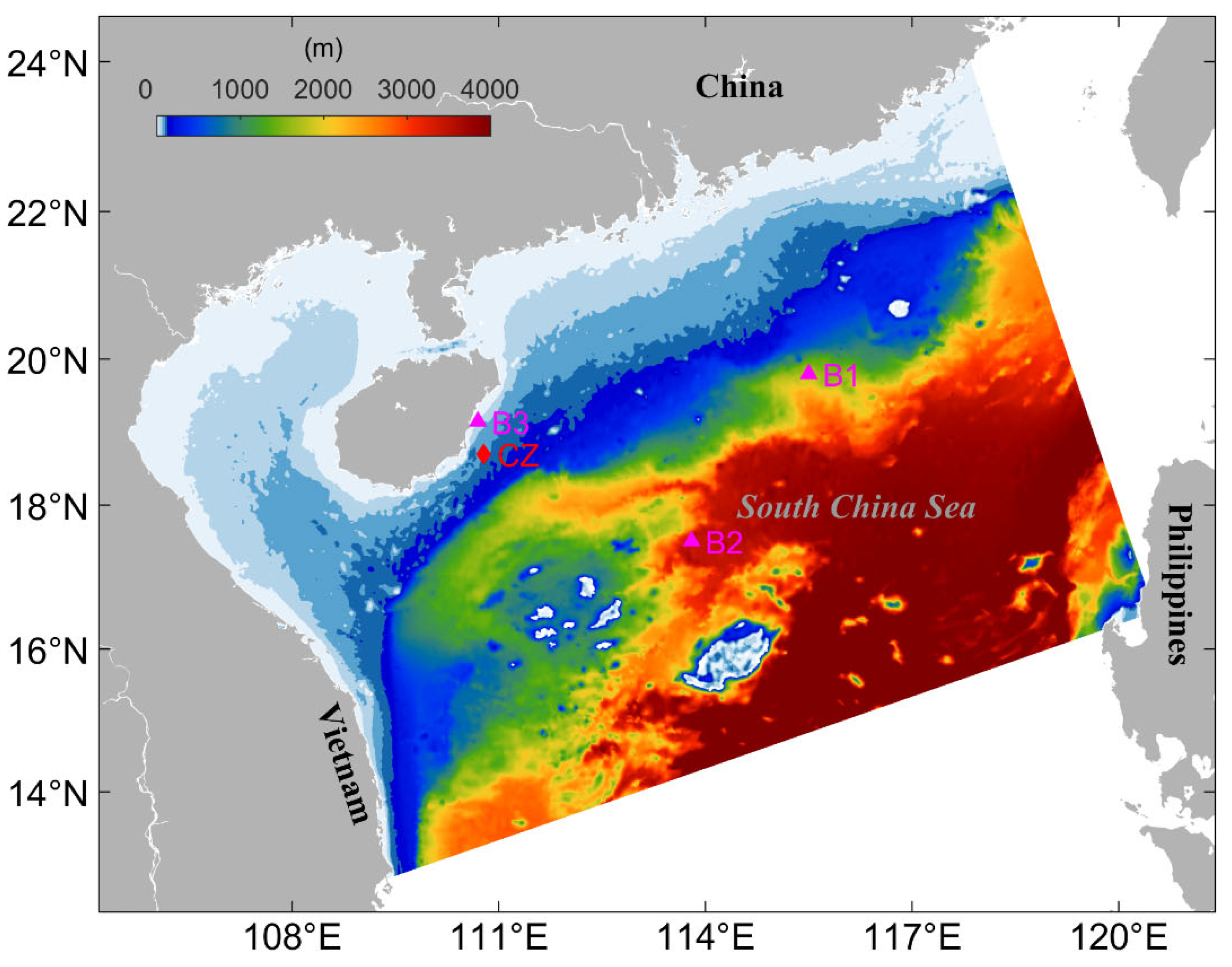
2.1. Observational Data

The in situ observations used in this study include $H_s$ and $T_p$, which were measured by wave rider buoys at stations B1 (115.7° E, 19.8° N), B2 (114.0° E, 17.5° N) and B3 (110.9° E, 19.2° N) between October and December 2019. The water depths of the B1, B2 and B3 stations are about 1750 m, 3450 m and 40 m, respectively. These observational data are quality-controlled and used to assess the accuracy of the northwestern SCS wave model.

2.2. Wave Model Configuration

The datasets used to analyze the extreme environmental parameters acting on the marine structures should cover a long enough time period to ensure the rationality of the results. It is usually difficult to obtain long-term field observations due to the destruction caused by humans and nature. Therefore, numerical simulations which were extensively validated against quality-controlled field data are a good choice of marine environmental datasets. A wave model based on the third-generation spectral wave model SWAN is established in this study. The domain of this wave model covers the northwestern SCS between 105.5° E and 120.5° E and between 12.6° N and 24.0° N (Figure 1). The model bathymetry with a resolution of 0.5′ is based on the General Bathymetric Chart of the Oceans (GEBCO, https://download.gebco.net/, accessed on 15 June 2024). This wave model is discretized using unstructured triangular meshes with the horizontal resolution ranging from 1 km to 20 km. The horizontal resolution near the coastal area is refined in this wave model.

The wind force used to drive this wave model is from the European Center for Medium-Range Weather Forecasts reanalysis (ERA5, https://cds.climate.copernicus.eu/datasets, accessed on 1 July 2024). ERA5 wind data with a horizontal resolution of 0.25° are available at one-hour intervals. The initial condition in this wave model is by default a JONSWAP spectrum with a cos²(θ) direction distribution centered around the local wind direction [14]. We assume that there are no waves entering the area and that waves can leave the area freely. Because the open boundaries are sufficiently far away from the study area, the computational results are thought to be reliable after extensive validation against observations.

This northwestern SCS wave model was run from 1979 to 2020 at the National Supercomputer Center to generate sufficiently long-term wave variables. The $H_s$ and $T_p$ at buoys B1, B2 and B3 are obtained from wave model results and compared to the observational data. The simulated long series of $H_s$ and $T_p$ at station CZ are used as the characteristic wave data of the northwestern SCS to analyze the joint distribution models.

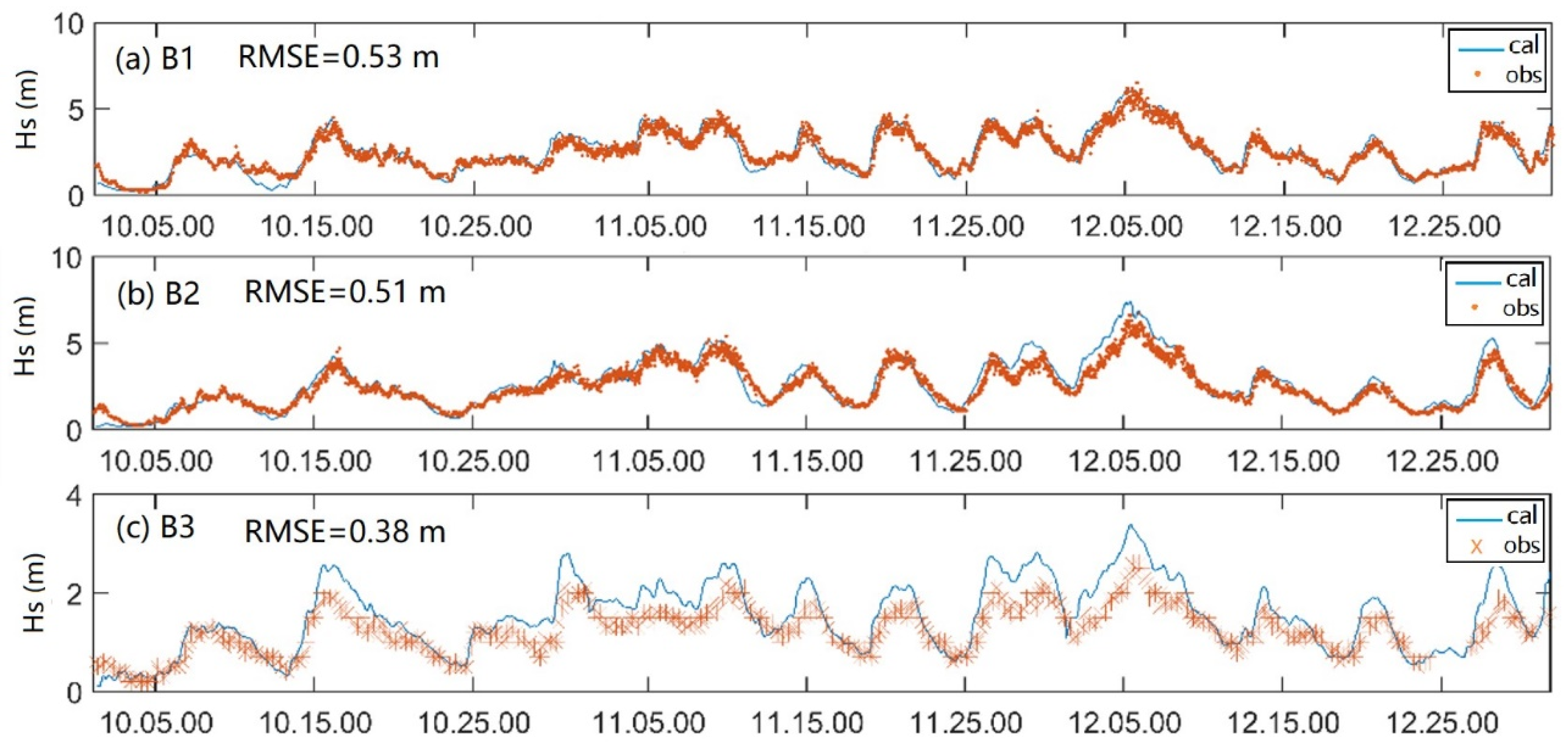
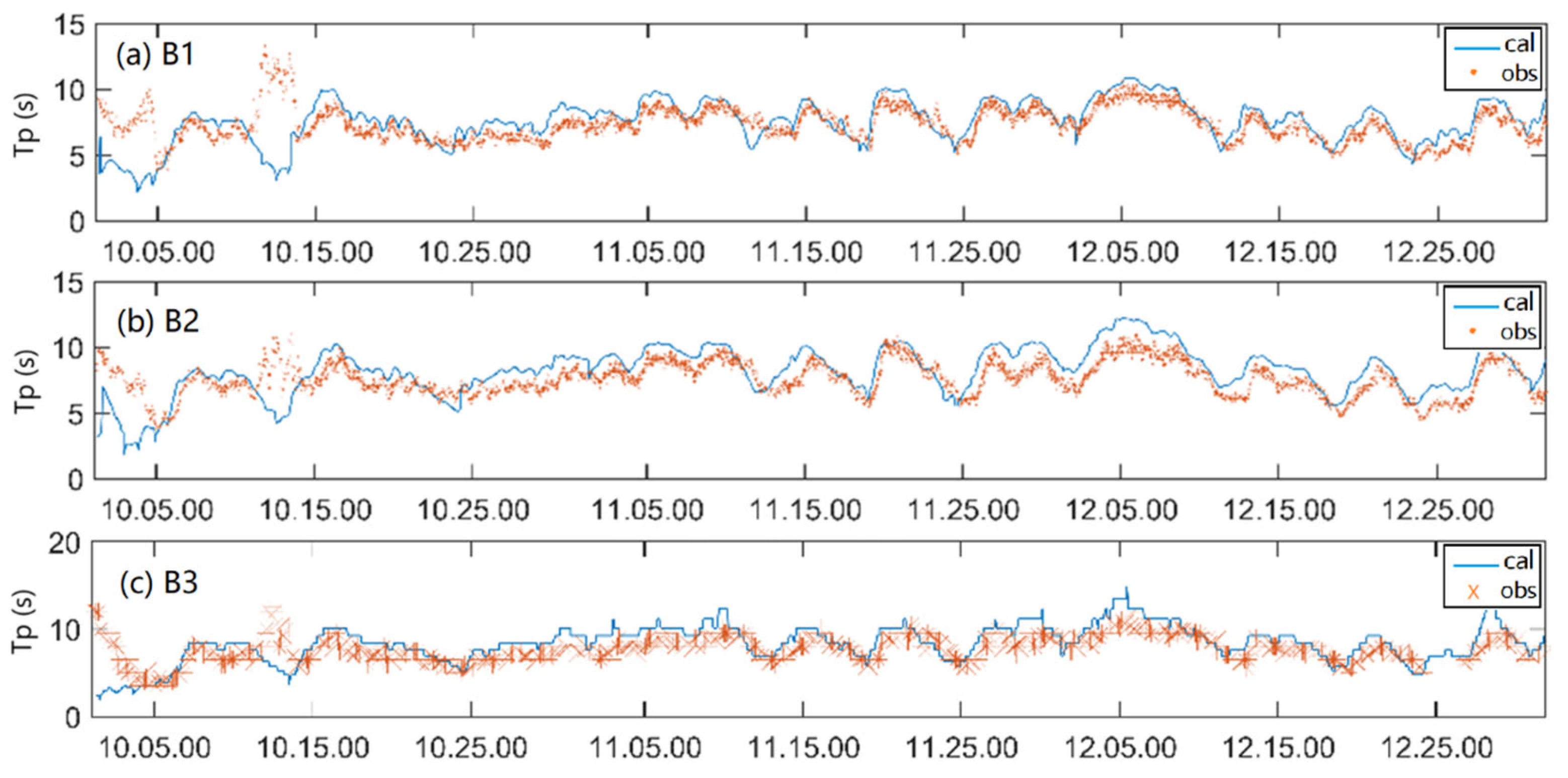
2.3. Wave Model Validation

Figure 2 presents comparisons of the observed and simulated $H_s$ at buoys B1, B2 and B3 (Figure 1) conducted between October and December 2019. Buoys B1 and B2 are located in the deep water of the SCS, while buoy B3 is located in the very shallow water of eastern Hainan Island. Both the observed and simulated $H_s$ values at these three buoy stations show obvious fluctuation during October and December 2019. The maximum observed $H_s$ values at buoys B1, B2 and B3 are about 6.5 m, 6.8 m and 2.5 m, respectively. The root mean square errors (RMSEs) at these three buoy stations are calculated to quantify model performance. The simulated $H_s$ values have RMSEs of 0.53 m, 0.51 m and 0.38 m at buoys B1, B2 and B3, respectively. Figure 2 demonstrates that the northwestern SCS wave model reproduces well the temporal and spatial distribution of $H_s$ at these buoy stations.

Figure 3 presents time series of the observed and simulated $T_p$ at buoys B1, B2 and B3 between October and December 2019. The $T_p$ values in the northwestern SCS mainly range between 6 s and 10 s, with a mean value of about 8.5 s at these three buoy stations. Figure 3 shows that the simulated $T_p$ values vary similarly with the observations at these buoy stations.

3. Method

The long-term joint distribution of sea states in the northwestern SCS is estimated, and this distribution is used to construct an environmental contour with a return period of 1, 5, 10, 25, 50 and 100 years in this study. The joint distribution of $H_s$ and $T_p$ is established using a conditional modeling approach. Firstly, the independent univariate distribution of $H_s$ needs to be created. Then, the dependent univariate distribution of $T_p$ is created and its dependency on $H_s$ is defined. Lastly, the environmental contours under various return periods are created using an inverse first-order reliability method (IFORM) [15]. The extreme sea states with a given return period will be defined according to the environmental contours.

3.1. Univariate Distribution Methods

A number of probability density functions (PDFs) have been proposed to describe the distributional forms of sea states [16]. Among these, four kinds of univariate distributions, namely, Normal, Lognormal, Gamma and three-parameter (3P) Weibull distributions, are commonly used to fit the probability distributions of $H_s$ and $T_p$ [17,18]. Their PDFs are described as follows:

Normal distribution:

$$f\left(x\right)={\displaystyle \frac{1}{\sqrt{2\pi }{\sigma }_s}}\exp \left\{-{\displaystyle \frac{{\left[x-\mu \right]}^2}{2{\sigma }_s^2}}\right\}, x>0$$

(1)

Lognormal distribution:

$$f_L\left(x\right)={\displaystyle \frac{1}{\sqrt{2\pi }{\sigma }_{s}x}}\exp \left\{-{\displaystyle \frac{{\left[\log x-\mu \right]}^2}{2{\sigma }_s^2}}\right\}, x>0$$

(2)

where $\mu$ and ${\sigma }_s$ are the mean parameter and standard deviation of the corresponding normal distribution, respectively.

Gamma distribution:

$$f\left(x\right)={\displaystyle \frac{1}{{\lambda }^k\mathsf{\Gamma }\left(k\right)}}{x}^{\left(k-1\right)}\exp \left(-{\displaystyle \frac{x}{\lambda }}\right)$$

(3)

where $\lambda ,k$ are the scale and shape parameters, respectively.

Three-parameter Weibull distribution:

$$f_w\left(x\right)={\displaystyle \frac{\beta }{\alpha }}{\left({\displaystyle \frac{x-\gamma }{\alpha }}\right)}^{\beta -1}\exp \left[-{\left({\displaystyle \frac{x-\gamma }{\alpha }}\right)}^{\beta }\right],x\ge \gamma$$

(4)

where $\alpha ,\beta ,\gamma$ are the scale, shape and location parameters of the three-parameter Weibull distribution, respectively.

3.2. Dependence Functions

The dependency of the conditional univariate distribution is described with dependence functions for the distribution’s parameters ($\mu \mathrm{a}\mathrm{n}\mathrm{d} \sigma$). Six dependence functions [19], namely, power3, exp3, insquare2, asymdecrease3, logistics4 and alpha3, used in the conditional distribution of $T_p$, which is dependent on $H_s$, are described in

Table 1. Dependence functions used in the conditional distribution.

Parametric Scheme	Dependence Function
$\mu$-power3	$\begin{array}{c}f\left(x\right)=a+b\ast x^c\end{array}$
$\sigma$-exp3	$\begin{array}{c}f\left(x\right)=a+b\ast e^{c\ast x}\end{array}$
$\mu$-insquare2	$\begin{array}{c}f\left(x\right)=\ln \left[a+b\ast \sqrt{\left(x/9.81\right)}\right]\end{array}$
$\sigma$-asymdecrease3	$\begin{array}{c}f\left(x\right)=a+b/\left(1+c\ast x\right)\end{array}$
$\mu$-logistics4	$\begin{array}{c}f\left(x\right)=a+b/\left[1+e^{-1\ast \left|c\right|\ast \left(x-d\right)}\right]\end{array}$
$\sigma$-alpha3	$\begin{array}{c}f\left(x\right)=\left(a+b\ast x^c\right)/{2.0445}^{1/logistics4\left(x,c_1,c_2,c_3,c_4\right)}\end{array}$

.

3.3. Bivariate Distribution Methods

The bivariate distribution model of $H_s$ and $T_p$, which is based on the total probability theorem, has been used previously by Lucas and Guedes Soares (2015) [17] and Huang and Dong (2020) [20]:

$$f\left(H_s,T_p\right)=f\left(H_s\right)\times f\left(T_p|H_s\right)$$

(5)

where $f\left(H_s,T_p\right)$ is the JPD function of $H_s$ and $T_p$, $f\left(H_s\right)$ is the marginal probability density function of $H_s$, and $f\left(T_p|H_s\right)$ is the conditional probability density function of $T_p$ dependent on $H_s$. $f\left(H_s\right)$ is described using the univariate distribution method introduced in Section 3.1. The distribution’s parameters in $f\left(T_p|H_s\right)$ are defined by the dependence functions in Section 3.2.

4. Results

A 42-year one-hourly sea state dataset has been obtained from the extensively validated SCS wave model which was run from 1 January 1979 to 31 December 2020. Figure 4 provides a description of $H_s$ and $T_p$ at station CZ. The largest and mean $H_s$ values are approximately 11.2 m and 1.5 m, and 24% of values are greater than 2 m. The vast majority of the sea states have $T_p$ values varying between 5 s and 10 s, with the longest $T_p$ being approximately 14.8 s.

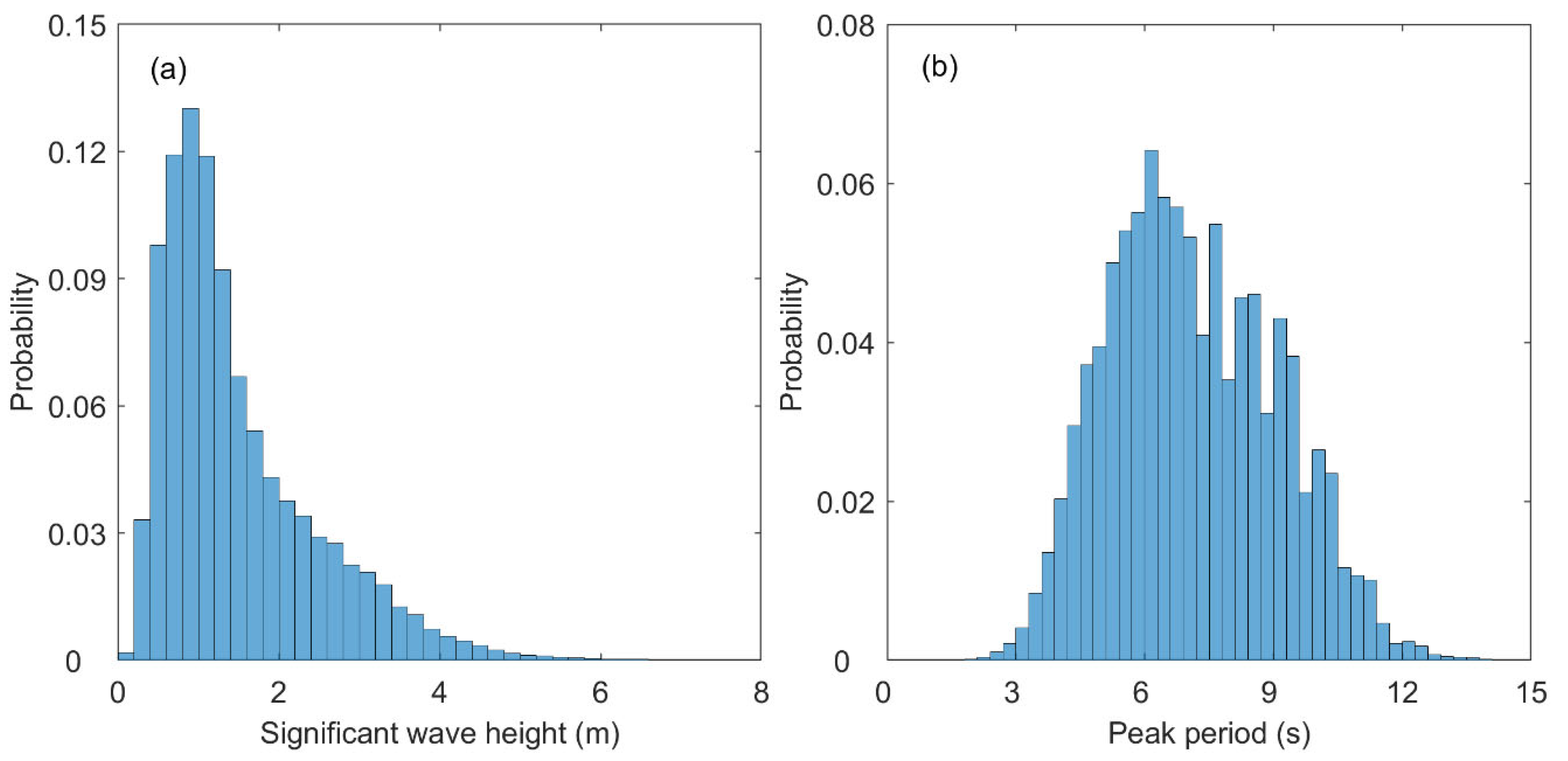
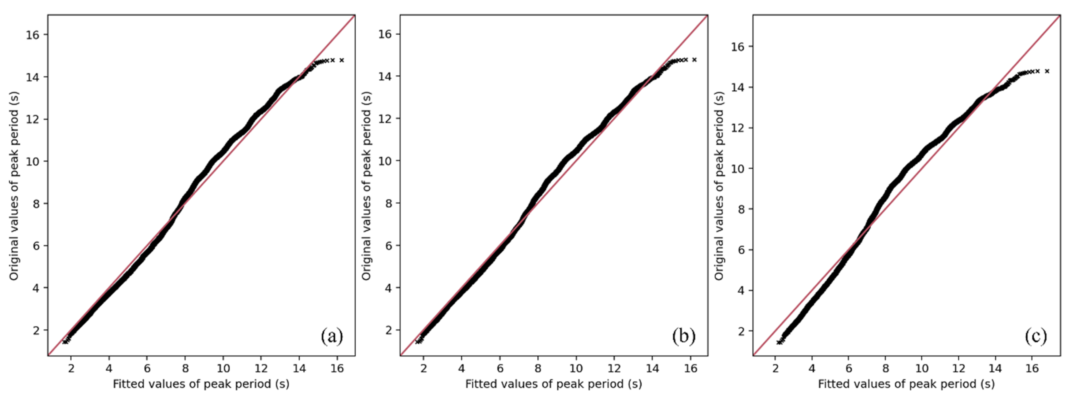
4.1. Marginal Distributions of $H_s$

The marginal independent distribution of $H_s$ at station CZ is fitted using four univariate distribution methods including Normal, Lognormal, Gamma and 3P Weibull distributions. The parameters in these univariate distribution functions can be calculated by the least squares method. Figure 5 presents comparisons of the original and fitted values of $H_s$ at station CZ. For the Normal distribution, the fitted values of $H_s$ match relatively well between 1.0 m and 2.5 m, though larger and smaller $H_s$ values are underestimated. For the Lognormal distribution, the fitted values of $H_s$ agree well with the original data for $H_s$ values smaller than 4.5 m. The Lognormal distribution overpredicts larger $H_s$ values, as the fitted values are almost twice the original value of 10 m. For the Gamma distribution, the fitted values are of good quality for smaller $H_s$ values < 5.0 m, while the distribution overestimates larger $H_s$ values. The 3P Weibull distribution performs better than the other three univariate distribution methods. The fitted values obtained using the 3P Weibull distribution agree well with the original data; only $H_s$ values between 6.5 m and 10.5 m tend to be slightly underestimated. As a result of this comparison, $H_s$ at station CZ is found to be suitable for the 3P Weibull distribution, which is advocated by Mathiesen and Bitner-Gregersen [21].

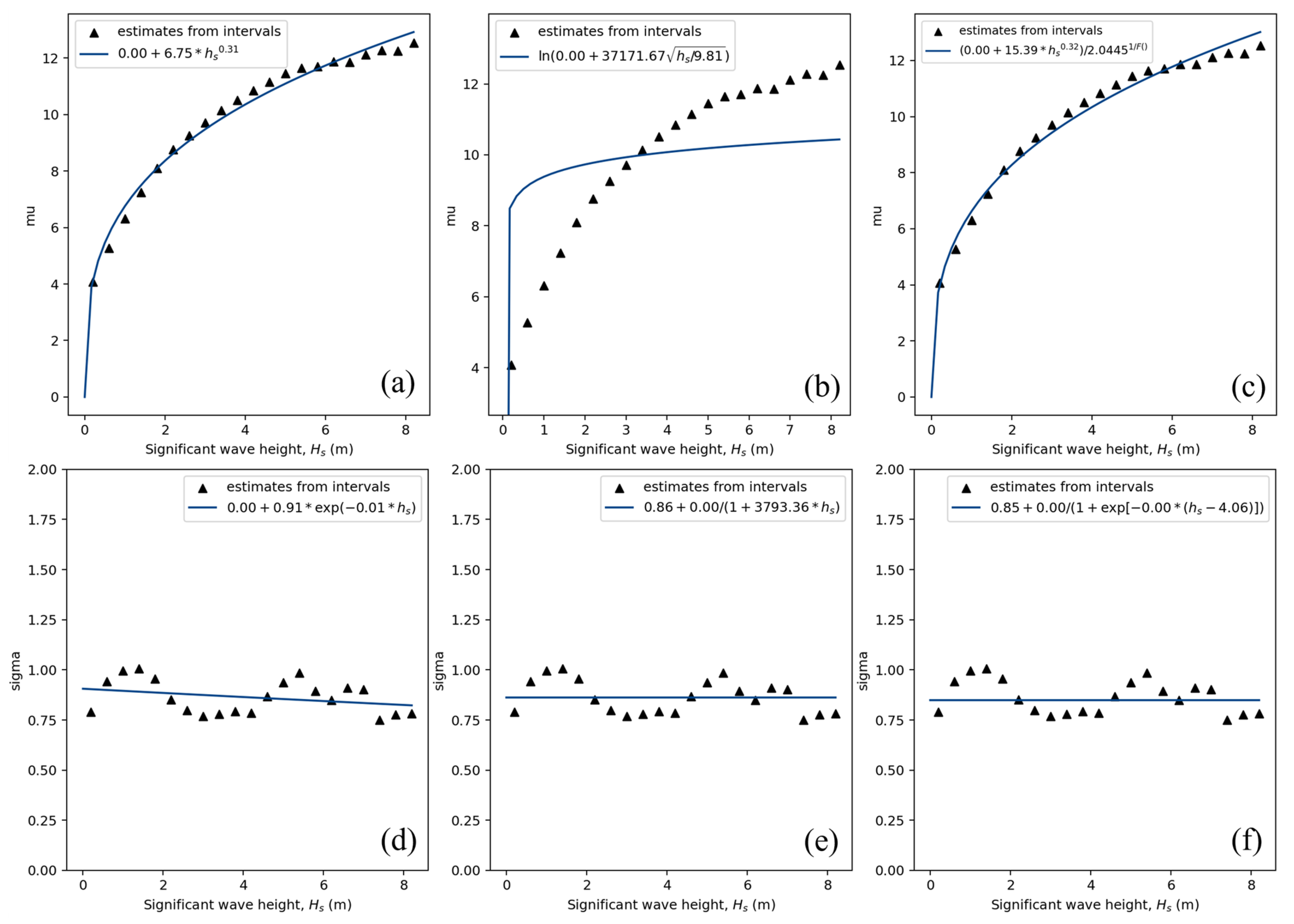
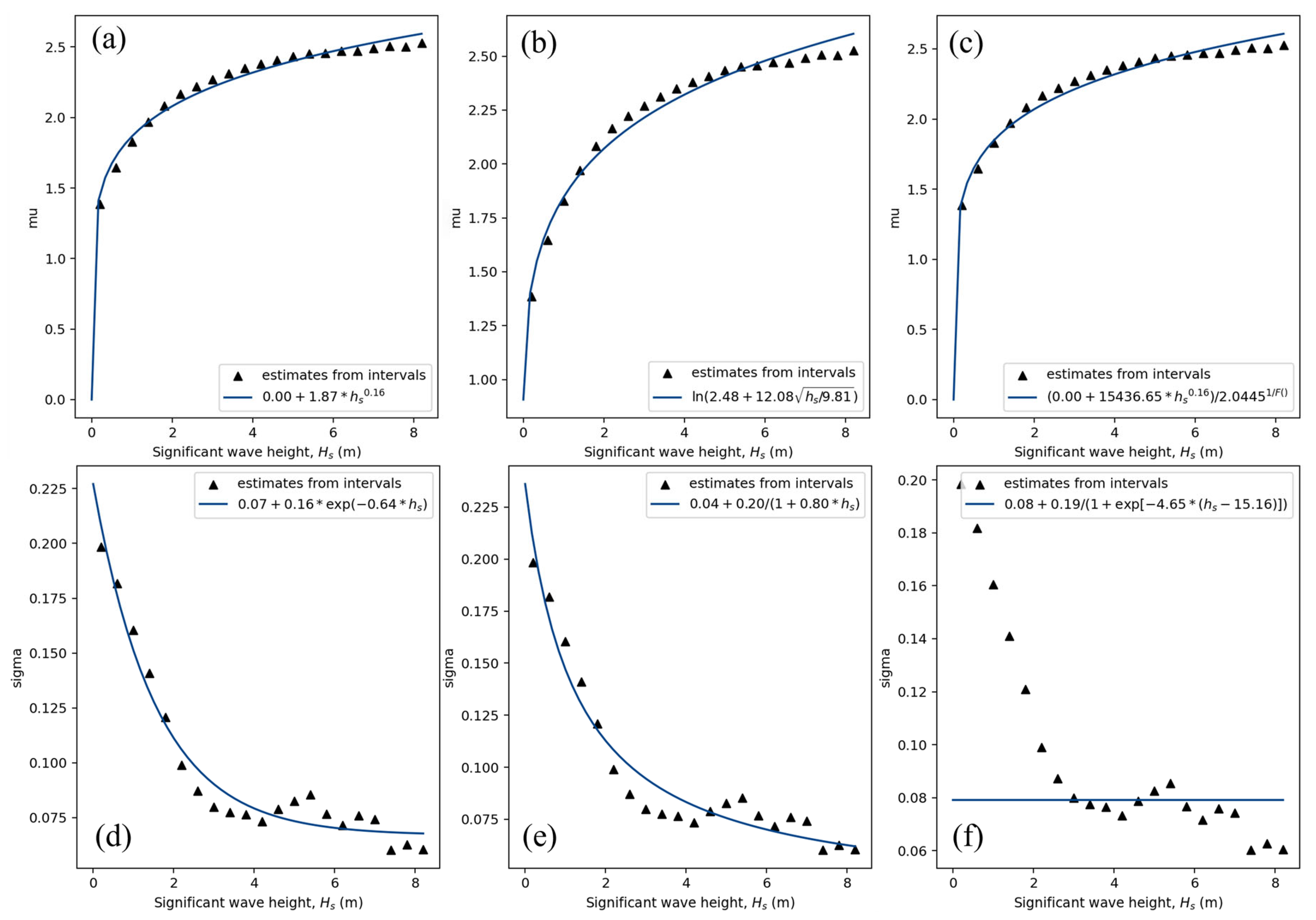
4.2. Dependence Functions and Conditional Distributions of $T_p$

In this study, the conditional modeling approach was used to construct a bivariate distribution as a product of the marginal distribution for $H_s$ and the conditional distribution for $T_p$. We used Normal and Lognormal distributions to create the conditional distribution for $T_p$, in which the parameters were calculated using the dependence functions described in Section 3.2.

Figure 6 presents the estimation of dependence functions ($\mu$ and $\sigma$) in the Normal distribution of $T_p$ dependent on the 3P Weibull distribution of $H_s$. The mean parameter $\mu$ and standard deviation $\sigma$ of the corresponding normal distribution use power3, insquare2, alpha3 and exp3, asymdecrease3, logistics4, respectively. The power3 and alpha3 functions fit the mean parameter $\mu$ well, while the insquare2 function shows worse performance. The exp3, asymdecrease3 and logistics4 functions have a similar ability to fit the standard deviation $\sigma$ in dependence functions for $T_p$. The estimations of $\sigma$ values show fluctuation depending on $H_s$. For the exp3 dependence function, the fitted $\sigma$ value is 0.91 when $H_s$ is 0 m, and the fitted $\sigma$ value decreases slightly with the increase in $H_s$. The asymdecrease3 and logistics4 functions give constant $\sigma$ values of 0.86 and 0.85, respectively.

The estimation of the Normal distribution for $T_p$ at station CZ using various dependence functions is conducted by comparing the fitted and original values of $T_p$ (Figure 7). When $\mu$ and $\sigma$ in Normal distribution use power3, exp3 and alpha3, logistics4 functions, the Normal distribution underestimates smaller $T_p$ values < 3 s and fits well for other $T_p$ values. These two Normal distributions perform better than the Normal distribution using insquare2 for $\mu$ and asymdecrease3 for $\sigma$, which overestimates most values of $T_p<12 \mathrm{s}$ and underestimates higher values of $T_p>12 \mathrm{s}$.

Figure 8 presents the estimation of dependence functions ($\mu$ and $\sigma$) in the Lognormal distribution of $T_p$ which is dependent on the 3P Weibull distribution of $H_s$. The mean parameter $\mu$ uses power3, insquare2 and alpha3 functions, respectively. The standard deviation $\sigma$ uses exp3, asymdecrease3 and logistics4 functions, respectively. The estimated $\mu$ values depending on $H_s$ show a parabolic growth pattern. The mean parameter $\mu$ is about 1.4 for the smallest $H_s$ and about 2.5 for an $H_s$ of 8.2 m. The power3, insquare2 and alpha3 functions have a similar ability to fit $\mu$ values, while smaller $\mu$ values are better fitted than larger $\mu$ values. The estimated $\sigma$ values depending on $H_s$ show a parabolic decrease pattern; $\sigma$ equals 0.2 for the smallest $H_s$ and about 0.07 for an $H_s$ of 8.2 m. The exp3 and asymdecrease3 functions give a similar parabolic distribution to the estimated $\sigma$ values and perform better than the logistics4 function. The $\sigma$ values calculated by the logistics4 function stay at 0.08 with negligible changes across various $H_s$ values.

The dependence functions of $\mu$ and $\sigma$ shown in Figure 8 are used to form the conditional distribution of $T_p$ using the Lognormal distribution method at station CZ. The fitted and original $T_p$ values are compared to assess the performance of the various dependence functions (Figure 9). The Lognormal distributions using the power3 and insquare2 functions for $\mu$ and the exp3 and asymdecrease3 functions for $\sigma$ perform well in producing $T_p$ values smaller than 8.0 s, while the fitted $T_p$ values from the Lognormal distribution using alpha3 and logistics4 are larger than the original values of $T_p$ smaller than 6.0 s. All three kinds of Lognormal distribution slightly underestimate $T_p$ values between 8.0 s and 13.0 s and overestimate $T_p$ values higher than 13.5 s.

By comprehensively comparing the performances of dependence functions for $\mu$, $\sigma$ and $T_p$, we can conclude that these three kinds of dependence functions show significant differences in fitting the mean parameter $\mu$ and standard deviation $\sigma$. The combination of power3 for $\mu$ and exp3 for $\sigma$ fits better than the other two combinations. The Lognormal distribution method performs better than the Normal distribution method in calculating $T_p$.

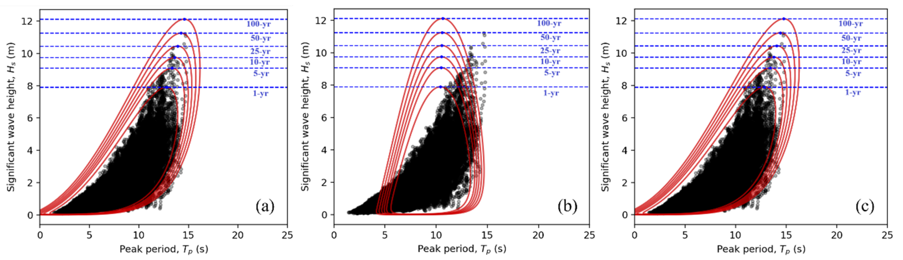
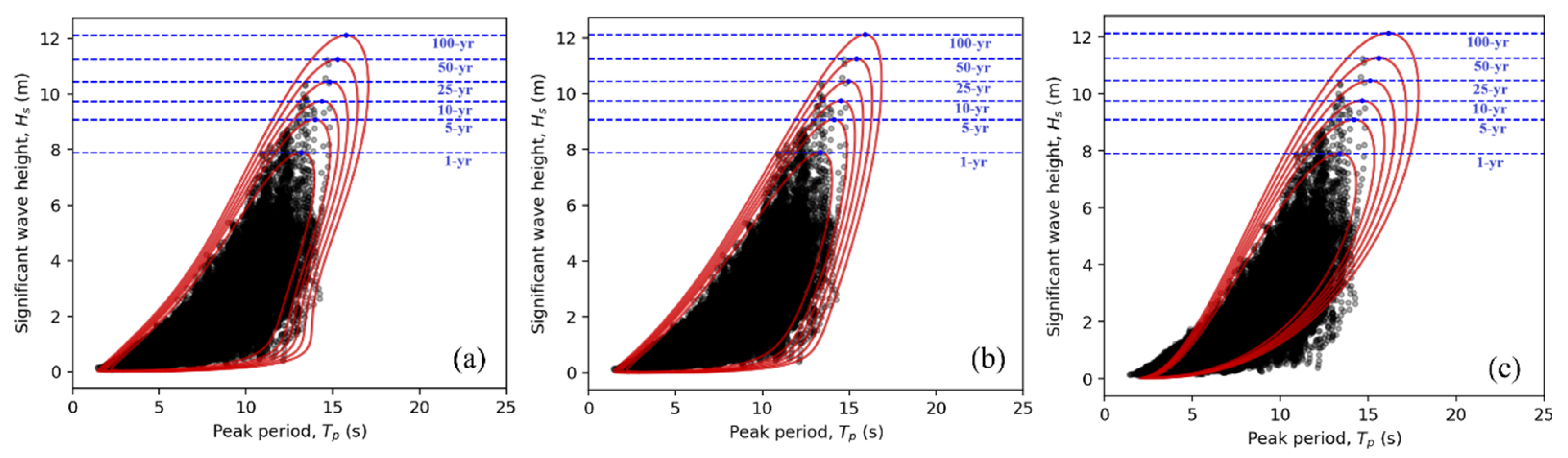
4.3. Environmental Contours and Extreme Sea States

The joint distributions of $H_s$ and $T_p$ are generated by using the global hierarchical probabilistic model, which combines the distributions and dependencies of $H_s$ and $T_p$, proposed by Haselsteiner et al. [22]. The factorization describes a hierarchy where a random variable with index i can only depend upon random variables with indices less than i. The environmental contour method is an effective method to prove efficiency in approximating the long-term extreme response [23]. These environmental contours are traditionally obtained by the inverse first-order reliability method (IFORM) [15] after defining the contour’s exceedance probability ($\alpha$):

$$\alpha =t_S/t_R$$

(6)

where $t_R$ is the return period; we chose return periods of 1, 5, 10, 25, 50 and 100 years. $t_S$ is the sea state duration, which is 1 h in this study.

The environmental contours derived by the joint distribution of $H_s$ using the 3P Weibull distribution and $T_p$ using the Normal distribution at station CZ are shown in Figure 10. Six levels of return periods are combined and plotted in the figures. The environmental contours using the combination of power3 and exp3 as dependence functions show a similar distribution shape to the original datasets, which are almost enveloped by the 50-year and 100-year contours. This joint distribution model slightly underestimates $T_p$ values for lower $H_s$ values. The environmental contours derived by the joint distribution model using insquare2 and asymdecrease3 as dependence functions provide completely different shapes, which are symmetrically distributed along $T_p=10.5 \mathrm{s}$. The data points with a lower $H_s$ and shorter $T_p$ and a higher $H_s$ and longer $T_p$ fall outside all the environmental contours. By contrast, the joint distribution model using alpha3 and logistics4 as dependence functions provides similar environmental contours to the first joint distribution model.

Figure 11 presents the environmental contours derived by the joint distribution of $H_s$ using the 3P Weibull distribution and $T_p$ using the Lognormal distribution at station CZ. The first joint distribution model using power3 and exp3 in the conditional Lognormal distribution provides reasonable estimates of the environmental contours. The lower $H_s$ and longer $T_p$ data points are enveloped inside the environmental contours. The environmental contours from the second joint distribution model using insquare2 and asymdecrease3 as dependence functions show a similar shape to the above results, except that the range of $T_p$ values for higher $H_s$ values is slightly narrower than in the previous contours. The environmental contours from the third joint distribution model using alpha3 and logistics4 as dependence functions show significant differences compared to the first two models, especially for lower $H_s$ and fringe $T_p$ values, for which the data points fall outside the environmental contours. In addition, all three types of joint distribution models overpredict higher $T_p$ values, which is also shown in Figure 9.

The extreme sea states with given return periods can be calculated depending on the environmental contours. We obtain extreme $H_s$ values by making tangents to the environmental contours and take the corresponding $T_p$ values. The extreme sea states at station CZ with return periods of 1, 5, 10, 25, 50 and 100 years using Normal and Lognormal conditional distributions for $T_p$ are listed in

Table 2. Extreme sea states at station CZ with return periods of 1, 5, 10, 25, 50 and 100 years using Normal conditional distribution for $T_p$.

Return Period (Year)	Power3/Exp3		Insquare2/Asymdecrease3		Logistics4/Alpha3
	Hs (m)	Tp (s)	Hs (m)	Tp (s)	Hs (m)	Tp (s)
1	7.9	12.8	7.9	10.4	7.9	12.9
5	9.1	13.3	9.1	10.5	9.1	13.5
10	9.8	13.6	9.8	10.5	9.8	13.8
25	10.4	13.9	10.4	10.6	10.4	14.1
50	11.2	14.2	11.2	10.6	11.2	14.4
100	12.1	14.6	12.1	10.6	12.1	14.8

and

Table 3. Extreme sea states at station CZ with return periods of 1, 5, 10, 25, 50 and 100 years using Lognormal conditional distribution for $T_p$.

Return Period (Year)	Power3/Exp3		Insquare2/Asymdecrease3		Logistics4/Alpha3
	Hs (m)	Tp (s)	Hs (m)	Tp (s)	Hs (m)	Tp (s)
1	7.9	13.2	7.9	13.3	7.9	13.4
5	9.1	13.9	9.1	14.1	9.1	14.2
10	9.8	14.4	9.8	14.5	9.8	14.6
25	10.4	14.8	10.4	14.9	10.4	15.1
50	11.2	15.3	11.2	15.4	11.2	15.6
100	12.1	15.8	12.1	15.9	12.1	16.1

. All these extreme $H_s$ values are obtained from the 3P Weibull marginal distribution; therefore, the extreme sea states show unique $H_s$ values of 7.9, 9.1, 9.8, 10.4, 11.2 and 12.1 m for return periods of 1, 5, 10, 25, 50 and 100 years, respectively. The $T_p$ values corresponding to the extreme $H_s$ values are 12.8, 13.3, 13.6, 13.9, 14.2 and 14.6 s with power3 and exp3 as dependence functions in the Normal distribution. As reported above, the $T_p$ value corresponding to an extreme $H_s$ value obtained from the Normal distribution using insquare2 and asymdecrease3 varies between 10.4 s and 10.6 s. For logistics4 and alpha3, $T_p$ is 0.2 s longer than the corresponding $T_p$ with power3 and exp3 as dependence functions.

The $T_p$ corresponding to the extreme $H_s$ derived by the Lognormal distribution is longer than that derived by the Normal distribution. For the Lognormal distribution using power3 and exp3, the $T_p$ values are 13.2, 13.9, 14.4, 14.8, 15.3 and 15.8 s for return periods of 1, 5, 10, 25, 50 and 100 years, respectively. When insquare2 and asymdecrease3 or logistics4 and alpha3 are used as dependence functions in the Lognormal distribution, the change in $T_p$ with power3 and exp3 is smaller than 0.3 s.

5. Conclusions

In this study, the joint distribution of significant wave heights and peak wave periods in the northwestern SCS was established using a dataset derived from an extensively validated wave model. To ensure that we had sufficiently long-term datasets to analyze extreme environmental parameters, an unstructured triangular mesh wave model covering the northwestern SCS was established based on the third-generation spectral wave model SWAN. This wave model has been extensively validated against quality-controlled field data and was run from 1979 to 2020 to generate one-hourly $H_s$ and $T_p$ measurements.

The joint distribution of $H_s$ and $T_p$ was established using a conditional modeling approach. For comparison, four probability density functions including Normal, Lognormal, Gamma and 3P Weibull distributions were adopted to construct the marginal independent distribution of $H_s$ at station CZ. As a result of this estimation between fitted and original values, the $H_s$ at station CZ is found to be suitable for the 3P Weibull distribution.

The dependence functions of the conditional univariate distribution are key parametric functions used to define the distribution of $T_p$. Three combinations of $\mu \mathrm{and} \sigma$, namely, power3 and exp3, insquare2 and asymdecrease3, and logistics4 and alpha3, were used to create Normal and Lognormal distributions for $T_p$. For the Normal distribution, the first and third combinations perform better than the second combination in fitting the estimated parametric values and original $T_p$. For the Lognormal distribution, the assessment of the fitted model shows that the first combination gives a reasonable description of the pattern of $T_p$.

Furthermore, the environmental contours derived by the IFORM were used to generate extreme sea states with return periods of 1, 5, 10, 25, 50 and 100 years. The results show that extreme $H_s$ is determined by the 3P Weibull distribution, with return values of 7.9, 9.1, 9.8, 10.4, 11.2 and 12.1 m for return periods of 1, 5, 10, 25, 50 and 100 years. The $T_p$ corresponding to an extreme $H_s$ varies with the dependence functions, and the $T_p$ values are 13.2, 13.9, 14.4, 14.8, 15.3 and 15.8 s for $\mu \mathrm{and} \sigma$ using power3 and exp3, which is the most reasonable combination of dependence functions.

The main focus of this study was the most suitable patterns of the marginal distribution of $H_s$ and the dependence functions of the conditional distribution of $T_p$ in the northwestern SCS. In future work, comparisons of extreme sea states derived from probability distributions for single metocean parameters and joint distributions need to be conducted. The applicability of the distributions established in this manuscript need to be checked using observational datasets for other regions.

References

1. Lee, U.J.; Cho, H.Y.; Lee, B.W.; Ko, D.H. Joint probability distribution of significant wave height and peak wave period using gaussian copula method. J. Coast. Res. 2023, 116, 96–100. [Google Scholar] [CrossRef]
2. Bitner-Gregersen, E.M. Joint probabilistic description for combined seas. In Proceedings of the International Conference on Offshore Mechanics and Arctic Engineering 2005 (OMAE2005), Volume 2: Safety and Reliability, Ocean Space Utilization, Ocean Engineering, Halkidiki, Greece, 12–17 June 2005. [Google Scholar]
3. Longuet-Higgins, M.S. On the joint distribution of the periods and amplitudes of sea waves. J. Geophys. Res. 1975, 80, 2688–2694. [Google Scholar] [CrossRef]
4. Longuet-Higgins, M.S. On the Joint Distribution of Wave Periods and Amplitudes in a Random Wave Field. Proc. R. Soc. Lond. A 1983, 389, 241–258. [Google Scholar] [CrossRef]
5. Sun, F. On the Joint Distribution of the Periods and Heights of Sea Waves. Acta Oceanol. Sin. 1987, 4, 503–509. Available online: http://www.en.cnki.com.cn/Article_en/CJFDTOTAL-SEAE198704001.htm (accessed on 10 March 2025).
6. Zheng, G.; Jiang, X.; Han, S. The Difference between the Joint Probability Distributions of Apparent Wave Heights and Periods and Individual Wave Heights and Periods. Acta Oceanol. Sin. 2004, 23, 399–406. [Google Scholar]
7. Stansell, P.; Wolfram, J.; Linfoot, B. Improved Joint Probability Distribution for Ocean Wave Heights and Periods. J. Fluid Mech. 2004, 503, 273–297. [Google Scholar] [CrossRef]
8. Zhang, H.D.; Guedes Soares, C. Engineering Modified Joint Distribution of Wave Heights and Periods. China Ocean Eng. 2016, 30, 359–374. [Google Scholar] [CrossRef]
9. James, J.P.; Panchang, V. Assessment of Joint Distributions of Wave Heights and Periods. Ocean Eng. 2024, 313, 119501. [Google Scholar] [CrossRef]
10. Prince-Wright, R. Maximum Likelihood Models of Joint Environmental Data for TLP Design. In Proceedings of the International Conference on Offshore Mechanics and Arctic Engineering, Copenhagen, Denmark, 18–22 June 1995. [Google Scholar]
11. Bitner-Gregersen, E.M.; Haver, S. Joint environmental model for reliability calculations. In Proceedings of the First International Offshore and Polar Engineering Conference, Edinburgh, UK, 11–16 August 1991. [Google Scholar]
12. Bitner-Gregersen, E.; Soares, C.G.; Machado, U.; Cavaco, P. Comparison of different approaches to joint environmental modelling. In Proceedings of the 17th International Conference on Offshore Mechanics and Arctic Engineering (OMAE 1998), Lisbon, Portugal, 5–9 July 1998. [Google Scholar]
13. Salvadori, G.; Durante, F.; Tomasicchio, G.R.; D’Alessandro, F. Practical Guidelines for the Multivariate Assessment of the Structural Risk in Coastal and Off-Shore Engineering. Coast. Eng. 2015, 95, 77–83. [Google Scholar] [CrossRef]
14. Allard, R.; Rogers, E.; Carroll, S.N. User’s Manual for the Simulating Waves Nearshore Model (SWAN); Storming Media: New York, NY, USA, 2002. [Google Scholar] [CrossRef]
15. Winterstein, S.R.; Ude, T.C.; Cornell, C.A.; Bjerager, P.; Haver, S. Environmental Parameters for Extreme Response: Inverse FORM with Omission Factors. In Proceedings of the ICOSSAR-93, Innsbruck, Austria, 9–13 August 1993. [Google Scholar]
16. Wu, Y.; Randell, D.; Christou, M.; Ewans, K.; Jonathan, P. On the Distribution of Wave Height in Shallow Water. Coast. Eng. 2016, 111, 39–49. [Google Scholar] [CrossRef]
17. Lucas, C.; Guedes Soares, C. Bivariate Distributions of Significant Wave Height and Mean Wave Period of Combined Sea States. Ocean Eng. 2015, 106, 341–353. [Google Scholar] [CrossRef]
18. Zhao, M.; Deng, X.; Wang, J. Description of the Joint Probability of Significant Wave Height and Mean Wave Period. JMSE 2022, 10, 1971. [Google Scholar] [CrossRef]
19. Bitner-Gregersen, E.M. Joint Met-Ocean Description for Design and Operations of Marine Structures. Appl. Ocean Res. 2015, 51, 279–292. [Google Scholar] [CrossRef]
20. Huang, W.; Dong, S. Joint Distribution of Significant Wave Height and Zero-up-Crossing Wave Period Using Mixture Copula Method. Ocean Eng. 2021, 219, 108305. [Google Scholar] [CrossRef]
21. Mathisen, J.; Bitner-Gregersen, E. Joint Distributions for Significant Wave Height and Wave Zero-up-Crossing Period. Appl. Ocean Res. 1990, 12, 93–103. [Google Scholar] [CrossRef]
22. Haselsteiner, A.F.; Sander, A.; Ohlendorf, J.H.; Thoben, K.D. Global Hierarchical Models for Wind and Wave Contours: Physical Interpretations of the Dependence Functions. In Proceedings of the 39th International Conference on Ocean, Offshore and Arctic Engineering (OMAE 2020), Online, 3–7 August 2020. [Google Scholar]
23. Chai, W.; Leira, B.J. Environmental Contours Based on Inverse SORM. Mar. Struct. 2018, 60, 34–51. [Google Scholar] [CrossRef]
Figure 1. Domain and bathymetry of the northwestern SCS wave model. Three pink triangles indicate positions of in situ observation stations.
Jmse 13 00570 g001
Figure 2. Time series of significant wave heights at B1, B2 and B3 stations derived from observations and simulations between October and December 2019.
Jmse 13 00570 g002
Figure 3. Time series of peak wave periods at B1, B2 and B3 stations derived from observations and simulations between October and December 2019.
Jmse 13 00570 g003
Figure 4. Distribution of (a) significant wave height and (b) peak wave period at station CZ.
Jmse 13 00570 g004
Figure 5. Comparison of original and fitted values of significant wave height at station CZ. (a): Normal, (b): Lognormal, (c): Gamma and (d): 3P Weibull distribution methods.
Jmse 13 00570 g005
Figure 6. Estimation of dependence functions ( μ and σ ) in conditional Normal distribution of T p dependent on 3P Weibull distribution of Hs. (a): μ -power3; (b): μ -insquare2; and (c): μ -alpha3 and (d): σ -exp3; (e): σ -asymdecrease3; and (f): σ -logistics4.
Jmse 13 00570 g006
Figure 7. Conditional distribution of peak wave period at station CZ using Normal distribution method with various dependence functions. (a): μ -power3 and σ -exp3; (b): μ -insquare2 and σ -asymdecrease3; (c): μ -alpha3 and σ -logistics4.
Jmse 13 00570 g007
Figure 8. Estimation of dependence functions ( μ and σ ) in conditional Lognormal distribution of T p dependent on 3P Weibull distribution of H s . (a): μ -power3; (b): μ -insquare2; (c): μ -alpha3; (d): σ -exp3; (e): σ -asymdecrease3; (f): σ -logistics4.
Jmse 13 00570 g008
Figure 9. Conditional distribution of peak wave period at station CZ using Lognormal distribution method with various dependence functions. (a): μ -power3 and σ -exp3; (b): μ -insquare2 and σ -asymdecrease3; (c): μ -alpha3 and σ -logistics4.
Jmse 13 00570 g009
Figure 10. Environmental contours for joint distribution of H s using 3P Weibull distribution and T p using Normal distribution with various dependence functions. (a): μ -power3 and σ -exp3; (b): μ -insquare2 and σ -asymdecrease3; (c): μ -alpha3 and σ -logistics4.
Jmse 13 00570 g010
Figure 11. Environmental contours for joint distribution of H s using 3P Weibull distribution and T p using Lognormal distribution with various dependence functions. (a): μ -power3 and σ -exp3; (b): μ -insquare2 and σ -asymdecrease3; (c): μ -alpha3 and σ -logistics4.
Jmse 13 00570 g011