Abstract
Offshore wind turbines are subjected to long-term cyclic loads, and the seabed materials surrounding the foundation are susceptible to failure, which affects the safe construction and normal operation of offshore wind turbines. The existing studies of the cyclic mechanical properties of submarine soils focus on the accumulation strain and liquefaction, and few targeted studies are conducted on the hysteresis loop under cyclic loads. Therefore, 78 representative submarine soil samples from four offshore wind farms are tested in the study, and the cyclic behaviors under different confining pressures and CSR are investigated. The experiments reveal two unique development modes and specify the critical CSR of five submarine soil martials under different testing conductions. Based on the dynamic triaxial test results, the machine learning-based partition models for cyclic development mode were established, and the discrimination accuracy of the hysteresis loop were discussed. This study found that the RF model has a better generalization ability and higher accuracy than the GBDT model in discriminating the hysteresis loop of submarine soil, the RF model has achieved a prediction accuracy of 0.96 and a recall of 0.95 on the test dataset, which provides an important theoretical basis and technical support for the design and construction of offshore wind turbines.
1. Introduction
As a crucial part of the new energy sector, offshore wind power has become a trendy and much-discussed topic [1,2]. As per the comprehensive data sourced from the Global Wind Energy Council, as cited in reference [3], by the terminal point of the year 2023, the aggregate cumulative installed capacity of the global offshore wind power sector had reached a significant milestone of 75.2 GW, underscoring the notable growth and development within the realm of offshore wind energy infrastructure on a global scale. At present, the cumulative installed capacity of China’s offshore wind farms has reached 39.1 gigawatts, ranking first in the world. Basic safety is very important in the construction and commissioning of offshore wind turbines. The related construction costs account for about 30% of the total investment of offshore wind farms [4], which is one of the key factors affecting the economic feasibility of the project. As the construction material of offshore wind power foundation, the accurate disclosure of mechanical properties of marine soil is very important to ensure the safety and stability of the foundation structure [5]. Through in-depth study of the mechanical properties of marine soil, it can not only optimize the foundation design and reduce the construction risk, but also significantly reduce the maintenance and replacement costs caused by foundation failure, thereby improving the overall economic benefits of the project. In addition, with the continuous expansion of offshore wind power, the improvement of basic design and construction technology will further promote the industry to reduce costs and increase efficiency and provide stronger support for global energy transformation.
Offshore wind turbines are subjected to long-term cyclic loads, including wind, wave, and flow forces, and the seabed materials surrounding the foundation are susceptible to failure under these cyclic loads [6,7]. The cyclic behaviors of submarine soil have been systematically researched, and many classic and representative conclusions are obtained, i.e., the strain accumulation law [8,9], the stiffness attenuation law [10,11,12], the pore water pressure change [13,14], and cyclic failure criterion [15,16]. When subjected to cyclic loads, the stress–strain curve of the soil materials manifests as the hysteresis loop [17]. In addition to the several parameter indicators above, the hysteresis loop can represent cyclic mechanical properties of soil materials [18]. For example, Dai et al. [19] quantified the morphological characteristics of the hysteresis loop of soft clay and put forward the energy dissipation-based cyclic failure criterion, which provides a good reference for the related studies. Doygun et al. [20] studied the morphological characteristics of the hysteresis loop of five kinds of sand soils with high strain and analyzed the change law of the axial strain and consumption energy under one cycle cyclic load. As an important index of soil cyclic behaviors, the in-depth analysis of the hysteretic curve is of great significance to reveal the deformation law, stiffness change, and energy dissipation capacity. Under cyclic loading, the failure criterion of marine soil is not yet clear. The current research mostly uses strain development as a cyclic failure criterion, but this criterion ignores the effects of other cyclic characteristics such as pore pressure growth and stiffness weakening. Therefore, it is necessary to combine the various cyclic characteristics of soil to further improve the cyclic failure criterion of marine soil. And China’s marine soil is widely distributed, and the soil properties in different regions are quite different. In the current research, the marine soil samples used for the test are often taken from specific areas, and the diversity and representativeness of the samples are limited. It is difficult to cover all types of marine soil, which limits the universality of the research results.
Due to the complexity of the actual marine environment and the limitations of experimental verification, it is difficult to find suitable field data or experimental data to fully and effectively verify the numerical simulation results. This makes the application of numerical simulation in the study of the hysteresis curve of marine soil restricted, and the credibility of the simulation results needs to be further improved. In recent years, machine learning algorithms, such as artificial neural networks, support vector machines, and XGBoost, have rapidly advanced and found widespread applications in the field of civil engineering [21,22]. These methods have been employed to predict the dynamic elastic modulus of soils [23], the shear strength of subgrade soils [24], rock strength prediction [25], rock type classification [26], and the compressive strength of 3D-printed fiber-reinforced concrete [27]. There have also been numerous applications in the prediction of submarine soil properties. For example, Zhang et al. [28] developed a predictive model for the cumulative strain of marine soils using particle swarm optimization and random forest algorithms, and further analyzed the model using SHAP methods. Wang et al. [29] treated marine soft soils with solid waste materials and, using experimental data and collected field data, established a strength prediction model for soil stabilization based on the BP neural network algorithm. These studies demonstrate that machine learning-based algorithms can generate accurate soil property prediction models, effectively reducing the workload of laboratory experiments and construction sites. Therefore, it is essential to develop an intelligent method for the classification of hysteresis curves based on machine learning algorithms.
In this study, 78 representative submarine soil samples were collected from four offshore wind farms, and their cyclic behaviors under different confining pressures and CSR were investigated. Through critial CSR, the machine learning-based partition models for cyclic development mode are established, and the research results provide an important theoretical basis and technical support for the design and construction of offshore wind turbines.
2. Tests and Samples
2.1. Submarine Soils from Offshore Wind Farms
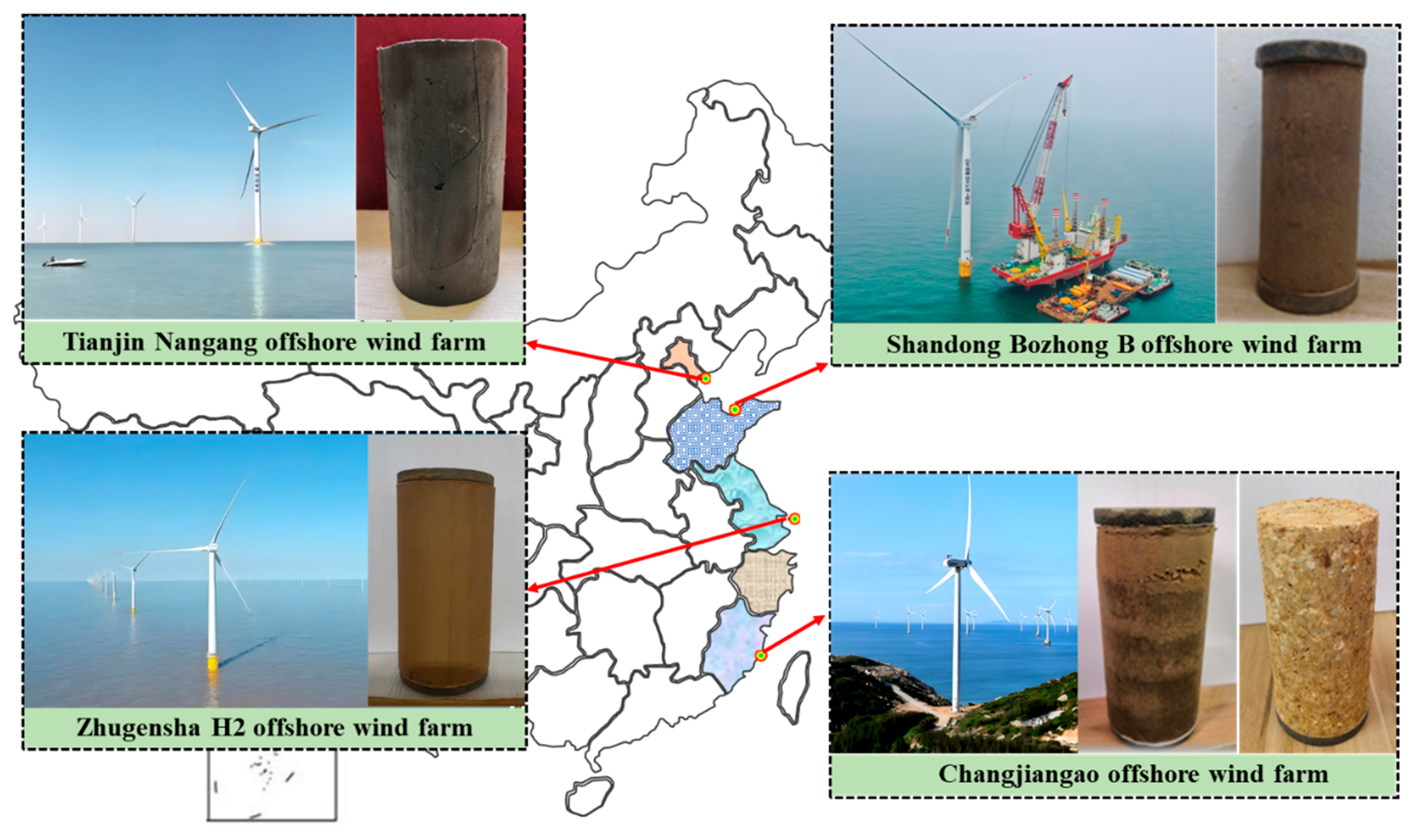
The total offshore wind energy capacity in China is approximately 750 GW, and the offshore wind power sector has significant development potential. The seas surrounding China encompass a vast area and extend across a wide range of north–south latitudes, which are categorized into the Bohai Sea, Yellow Sea, East China Sea, and South China Sea from north to south. The types and characteristics of seabed strata in offshore wind farms differ considerably across these various sea regions. In the Bohai Sea region, the seabed is predominantly composed of mucky clay and sandy clay. The Yellow Sea area primarily features sandy soil, while the East China Sea is characterized by thick layers of silt. The seabed in the Fujian and Guangdong regions are mainly composed of weathered granite. In the South China Sea, the seabed largely comprises calcareous sand and coral reef materials. The geological origins of these various seabed materials differ significantly, resulting in notable variations in their mechanical properties. In the study, 78 representative submarine rock and soil samples were collected from four offshore wind farms located in the Bohai Sea, Yellow Sea, and East China Sea. The tested soil samples included mucky clay, silty clay, silty soil, weathered residual soil, and completely weathered granite, as shown in Figure 1.

Figure 1.
Testing soil samples from four offshore wind turbines in China.
Mucky clay (MC) was collected from the Tianjin Nangang Offshore Wind Farm in the Bohai Sea, while silty clay (SC) was sourced from the Shandong Bozhong B Site Offshore Wind Farm, also in the Bohai Sea. Silty soil (SS) was obtained from the Zhugensha H2 Offshore Wind Farm in Nantong. Additionally, weathered residual soil (WRS) and completely weathered granite (CWG) were collected from the Pingtan Changjiangao Offshore Wind Farm in Fujian. The fundamental physical and mechanical properties of the five typical seabed soil materials from offshore wind farms are illustrated in Table 1.

Table 1.
Basic physical properties of five submarine soil martials.
2.2. Testing Instrument and Experimental Processes
The experimental apparatus employed in this study is the ELDyn standard dynamic triaxial test system (Figure 2), produced by GDS Instruments in the United Kingdom. This system consists of several key components, including a vertical loading system, a pressure chamber, a GDS control system, a back pressure controller, a confining pressure controller, and a data acquisition unit. Equipped with the proprietary GDSLab software (v2.5.0), the system is capable of applying a wide range of load magnitudes (0 to 5 kN) as well as static and dynamic loads at varying frequencies (0.1 to 5 Hz) to the soil specimens. Additionally, the apparatus is designed to precisely measure critical parameters such as pore water pressure, axial strain, axial stress, and other relevant mechanical properties of the soil samples during testing.
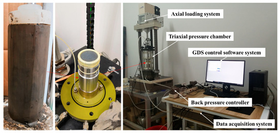
Figure 2.
Testing instrument and experimental processes.
According to the “Specification of Soil Test” (SL237-1999), the undisturbed soil samples collected in the offshore wind farms are firstly prepared in the standard cylindrical geotechnical samples measuring 50 mm in diameter and 100 mm in height. The samples must then be saturated and subjected to vacuum saturation for 24 h. Once prepared, the soil samples are placed in the testing apparatus, where consolidation and shear tests are conducted to complete the evaluation. In this study, the axial load applied is a sinusoidal cyclic load with a period of 3 s, and the load intensity is regulated by the cyclic stress ratio (CSR). which is defined as the ratio of the cyclic load amplitude () to confining pressure () imposed on soil testing samples. The confining pressure during the test is determined based on the specific gravity and burial depth of the soil samples. The testing procedures and schemes for the five soil masses are presented in Table 2.
Table 2.
Dynamic test schemes of five submarine soil martials.
3. Cyclic Failure Mode of Submarine Soil
3.1. Cyclic Behavior of Submarine Soil
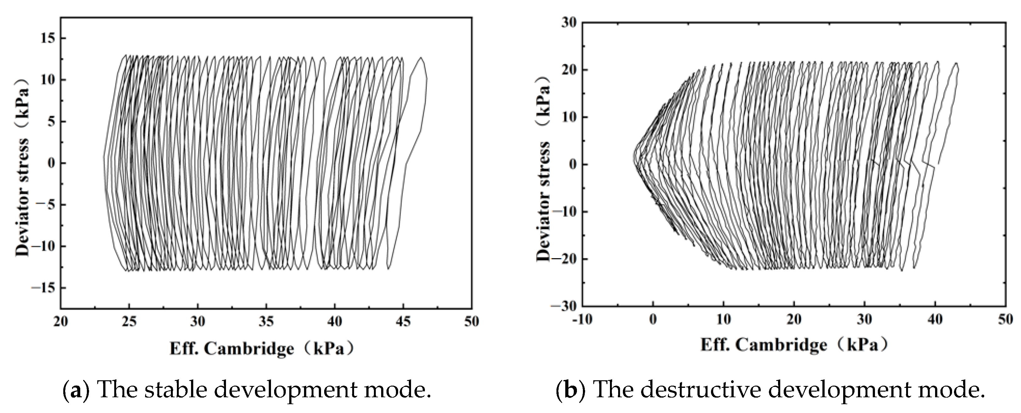
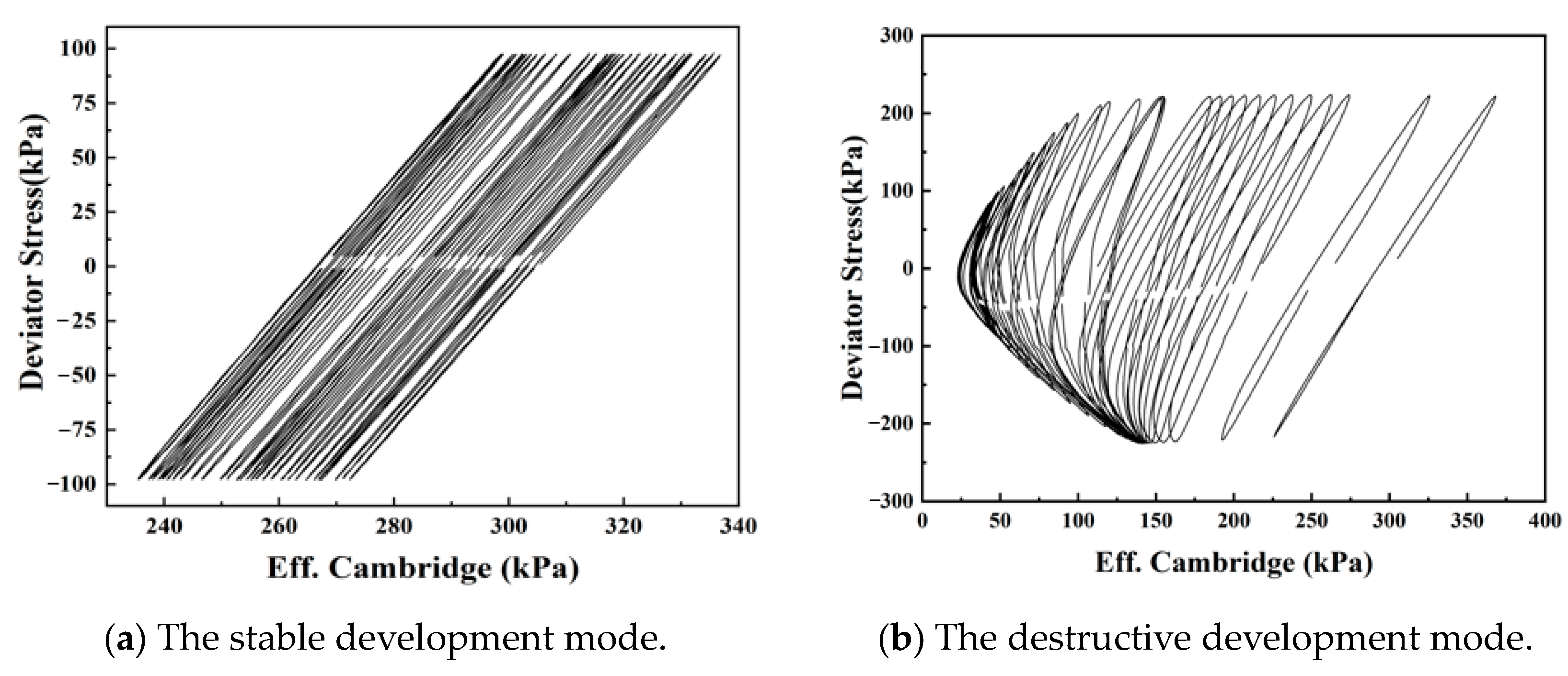
The cyclic behavior of submarine soils from offshore wind farms has been proved to exhibit distinctly different development modes under various cyclic loads. These modes can be categorized into two unique types: the stable development mode, which occurs under small cyclic loads, and the destructive development mode, which arises under large cyclic loads. The effective stress path serves as a case study to demonstrate the cyclic behavior of seabed soil in offshore wind farms subjected to various cyclic loading conditions, as shown in Figure 3, Figure 4, Figure 5 and Figure 6. Due to the continuous accumulation of pore water pressure in marine soil samples subjected to cyclic loading, the effective stress of the soil samples gradually decreases in accordance with the principle of effective stress. This phenomenon causes the effective stress path to continuously move towards the direction of decreasing average effective stress until it approaches the critical state line.
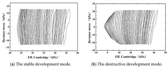
Figure 3.
The cyclic effective stress path of marine muck clay.
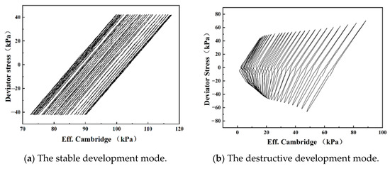
Figure 4.
The cyclic effective stress path of marine silt clay.
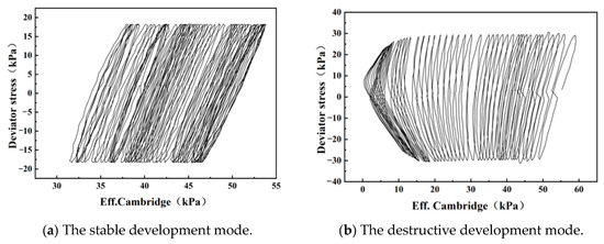
Figure 5.
The cyclic effective stress path of marine weathered residual soil.
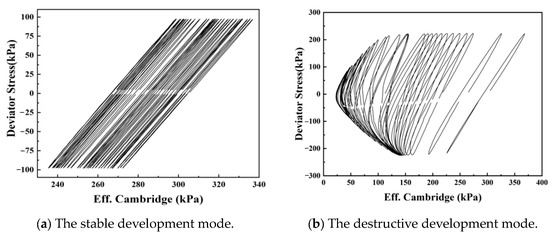
Figure 6.
The cyclic effective stress path of marine completely weathered granite.
Under low-intensity cyclic loads, the disturbance to the testing soil sample is minimal. The pore water pressure within the soil body increases slowly, while the effective stress decreases gradually. Consequently, the effective stress path shifts gradually from right to left. Nevertheless, throughout the progression along the effective stress path, the trajectory of stress exhibits consistency, characterized by the absence of substantial alterations in its slope, amplitude, and morphology, thereby reflecting the “stable development mode”, as shown in subgraph (a) of Figure 3, Figure 4, Figure 5 and Figure 6. The soil sample can withstand disturbances induced by external loads. Even after 10,000 loading cycles, the effective stress path of the soil sample maintains its initial configuration, exhibiting no further lateral movement after reaching a specific point. This observation suggests that the pore water pressure within the soil sample has stabilized, indicating that the soil mass has not attained a macroscopic failure state.
Under conditions of high-intensity cyclic loads, it has been observed that the pore water pressure within the soil sample escalates rapidly, leading to a swift attainment of a failure state in fewer loading cycles. This phenomenon is evident in the effective stress path, characterized by a rapid decline in effective stress concomitant with the increase in cycle numbers, alongside a gradual reduction in deviatoric stress. The effective stress path progressively converges towards the critical state line, as illustrated in subgraph (b) of Figure 3, Figure 4, Figure 5 and Figure 6. Consequently, the soil sample enters a failure state, resulting in a loss of its bearing capacity.
3.2. Critical CSR of Submarine Soil
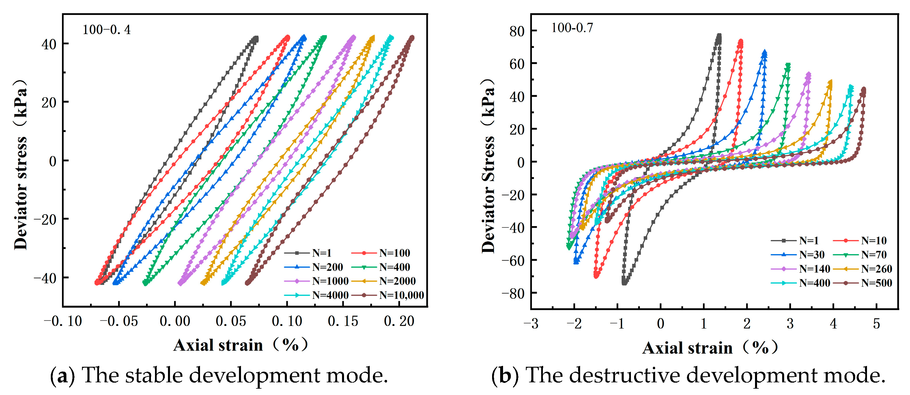
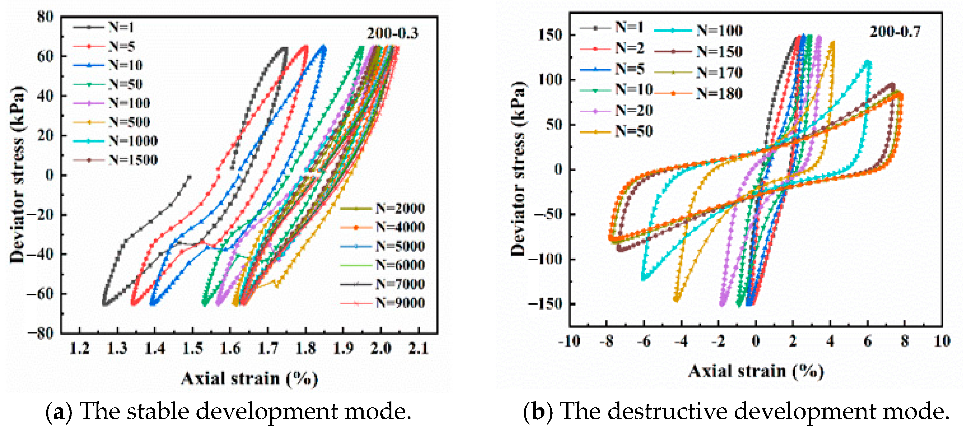
Apart from the cyclic stress path, the hysteresis loop is a crucial parameter for dynamic properties of soil. It plays a vital role in the investigation of accumulated deformation, stiffness degradation, and energy dissipation of submarine soil under cyclic loads. Figure 7 and Figure 8 present the hysteresis curves of marine silt clay and completely weathered granite subjected to varying consolidation pressures and cyclic loads, highlighting two distinct evolutionary patterns.
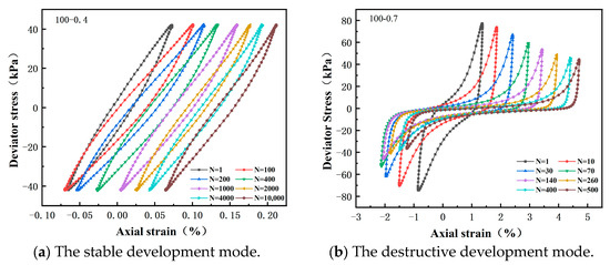
Figure 7.
Hysteresis loop of submarine silt clay with different development modes.
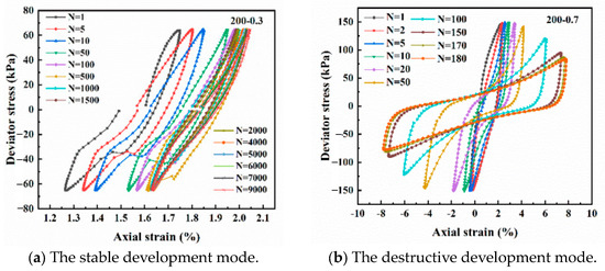
Figure 8.
Hysteresis loop of completely weathered granite with different development modes.
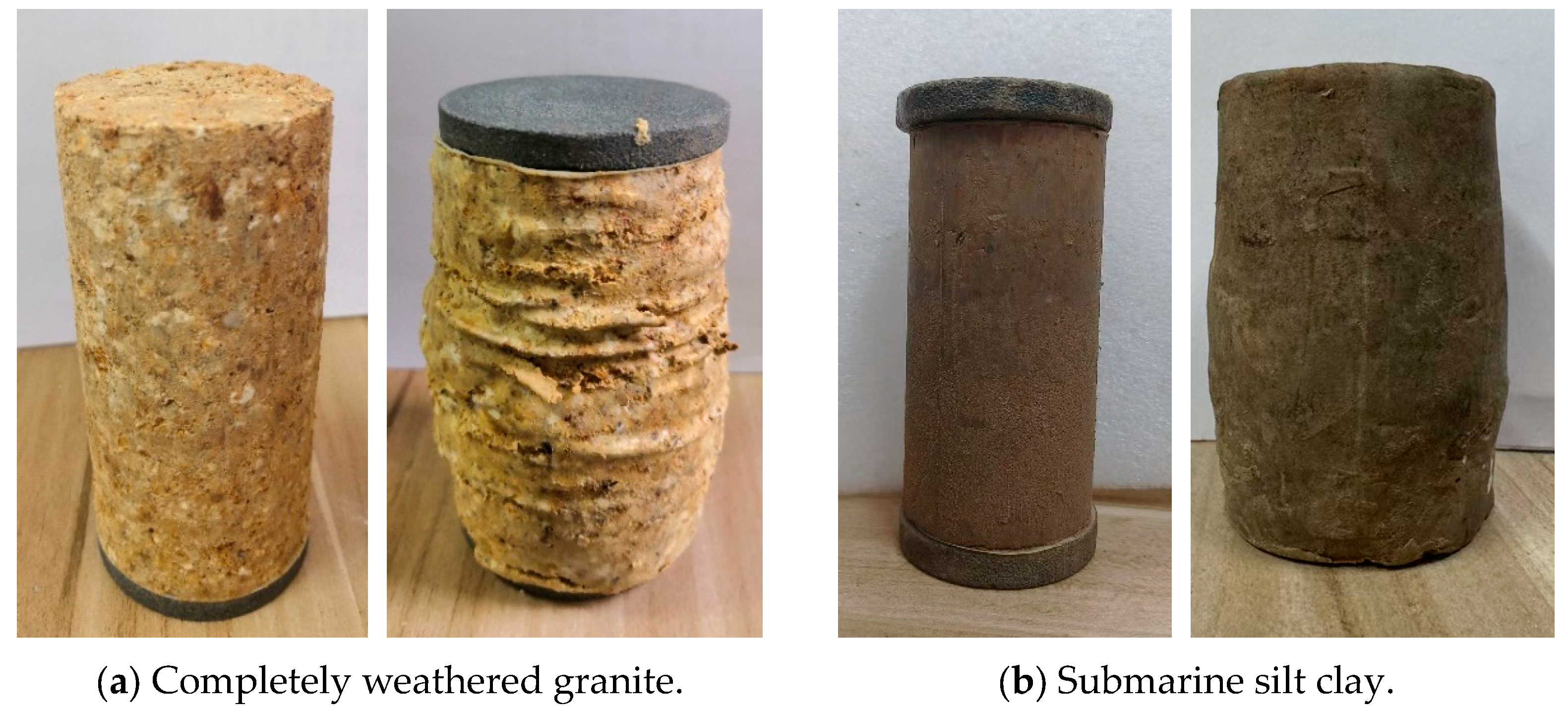
Under conditions of low cyclic stress ratio (CSR), submarine soils are characterized by the stable development mode, as shown in subgraph (a) of Figure 7 and Figure 8. Under continuous low-intensity cyclic loads, the accumulated strain gradually increases, resulting in a parallel rightward shift in the hysteresis loop. However, the overall shape of the hysteresis loop typically remains “spindle-shaped”, and the deviatoric stress can attain the predetermined values. The external dynamic loads caused significant shifts in the hysteresis curve to the right in the early stages of dynamic triaxial tests; however, since the magnitude of the applied external cyclic loads are relatively small, the internal structures of soil samples rapidly return to the balanced state without failure. Consequently, as the cycle number gradually increases, the strain no longer exhibits significant increase, resulting in the hysteresis curves essentially overlapping in the later stages of the tests. During the parallel rightward movement of the hysteresis curves, both the area and slope remained relatively consistent, indicating that the damping and stiffness do not change significantly. Furthermore, the external shapes of the soil samples after the test maintain the standard cylindrical form, as observed before the test (Figure 9).
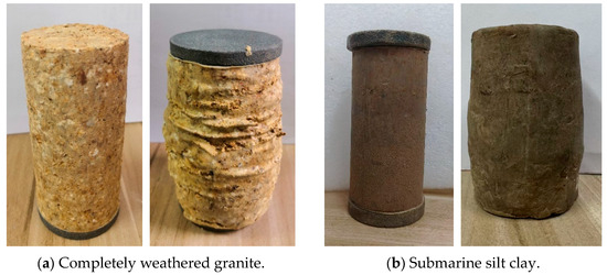
Figure 9.
External shape of submarine testing soil samples after tests.
With the increase in CSR, the development mode of submarine soil hysteresis curves transitions from the stable mode to the destructive mode. The large external cyclic loads significantly accelerate the axial strain, leading to the accumulated strain reaching higher levels after fewer cycles. With the increases in cycle number, the testing soil approaches a critical state, leading to the potential destruction of soil internal structures. The hysteresis loop no longer shifts parallel to the right, and the backbone curve of the hysteresis loop gradually tilts and rotates clockwise around the coordinate origin, resulting in a progressive decrease in stiffness, as shown in subgraph (b) of Figure 7 and Figure 8. In contrast to the stable development mode, the hysteresis curve transitions from the initial spindle shape to the anti-S shape. The overall width and area of the hysteresis curves gradually increase, indicating that the energy consumption is huge, and the soil is seriously damaged. The soil has been seriously deformed in appearance after tests, and the soil interior structure cannot bear the external loads, as illustrated in Figure 9.
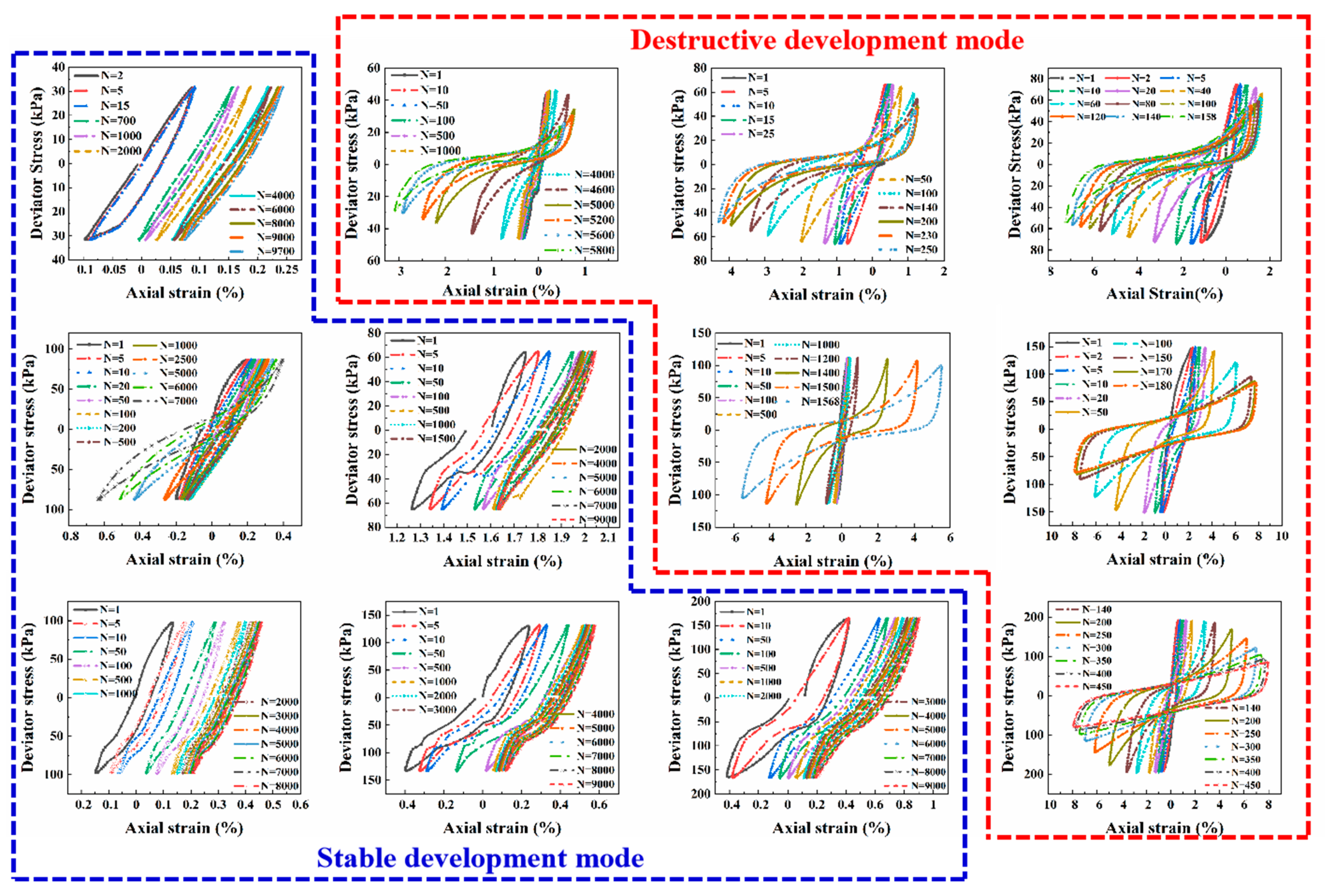
According to the partition method of the development mode, the cyclic behaviors of submarine soils from offshore wind farms can be accurately divided into a destructive and stable mode. For example, the completely weathered granite under the following testing conditions belongs to the stable development mode, i.e., 100 kPa-CSR0.3, 200 kPa-CSR0.3, 200 kPa-CSR0.4, 300 kPa-CSR0.3, 300 kPa-CSR0.4, and 300 kPa-CSR0.5. On the contrary, the following is for the destructive development mode: 100 kPa-CSR0.4, 100 kPa-CSR0.5, 100 kPa-CSR0.6, 100 kPa-CSR0.7, 200 kPa-CSR0.5, 200 kPa-CSR0.6, 200 kPa-CSR0.7, 300 kPa-CSR0.6, and 200 kPa-CSR0.7, as shown in Figure 10.
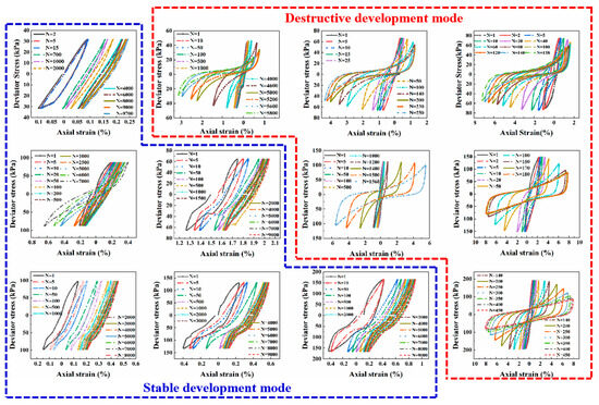
Figure 10.
Cyclic development mode partition of completely weathered graine.
The stable and destructive development modes are clearly distinct, and there is a CSR threshold that can lead to soil failure. The dynamic stress intensity required for soil to reach the critical state of failure under cyclic loading is defined as the critical cyclic stress ratio (CSR). The stress ratio serves as a key demarcation between soil sample failure and is widely utilized as a criterion in engineering design, and the critical CSRs of five types of submarine soil from offshore wind farms under different confining pressures are illustrated in Table 3.
Table 3.
Critical CSRs of submarine soils from offshore wind farms.
4. Methodology
4.1. Random Forest
Random forest (RF) is an integrated learning algorithm for solving classification and regression problems, and an integrated learning model that uses multiple decision trees to train and predict samples as basic classifiers [30]. In a decision tree, a decision is made at each node, and a split is performed iteratively until the node reaches a state of purity, meaning that it contains only samples of a single class. Like other data-driven methodologies, this approach necessitates the use of training data to construct the model. Each tree in the random forest (RF) algorithm is built using a bagging technique known as bootstrapping, which involves sampling the training data with replacement to create multiple subsets for training individual trees. Due to its straightforward architecture and superior performance compared to many other machine learning techniques, random forest has been extensively applied across various domains.
4.2. Gradient Boosting Decision Tree
Gradient boosting decision tree (GBDT), also named Multiple Additive Regression Tree (MART), is an iterative decision tree algorithm which consists of multiple decision trees [31]. The algorithm optimizes the function in the function space according to the continuous optimization gradient of the parameters in the parameter space. The main method is to create CART trees by introducing negative loss function gradients into the current model, in order to reduce the gap between the model and the actual labeling. The basic logic is based on residual learning, reducing the residuals with the help of iteration, forming a regression decision tree by optimizing the direction of the gradient, and finally accumulating the results of all the regression trees obtained to achieve the final model. Through continuous iteration, accurate results are obtained, and at the same time, in each iteration, with the help of the gradient descent method, the prediction weights of the error samples are assigned, so that each round of iteration error is smaller than that of the previous round.
4.3. Modeling Development
Based on the testing results of dynamic triaxial tests of five type marine soils, 78 hysteresis curve shape data were obtained. In the machine learning-based prediction model, the soil physical property parameters (liquid limit, plastic limit, and water content) and the testing conduction parameters (circumferential pressure, CSR) are set as the model inputs, and the shape of the hysteresis curves (stable mode and destructive mode) is reviewed as the outputs. Therefore, the rapid identification method for the hysteresis curve of marine soil is established. In training the RF and GBDT models, the experimental data are divided into the training set and the test set according to the ratio of 7:3. Then, the test set is used to test the generalization ability of the established model, and the training set data are used to train and optimize the model using a five-fold cross verification method, following the steps given below.
(1) The training set data are randomly divided into 5 subgroups.
(2) Four subgroups are set as the training set, and the remaining one is reviewed as the verification set.
(3) Repeat step (2) 4 times by selecting each subgroup in turn as a validation set.
(4) The mean square error (MSE) was calculated as an index to assess the accuracy of each model with different combinations of hyperparameters.
(5) Finally, the minimum MSE value is determined, and its corresponding hyperparameters constitute the optimal combination.
In order to obtain the more accurate discriminant model for the hysteresis curve, the hyperparameters of the RF and GBDT models are optimized by using the grid search method, and the hyperparameter selection ranges of the RF algorithm and the GBDT algorithm are shown in Table 4.
Table 4.
Selection range of hyperparameter.
4.4. Model Evaluation Indexes
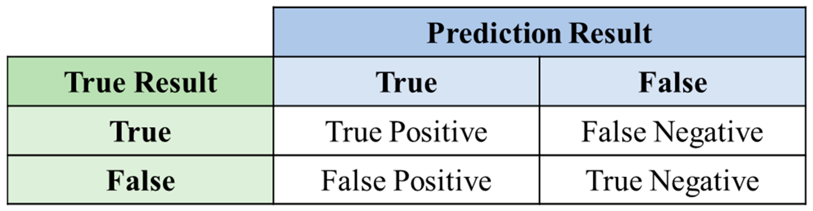
The confusion matrix is an important tool for evaluating the performance of classification models, which clearly presents the classification results of the model in a matrix format, as shown in Figure 11. In the matrix, True Positive (TP) means that the true category of the sample is positive, and the model recognizes it as a positive example. False Negative (FN) means that the true category of the sample is positive, but the model recognizes it as a negative example. False Positive (FP) means that the true category of the sample is negative, but the model recognizes it as a positive example. True Negative (TN) means that the true category of the sample is negative, and the model recognizes it as a negative example.

Figure 11.
Schematic diagram of the classification matrix.
In the study, the accuracy, precision, recall, F1-score, receiver operating characteristic (ROC), and area under the ROC curve (AUC) are selected as the model evaluation indexes to evaluate the classification performance of the established model.
Accuracy is the most common evaluation index for classification models, which is on behalf of the proportion of samples correctly predicted by the model to the total number of samples. Precision refers to the proportion of actual positive cases among all samples predicted as positive by the model. Recall refers to the proportion of samples that are actually positive cases and are correctly predicted as positive by the model. F1-score is the harmonic mean of precision, and recall and is a comprehensive index for evaluating the performance of the classification model.
Receiver operating characteristic curve (ROC) is a curve drawn with the True Positive Rate (TPR) as the vertical coordinate and the False Positive Rate (FPR) as the horizontal coordinate. The closer the ROC curve is to the upper left corner, the better the model performance is, and the larger the corresponding AUC is.
5. Results and Discussion
The fast-discriminating method for the hysteresis curve morphology of submarine soil materials based on machine learning is proposed. In order to optimize the hyperparameters of the machine learning algorithm, the grid search is used as the hyperparameter tuning method, and the results of the hyperparameter optimization of RF and GBDT algorithms are shown in Table 5.
Table 5.
Optimization results for RF model and GBDT model.
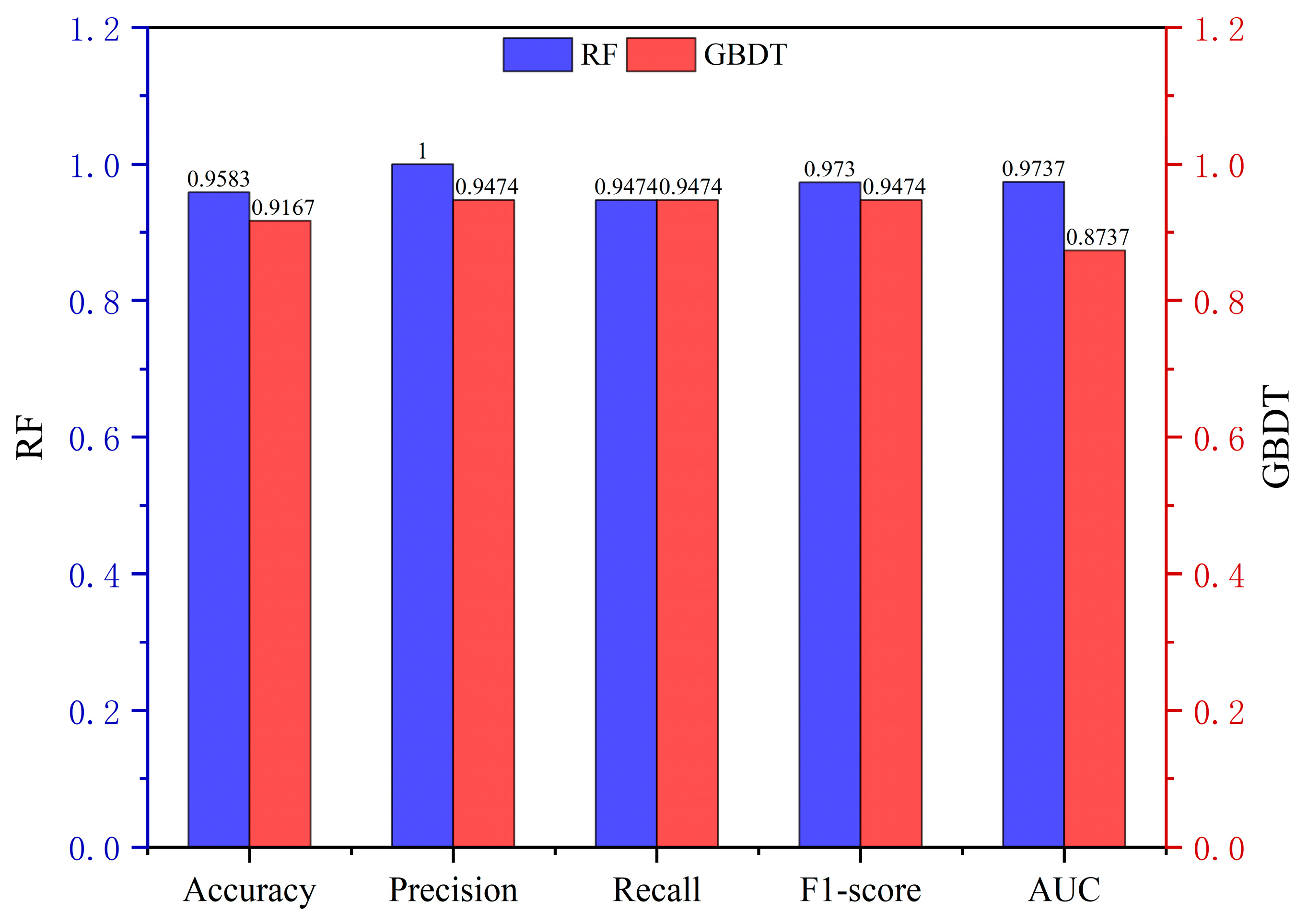
The above optimal parameters are inputted into the RF and GBDT models, and the classification prediction results of the two models on the training and test sets are shown in Table 6 and Figure 12. It can be noted that both the RF model and the GBDT model can achieve completely correct classification results when predicting the training set data. When predicting the test set data, the five evaluation indexes of the RF model are higher than or equal to that of the GBDT model. Compared to the GBDT model, five evaluation indexes of RF model are improved by 4.8%, which indicates that the RF model has a better generalization ability and higher accuracy than the GBDT model in discriminating the hysteresis curve shape.
Table 6.
Discrimination accuracy of hysteresis loop.
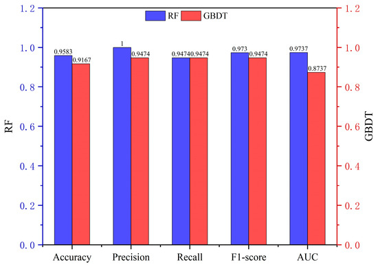
Figure 12.
Discrimination accuracy of RF and GBDT hysteresis curve.
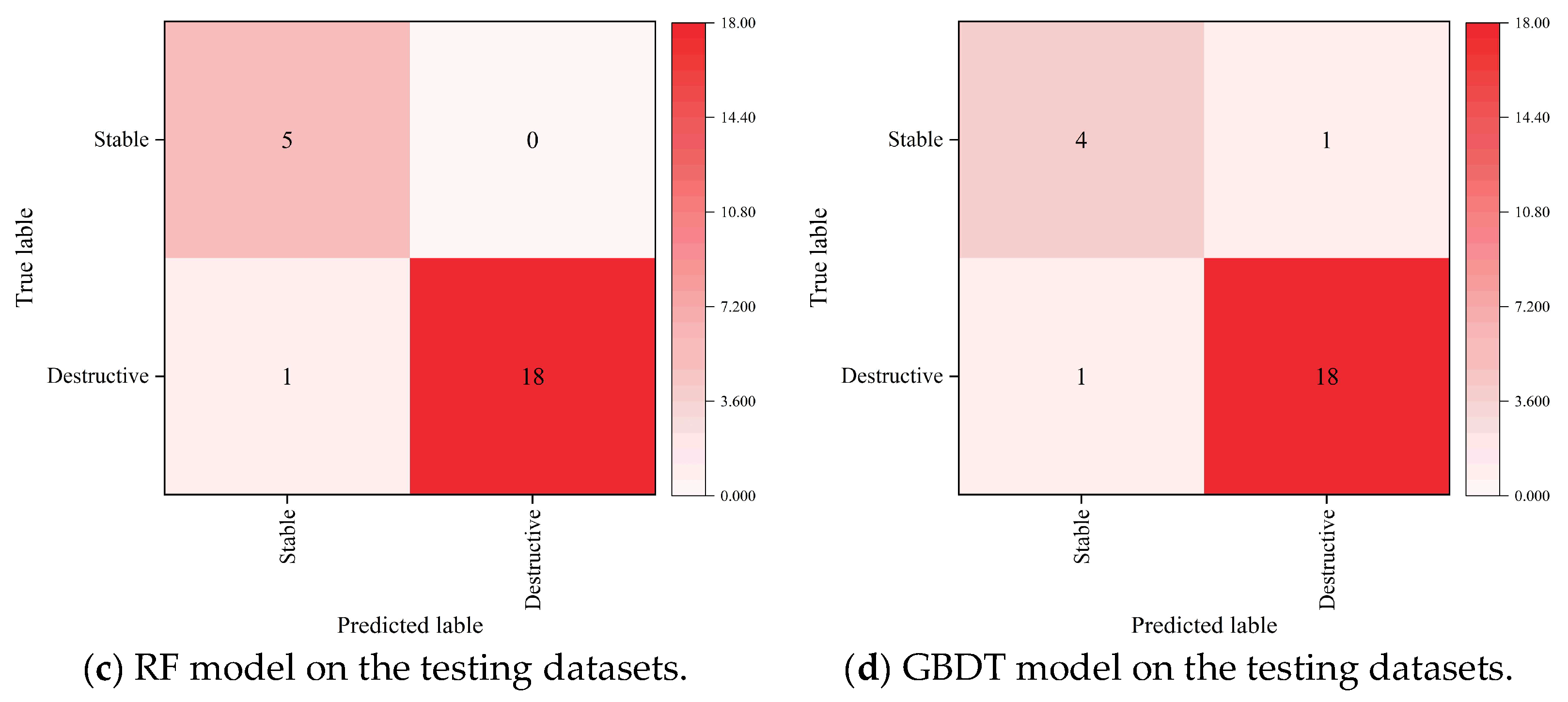
Figure 13 illustrates the confusion matrix of the classification results of the RF model and the GBDT model. Figure 13a,c show the prediction results of the RF model on the training and testing datasets, respectively. Figure 13b,d show the prediction results of the GBDT model on the training and testing datasets, respectively. It can be seen that the predicting accuracy of the RF and GBDT models is 100% when predicting the training set data. When predicting the testing set data, there is one wrong classification in the RF model and two wrong classifications in the GBDT model.
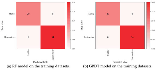
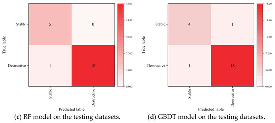
Figure 13.
Confusion matrix of RF model and GBDT model prediction results.
Figure 14 presents the ROC curves of the RF model and the GBDT model prediction results. The ROC curves of the RF and GBDT training set data are exactly the same, whereas the ROC curve of the RF model on the testing set is closer to the upper left than that of the GBDT model. The AUC of the RF model on the test set is 0.9737, and that of the GBDT model is 0.8737. The random forest (RF) model demonstrates superior generalization capabilities compared to the gradient boosting decision tree (GBDT) model, resulting in enhanced predictive accuracy for the RF model. RF is capable of effectively handling the nonlinear relationships in soil hysteresis loop data, and it reduces the risk of overfitting, particularly when the sample size is small or under challenging conditions, thus providing more accurate predictive results.
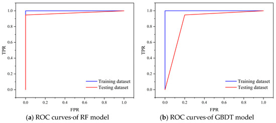
Figure 14.
ROC curves of RF model and GBDT model prediction results.
6. Conclusions
In total, 78 representative submarine soil samples were collected from four offshore wind farms, and cyclic behaviors under different confining pressures and CSR were investigated. Based on the dynamic triaxial test results, the machine learning-based partition models for cyclic development mode were established, and the discrimination accuracy of the hysteresis loop were discussed. The main conclusions obtained in the study are given below.
(1) The cyclic behaviors of submarine soils present two distinctly different development modes under various cyclic loads, i.e., the stable development mode under small cyclic loads, and the destructive development mode under large cyclic loads.
(2) The critical CSRs of completely weathered granite under 100 kPa, 200 kPa, and 300 kPa are 0.35, 0.45, and 0.55, and that of silt clay are 0.65, 0.55, and 0.45.
(3) The RF model has a better generalization ability and higher accuracy than the GBDT model in discriminating the hysteresis loop of submarine soil.
Although this study has achieved some constructive results, there are still many deficiencies. The actual marine environment is complex and changeable, including the combined effects of waves, tides, currents, and other factors. Most of the existing studies focus on the experiments under single factor or simplified conditions, and there is a lack of in-depth research on the coupling effect of multiple factors. The experimental results under laboratory conditions may be different from the actual field conditions. Although a cycle expansion mode division model based on machine learning is established, there is still room for improvement in the refinement and optimization of the model. In order to improve the applicability of the laboratory model in practical engineering, future research can combine the field measured data to verify and correct the laboratory model.
Author Contributions
Conceptualization, B.H. (Ben He) and B.H. (Bo Han); Methodology, M.L. and B.H. (Bo Han); Software, Z.Z.; Formal analysis, M.L., Z.Z. and X.Y.; Writing—original draft, B.H. (Ben He) and M.L.; Writing—review & editing, Z.Z. and X.Y.; Funding acquisition, B.H. (Bo Han). All authors have read and agreed to the published version of the manuscript.
Funding
This research was funded by the China Postdoctoral Science Foundation (2023M742093), Postdoctoral Innovation Project of Shandong Province (SDCX-ZG-202302004), National Natural Science Foundation of China Joint Program (U23A20663), National Natural Science Foundation of China (52409161; 52171266; 52271294), and “Pioneer” and “Leading Goose” R&D Program of Zhejiang (NO. 2024C03031).
Institutional Review Board Statement
Not applicable.
Informed Consent Statement
Not applicable.
Data Availability Statement
Data are contained within the article.
Conflicts of Interest
Author He Ben was employed by the company Power China Huadong Engineering Corporation Limited HDEC. The remaining authors declare that the research was conducted in the absence of any commercial or financial relationships that could be construed as a potential conflict of interest.
References
- Liu, D.; Liu, M.; Xu, X.; Wang, J.; Fan, C.; Li, X.; Han, J. Future prospects research on offshore wind power scale in China based on signal decomposition and extreme learning machine optimized by principal component analysis. Energy Sci. Eng. 2020, 8, 3514–3530. [Google Scholar] [CrossRef]
- Jansen, M.; Staffell, I.; Kitzing, L.; Quoilin, S.; Wiggelinkhuizen, E.; Bulder, B.; Riepin, I.; Müsgens, F. Offshore wind competitiveness in mature markets without subsidy. Nat. Energy 2020, 5, 614–622. [Google Scholar] [CrossRef]
- GWEC.NET. Associate Sponsors Podcast Sponsor Leading Sponsor Supporting Sponsor Co-Leading Sponsor (n.d.). Available online: www.gwec.net (accessed on 1 January 2025).
- Wang, Y.; Zhang, S.; Yin, S.; Liu, X.; Zhang, X. Accumulated Plastic Strain Behavior of Granite Residual Soil under Cycle Loading. Int. J. Geomech. 2020, 20, 04020205. [Google Scholar] [CrossRef]
- Yan, X.; Zhang, N.; Ma, K.; Wei, C.; Yang, S.; Pan, B. Overview of Current Situation and Trend of Offshore Wind Power Development in China. Power Gener. Technol. 2024, 45, 1. [Google Scholar] [CrossRef]
- Ma, H.; Deng, Y.; Chang, X. Effect of long-term lateral cyclic loading on the dynamic response and fatigue life of monopile-supported offshore wind turbines. Mar. Struct. 2024, 93, 103521. [Google Scholar] [CrossRef]
- Zhang, X.; Zhou, R.; Han, Y. Study on p-y curve of large diameter pile under long-term cyclic loading. Appl. Ocean Res. 2023, 140, 103736. [Google Scholar] [CrossRef]
- Xiao, W.; Wu, K.; Xu, W.; Liu, Y.; Lu, H.; Chen, R. Experiment and analysis on dynamic characteristics of marine soft clay. Mar. Georesources Geotechnol. 2024, 12, 1549. [Google Scholar] [CrossRef]
- Yang, J.; Cui, Z.D.; Xi, B.; Song, W. Experimental study on cyclic triaxial behaviors of saturated soft soil considering time intermittent and variable confining pressure. Soil Dyn. Earthq. Eng. 2024, 179, 108508. [Google Scholar] [CrossRef]
- Dai, S.; Yu, X.; Han, B.; He, B. Cyclic behavior of seabed building material of offshore wind farm in rock-based sea area: Submarine completely weathered granite. Ocean Eng. 2024, 296, 117024. [Google Scholar] [CrossRef]
- Jiang, L.; Sun, J.; Liu, X. Pore-space microstructure and clay content effect on the elastic properties of sandstones. Pet. Sci. Technol. 2012, 30, 830–840. [Google Scholar] [CrossRef]
- Liu, F.; Cai, Y.; Xu, C.; Wang, J. Research on the attenuation law of dynamic elastic modulus of soft soil under cyclic loading. J. Zhejiang Univ. Eng. Ed. 2008, 9, 1479–1483. [Google Scholar]
- Samir El-Kady, M.; ElMesmary, M.A. Cyclic strengths for high density soils related to pore water pressure. Innov. Infrastruct. Solut. 2018, 3, 46. [Google Scholar] [CrossRef]
- Kim, J.; Yoo, M. Development of Excess Pore Water Pressure in Sand during K0-Controlled Cyclic Loading. KSCE J. Civ. Eng. 2024, 28, 1790–1796. [Google Scholar] [CrossRef]
- Dai, S.; Yu, X.; Han, B.; Zhang, Z.; He, B.; Lin, M. Failure criterion of submarine completely weathered granite under cyclic loads in rock-based sea area. Ocean Eng. 2024, 313, 119422. [Google Scholar] [CrossRef]
- Gao, H.; Sun, J.; Stuedlein, A.W.; Li, S.; Wang, Z.; Liu, L.; Zhang, X. Flowability of Saturated Sands under Cyclic Loading and the Viscous Fluid Flow Failure Criterion for Liquefaction Triggering. J. Geotech. Geoenviron. Eng. 2024, 150, 04023130. [Google Scholar] [CrossRef]
- Jiao, G.; Zhao, S.; Ma, W.; Luo, F.; Kong, X. The evolution law of hysteresis loop of frozen soil under cyclic loading. J. Geotech. Eng. 2013, 7, 1343–1349. [Google Scholar]
- Bocheńska, M.; Srokosz, P.E. Artificial Neural Network-aided Mathematical Model for Predicting Soil Stress-strain Hysteresis Loop Evolution. Civ. Environ. Eng. Rep. 2024, 34, 120–135. [Google Scholar] [CrossRef]
- Dai, S.; Han, B.; Li, N.; Wang, B.; He, B.; Liu, J. Morphologic analysis of hysteretic behavior of China Laizhou Bay submarine mucky clay and its cyclic failure criteria. Bull. Eng. Geol. Environ. 2022, 81, 52. [Google Scholar] [CrossRef]
- Doygun, O.; Brandes, H.G. High strain damping for sands from load-controlled cyclic tests: Correlation between stored strain energy and pore water pressure. Soil Dyn. Earthq. Eng. 2020, 134, 106134. [Google Scholar] [CrossRef]
- Alyami, M.; Onyelowe, K.; AlAteah, A.H.; Alahmari, T.S.; Alsubeai, A.; Ullah, I.; Javed, M.F. Innovative hybrid machine learning models for estimating the compressive strength of copper mine tailings concrete. Case Stud. Constr. Mater. 2024, 21, e03869. [Google Scholar] [CrossRef]
- Inqiad, W.B.; Dumitrascu, E.V.; Dobre, R.A.; Khan, N.M.; Hammood, A.H.; Henedy, S.N.; Khan, R.M.A. Predicting compressive strength of hollow concrete prisms using machine learning techniques and explainable artificial intelligence (XAI). Heliyon 2024, 10, e36841. [Google Scholar] [CrossRef] [PubMed]
- Ozkaynak, M.I.; Yilmaz, Y. Prediction of resilient modulus with pre-post experimental data of undisturbed subgrade soils using machine learning algorithms. Transp. Geotech. 2024, 49, 101396. [Google Scholar] [CrossRef]
- Wang, X.; Dong, X.; Zhang, Z.; Zhang, J.; Ma, G.; Yang, X. Compaction quality evaluation of subgrade based on soil characteristics assessment using machine learning. Transp. Geotech. 2022, 32, 100703. [Google Scholar] [CrossRef]
- Sun, J.; Zhang, R.; Zhang, A.; Wang, X.; Wang, J.; Ren, L.; Zhang, Z.; Zhang, Z. Rock strength prediction based on machine learning: A study from prediction model to mechanism explanation. Measurement 2024, 238, 115373. [Google Scholar] [CrossRef]
- Hansen, T.F.; Erharter, G.H.; Liu, Z.; Torresen, J. A comparative study on machine learning approaches for rock mass classification using drilling data. Appl. Comput. Geosci. 2024, 24, 100199. [Google Scholar] [CrossRef]
- Arif, M.; Jan, F.; Rezzoug, A.; Afridi, M.A.; Luqman, M.; Khan, W.A.; Kujawa, M.; Alabduljabbar, H.; Khan, M. Data-driven models for predicting compressive strength of 3D-printed fiber-reinforced concrete using interpretable machine learning algorithms. Case Stud. Constr. Mater. 2024, 21, e03935. [Google Scholar] [CrossRef]
- Zhang, Z.; Yu, X.; Han, B.; Dai, S. Cumulative strain intelligent evaluation of marine soil from offshore wind farms based on enhanced machine learning. Appl. Ocean Res. 2024, 153, 104265. [Google Scholar] [CrossRef]
- Wang, X.; Zhang, Z.; Song, Z.; Li, J. Engineering properties of marine soft clay stabilized by alkali residue and steel slag: An experimental study and ANN model. Acta Geotech. 2022, 17, 5089–5112. [Google Scholar] [CrossRef]
- Zhao, Y.; Teng, C. Classification of soil layers in Deep Cement Mixing using optimized random forest integrated with AB-SMOTE for imbalance data. Comput. Geotech. 2025, 179, 106976. [Google Scholar] [CrossRef]
- Huang, C.; Du, H.; Li, L.; Ni, J.; Sun, Y. Application of tree-based methods in predicting the surface settlement arising from the tunnel excavation with large mix-shield. Soils Found. 2023, 63, 101379. [Google Scholar] [CrossRef]


Disclaimer/Publisher’s Note: The statements, opinions and data contained in all publications are solely those of the individual author(s) and contributor(s) and not of MDPI and/or the editor(s). MDPI and/or the editor(s) disclaim responsibility for any injury to people or property resulting from any ideas, methods, instructions or products referred to in the content. |
© 2025 by the authors. Licensee MDPI, Basel, Switzerland. This article is an open access article distributed under the terms and conditions of the Creative Commons Attribution (CC BY) license (https://creativecommons.org/licenses/by/4.0/).