Abstract
As the demand for high-precision measurements of refractive index variations in marine environments increases, eliminating potential sources of measurement errors has become an urgent issue. One of these error sources is the impact of optical path length perturbations. This study investigates the effect of optical path perturbations on the accuracy of the measurements using the interference method. By establishing an error analysis model, this study analyzes the systematic errors induced by optical path perturbations and verifies the error patterns under different refractive index variations through simulations and experiments. The results show that the errors introduced by optical path perturbations are linearly related to the magnitude of the perturbations, and the error increases as the magnitude of the perturbation grows. The error becomes negligible when the magnitude of the optical path perturbations relative to the measurement zone length is one order of magnitude smaller than the refractive index measurement accuracy. The experimental and simulation results are consistent, validating the accuracy of the model. This indicates that in high-precision seawater refractive index measurements using the interference method, perturbations in the measurement region cannot be ignored, and it is difficult to achieve higher measurement precision through physical vibration isolation alone, highlighting the urgent need for new solutions.
1. Introduction
Seawater salinity serves as a fundamental physical parameter essential for characterizing oceanographic properties. Long-term monitoring of seawater salinity is crucial for assessing the health of marine ecosystems, advancing global climate change research, and exploring the dynamic behavior of oceanic systems [1,2,3]. Given the fundamental role of salinity in the characterization of seawater, it is imperative to ensure the precise measurement of this parameter [4,5]. Research has demonstrated that the latitudinal gradient of salinity in the deep sea along 149° E in the western North Pacific Ocean is approximately 0.0002 g/kg [6]. This finding indicates that the salinity variations in the deep sea are exceedingly slight, thereby underscoring the necessity for methodologies that enable the realization of high-precision seawater salinity measurements. Existing seawater salinity measurements, including the traditional conductivity method with a measurement resolution of 0.004 g/kg [7], acoustic-based salinity sensors with an uncertainty of 0.012 g/kg [8], and optical-based double-V refractometers with a salinity resolution of 0.001 g/kg [9], have not yet succeeded in surpassing the aforementioned measurement indices. However, the results suggest that a measurement method based on optical means holds considerable promise in surpassing the current measurement indices of seawater salinity. As demonstrated by the empirical equation between the optical refractive index and salinity proposed by Millard and Seaver (1990) [10], optical means have become an effective method of measuring seawater salinity. Presently, interferometry is a promising technique for measuring the refractive index of seawater. It has the potential to achieve a salinity resolution of 0.0002 g/kg, which corresponds to a refractive index resolution of approximately RIU [11]. In a laboratory setting, Mahrt and Kroebel (1984) [12] employed Michelson interferometric structures to obtain refractive index measurements of liquids at varying salinities, achieving a refractive index resolution of RIU through the streak counting method. Building upon this work, Hiroshi Uchida (2019) [13] and colleagues further refined the Michelson interferometric structure, integrating a spectral analyzer to attain a refractive index measurement accuracy of RIU. In our previous research, we designed a seawater refractive index sensor based on the principle of optical heterodyne interference [14]. The experimental findings demonstrated that the sensor exhibited a measurement accuracy of RIU under laboratory conditions, thereby substantiating its capacity to meet the measurement requirements for seawater salinity under laboratory conditions. However, the environment encountered during in situ oceanic measurements differs from that of laboratory conditions. In the ocean environment, factors such as waves, ocean circulation, complex climate change, ocean pressure, and marine life contribute to an unstable measurement environment, thereby causing the interference structure to become unstable. The geometric length of the light passing through the measurement area of the seawater is significantly disturbed, leading to a reduction in the accuracy of the seawater refractive index measured by the interferometer. Achieving a measurement accuracy of RIU is a formidable challenge. Consequently, within the marine environment, the implementation of optical interferometry necessitates the minimization of perturbations to the geometric length of the optical path within the measurement area, thereby enhancing the precision of measurements of the refractive index of seawater. In previous studies, Seaver and Vlasov (1997) [15] designed and manufactured Lamina-2 based on the Mach–Zehnder interferometer structure. The resultant measurement of the seawater refractive index, obtained in situ at a depth of 400 m, yielded an accuracy of approximately RIU. In a subsequent study, Hiroshi Uchida et al. (2019) [13] predicted and estimated the results obtained by the spectrometer, and the accuracy can reach a RIU in situ measurement in the deep sea of the North Pacific (up to 40 MPa). In a related study, Yang and Xu (2024) [16] employed a sapphire window structure based on the Michelson interferometer structure to offset the change in the optical path length in the deep sea. In situ measurements at a depth of 4000 m for a period of three months revealed an error of approximately RIU in the measurement of the seawater refractive index. While the aforementioned teams have obtained favorable outcomes in marine environment tests, a discrepancy persists with the anticipated value of RIU.
In order to explore the influence of the marine environment on the geometric length of light passing through the seawater measurement area and further improve the measurement accuracy of the optical interferometry method in the measurement of the seawater refractive index, this paper, based on the previously completed seawater refractive index sensor, carried out a study on the influence of optical path geometric length perturbation on the seawater refractive index measurement error. This study established a model to analyze the error in measuring the refractive index of seawater. It also conducted specific simulations and experiments to analyze the systematic error introduced by geometric length perturbations in the optical path. This study provides a theoretical and empirical foundation for the design of a high-precision in situ measurement system for the refractive index of seawater in complex marine environments.
2. Mathematical Model and Simulation
2.1. Principle of Interferometry to Measure the Refractive Index of Seawater
In our previous research, we designed a seawater refractive index sensor based on the principle of heterodyne interference and demonstrated the effectiveness of this approach through experiments [14]. The measurement structure and schematic diagram of the sensor are shown in Figure 1.
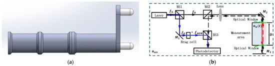
Figure 1.
Seawater refractive index sensor based on the interferometry measurement principle. (a) (b) Schematic diagram of the principle of measuring the refractive index of seawater based on interferometry.
The principle is shown in Figure 1b. The frequency of the laser emitted from the laser source is . The laser beam is split into two beams, the transmitted and reflected beams, by the beam splitter BS1. The reflected beam, serving as the reference beam, is reflected by mirror M1 and then passes through the Bragg cell, generating a frequency shift of . The beam is then reflected by the beam splitter BS3 onto the surface of the photodetector. The transmitted beam acts as the measurement beam, passing through the beam splitter BS2, being collimated by a lens system, and directed by mirror M2 so that it vertically enters the measurement area. After passing through the optical windows in front and behind the measurement area, the beam reaches the bottom reflective surface M3. Then, the beam is reflected by M3, and the reflected beam travels back through the measurement area, mirror M2, beam splitter BS2, and beam splitter BS3 to reach the photodetector, where it interferes with the reference beam. As shown in the diagram, the blue path represents the path of the reference light traveling through air, with a length of , the black path represents the path of the measurement light traveling through air, with a length of , and the red path represents the path of the measurement light traveling through the measurement area. D is the constant length of the measurement area. is the refractive index of air, and is the refractive index of the seawater to be measured in the measurement area. The intermediate frequency signal obtained by the detector is as follows:
Here, and are the electric field intensities of the reference beam and the measurement beam, respectively, while and are the initial phase values of the reference beam and the measurement beam, respectively. The phase shift is obtained by phase demodulation of the intermediate frequency signal using the arctangent method as follows:
Due to the presence of and , is an unknown quantity. The direct extraction of the refractive index information from Equation (2) is, therefore, infeasible without eliminating . To address this, we differentiate Equation (2) to remove the term, and the rate of change of the refractive index with respect to time is obtained.
In Equation (3), the rate of change of the refractive index with respect to time is positively correlated with the rate of change of the phase with respect to time.
2.2. Error Model of Seawater Refractive Index Measurement Due to Perturbation of the Optical Path Geometric Length
In practical measurements, the interferometer is continuously exposed to the marine environment, where it is influenced by unstable measurement conditions, leading to minute variations in the position of the optical windows in the measurement area. When the position of the optical window in the measurement area shifts slightly in a particular direction, the optical path length in the air experiences an inverse change. As a result, the different small positional variations of the optical windows on both sides of the measurement area can be collectively regarded as a perturbation (t) within the measurement area, which simultaneously induces a reverse perturbation in the air.
Assume that the path length traveled by the beam through the measurement area consists of a constant quantity and the optical path geometric length perturbation (t). The perturbation is considered positive when the direction of the perturbation aligns with the direction of the beam propagation. can be expressed as follows:
When a small change in the position of the optical window in the measurement area causes a perturbation (t) in the measurement area, a corresponding reverse perturbation is generated in the air. Therefore, the phase information obtained through arctangent demodulation becomes the following:
By differentiating , we obtain the following:
Due to the presence of the unknown quantity (t), Equation (3) is updated as follows:
If the perturbation (t) is not considered during the demodulation process, systematic errors will be introduced. Based on Equations (3) and (7), the difference between the demodulation results with and without considering the perturbation (t) can be calculated as follows:
Substituting Equation (6) into Equation (8) and simplifying yields as follows:
Integrating Equation (9) yields the systematic error in introduced by the optical path geometric length perturbation (hereinafter referred to as systematic error):
An analysis of Equation (10) reveals that since the fixed length of the measurement region serves as a constant, the influence of the geometric length perturbation of the optical path on the systematic error must be quantified relative to the fixed length of the measurement region. Therefore, by defining the variation in the geometric length perturbation of the optical path relative to the fixed length of the measurement region as the relative perturbation and assuming that the refractive index of seawater under test is composed of its initial measured value and a time-dependent variation during the measurement process, the following is obtained:
Then the systematic error of can be expressed as follows:
The analysis shows that the systematic error introduced by the relative perturbation consists of two components. The latter has a small effect on the measurement of the refractive index variation (for example, when the magnitude of is RIU and the magnitude of is , the error introduced by the latter is on the order of RIU, which is much smaller than the expected measurement accuracy of the seawater refractive index of RIU). The component that has a larger impact on the refractive index variation measurement is the former, and this error contribution comes not only from the relative perturbation but also from the initial difference between the air refractive index and the seawater refractive index, . During the measurement process, is a large quantity compared to . In other words, due to the presence of , the effect of the perturbation on the refractive index measurement cannot be easily ignored.
2.3. Simulation Analysis
According to Equation (12), during the simulation, the initial value of the air refractive index is set to 1.000293, the refractive index is set to 1.333, and the refractive index variation changes in magnitude from RIU to RIU in steps. The optical path geometric length perturbation is simulated as harmonic oscillation as follows:
Here, is the perturbation frequency, and is the perturbation amplitude. Then, the relative perturbation is , the ratio is denoted as the amplitude of the relative perturbation amplitude . Based on the above parameter settings, the systematic error under different magnitudes of the refractive index variation is obtained. Substituting Equation (13) into Equation (12) yields the following:
From the equations, it can be analyzed that the systematic error increases linearly with and decreases linearly with the magnitude of . According to the criterion, the systematic error is considered eliminated [17] (pp. 18–19) when the systematic error in the refractive index measurement satisfies the following equation:
It can be concluded that the impact of the optical path geometric length perturbation on the refractive index measurement can be neglected. Here, is the measurement accuracy of the interferometric system. Equation (15) indicates that when this condition is met, it can be concluded that the systematic error will not affect the measurement accuracy of the interferometric system. Based on Equation (15), Table 1 presents the maximum allowable relative perturbation magnitude for each refractive index measurement accuracy under the simulation conditions.

Table 1.
Maximum allowable perturbation magnitude corresponding to the relative perturbation based on the different measurement accuracy of the refractive index.
From Table 1, it can be seen that to achieve a certain measurement accuracy without being affected by the perturbation , the relative perturbation amplitude should be smaller than the refractive index measurement accuracy. This implies that a smaller necessitates a proportionally narrower permissible range of to ensure that systematic errors induced by the geometric path length perturbations remain negligible in the interferometric system. For varying magnitudes of , the permissible amplitude ranges of geometric path length perturbations corresponding to different refractive index measurement accuracies are summarized in Table 2.
Table 2.
Permissible geometric path length perturbation amplitudes as functions of and the refractive index measurement accuracy .
To investigate the specific impact of different relative perturbation amplitudes on the measurement of the refractive index variation, different magnitudes of the refractive index changes were set, and the maximum systematic error was calculated. The range of relative perturbation amplitudes was selected based on Table 1, with magnitudes varying from to in the successive steps. During the simulation, the deviation of the refractive index variation measurement from the true value under the influence of different systematic errors was evaluated. The RMSE (Root Mean Square Error) was used as the evaluation criterion, and its expression is as follows:
where represents the number of measurements, represents the estimated value, and represents the true value. The RMSE values based on different magnitudes of the refractive index variation affected by different relative perturbation amplitudes are calculated using Equation (16), as shown in Table 3.
Table 3.
Maximum systematic error values and RMSE introduced by different perturbation magnitudes under various refractive index variation magnitudes.
Based on the analysis in Table 3, the plot in Figure 2 is generated. Figure 2 illustrates the variation in systematic errors with a relative perturbation amplitude magnitude () under different refractive index variation magnitudes. The different symbols represent different refractive index variation magnitudes. From Figure 2, it can be seen that for the same refractive index variation magnitude, the larger the relative perturbation amplitude, the greater the systematic error in the refractive index variation measurement, and this error exhibits a linear increase on a logarithmic scale.
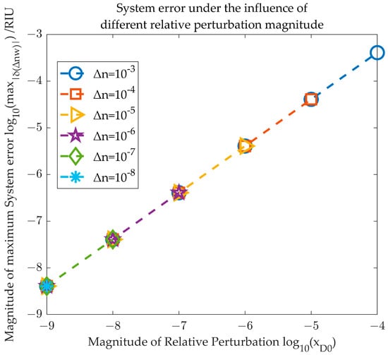
Figure 2.
Changes in systematic errors under different magnitudes of perturbation amplitudes.
3. Experiment
Experimental Design
To validate the correctness of the above conclusions, an experiment was designed to measure the variation in the refractive index of deionized water with temperature within the temperature range of 33 °C to 36 °C using the interferometric method. Tilton et al. (1938) [18] provided an empirical formula.
The refractive index of deionized water is shown as a function of temperature and wavelength, with the laser wavelength set to 632.8 nm.
Using Equation (17), a refractive index measurement precision of RIU can be achieved. Based on this equation, the refractive index variation over time was achieved by heating deionized water using a heating stage. A vibration source (piezoelectric ceramics) was placed on the reflective surface in the measurement area to induce harmonic oscillations of the measurement area’s geometric length, simulating the introduction of optical path length perturbations, and is set to 0.16 m. The experimental setup is shown in Figure 3.
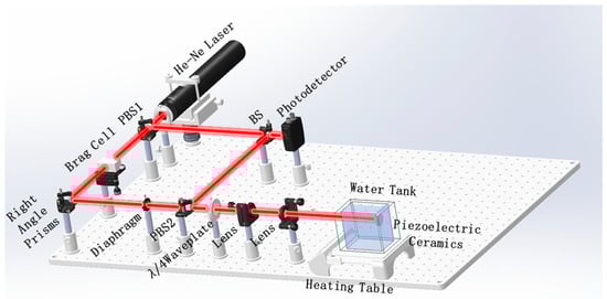
Figure 3.
Experimental scene diagram.
In the experiment, a 632.8 nm wavelength He-Ne laser was used. The beam passed through a polarization beam splitter (PBS1) and was divided into P-polarized and S-polarized light. The P-polarized light was used as the measurement beam, passing through a Bragg cell and a reflection prism before passing through another polarization beam splitter (PBS2). The light is converged by the lens assembly after passing through the quarter-wave plate (QWP), and then the beam passed through a water tank and hit the piezoelectric ceramic (a mirror was attached to the surface of the piezoelectric ceramic), where it was reflected. The reflective surface was aligned to the focal plane of the lens assembly, thereby ensuring that the retroreflected beam could re-enter the exit pupil of the optical system. The reflected beam is collimated into a parallel beam after passing through the lens assembly. Then, the reflected beam passed through a waveplate again, which altered its polarization state, converting it to S-polarized light. The S-polarized light was then reflected by PBS2, reaching a beam splitter (BS), which directed it to the surface of the photodetector. The reference light, reflected by PBS1, then passes through the BS and interferes with the measurement light on the photodetector surface. In this experiment, perturbations were introduced via the piezoelectric ceramic, and the deionized water in the tank was heated using a thermal stage to induce time-dependent variations in the refractive index. These variations exhibited a linear relationship within the temperature range of 33 °C to 36 °C.
In the experiment, a temperature sensor (Mobo Robotics, mSTS-P, with a measurement precision of 0.001 °C) was used for real-time temperature monitoring. Before the experiment, the temperature was used to calibrate the precision of the refractive index measurement by the interferometric method through fitting. As shown in Figure 4, the blue curve represents the temperature variation measured by the temperature sensor, the red curve represents the refractive index variation in deionized water obtained through fitting using Equation (17), and the black curve represents the refractive index variation measured by the interferometric system.
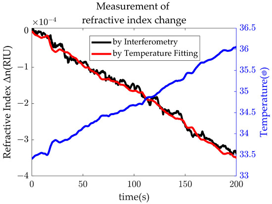
Figure 4.
Temperature Calibrated Refractive Index Measurement Results.
From Figure 5, it can be observed that the larger the relative perturbation amplitude, the greater the introduced systematic error, and the greater the impact on the refractive index variation measurement. According to Equation (15), the systematic errors introduced by relative different perturbation amplitudes under experimental conditions were calculated, and the RMSE of the offset between the refractive index variation measurement results and the temperature-fitted curve was determined for each relative perturbation amplitude. It was found that when the relative perturbation amplitude is on the order of , the refractive index variation measurement precision of RIU can be achieved; when the relative perturbation amplitude is on the order of , the refractive index variation measurement precision of RIU can be achieved. When the relative perturbation amplitude is on the order of , the refractive index variation measurement precision of RIU can be achieved. In other words, under experimental conditions, to achieve a certain order of magnitude in refractive index variation measurement precision, the relative perturbation amplitude should not exceed one order of magnitude greater than the refractive index variation measurement precision, which is consistent with the simulation results.
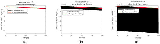
Figure 5.
Effect of relative perturbation on the measurement of refractive index variation. (a) Relative perturbation amplitude under . (b) Relative perturbation amplitude under . (c) Relative perturbation amplitude under .
Simulation parameters were input based on the specific conditions of the experiment, and the simulation results are shown in Table 4.
Table 4.
Comparison results of RMSE under simulation conditions and experimental conditions.
From Table 4, it can be seen that the experimental and simulation results exhibit the same trend, with the measurement precision of the refractive index variation decreasing linearly as the relative perturbation amplitude increases. Furthermore, based on Equation (15), it is found that under laboratory conditions, for refractive index variation at the order of magnitude, relative perturbation amplitudes on the order of can be ignored, which is consistent with the conclusion from the simulation, thus validating the accuracy of the simulation results. A comparison of the systematic errors introduced by relative perturbation amplitudes in both the simulation and experiment is shown in Figure 6.
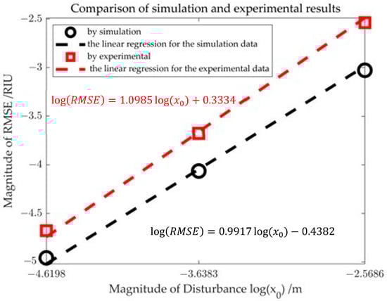
Figure 6.
Comparison chart of simulation results and experimental results.
From Figure 6, it can be seen that the data under experimental conditions show a roughly linear relationship with the simulation data on a logarithmic scale with a similar trend. Both exhibit an increase in RMSE as the relative perturbation amplitude increases. Additionally, fitting the scatter plot, the slope indicates that the two sets of data have a similar linear relationship. However, the slope of the experimental data (1.0985) is slightly greater than that of the simulation data (0.9917), suggesting that the error growth in the experiment is slightly faster than in the simulation setup. The intercept of the data fitting under experimental conditions is 3334, while the intercept under simulation conditions is −0.4382. The difference in intercepts indicates that, in the absence of relative perturbations, the error baseline in the experimental data is higher, which suggests that the experimental process may be affected by environmental noise and other factors.
4. Results and Discussion
According to the theoretical analysis, the systematic error introduced by the geometrical length perturbation in the measurement path when measuring the refractive index variation is related to three factors: the fixed length of the measurement area, the geometrical length perturbation in the measurement path, and the difference between the initial refractive index of the measurement area and the refractive index of air. The fixed length of the measurement zone and the geometric path length perturbation within it combine to form the dimensionless relative perturbation amplitude .
According to the simulation analysis, when assuming the relative perturbation is harmonic vibration, Equation (15) can be used to determine whether the systematic error can be ignored. The calculation shows that to achieve a certain measurement precision without being affected by the perturbation, the relative perturbation amplitude must be smaller than the refractive index measurement precision. Different -values represent different interferometry systems. It has been observed that under a given measurement accuracy of the refractive index, different values lead to varying levels of system tolerance towards geometric length disturbances in the optical path. Specifically, smaller values result in poorer tolerance of the measurement system to geometric length disturbances in the optical path. For different magnitudes of refractive index variations, the maximum systematic error introduced by the relative perturbation was calculated, and it was found that the systematic error increases linearly with the relative perturbation amplitude. Moreover, the same trend is observed for refractive index variations at different magnitudes. An experiment was set up to validate the simulation results. A calibration experiment based on the temperature fitting formula was first conducted. The calibration results showed that the refractive index variation measured by the interferometric method did not deviate from the temperature-fitting results at the magnitude. Further experiments based on the calibration results also showed that, to achieve a certain refractive index variation measurement precision, the relative perturbation amplitude must be at least one order of magnitude smaller than the refractive index measurement precision. If the relative perturbation amplitude exceeds one order of magnitude, the measurement precision at that magnitude cannot be guaranteed. In experiments exploring the impact of different relative perturbation levels on the refractive index variation measurement, it was observed that as the relative perturbation amplitude increases, the systematic error increases, and the impact on the refractive index variation measurement precision also increases. This trend aligns with the simulation results, where both exhibit a similar linear relationship on a logarithmic scale.
5. Conclusions
This paper establishes a theoretical analysis model for the impact of geometrical path length perturbations on refractive index measurements based on the principle of interferometric measurements. Using this theoretical model, a simulation analysis was conducted to evaluate the measurement errors introduced by geometrical path length perturbations. The correctness of the model was verified through experiments, providing potential references for further improving the measurement accuracy of the seawater refractive index. Based on the theoretical analysis, simulation results, and experimental findings, the following conclusions can be drawn:
- (1)
- Due to the presence of , the systematic error introduced by the geometrical path length perturbation in the measurement area cannot be easily ignored.
- (2)
- To achieve an accurate measurement of a certain refractive index change magnitude, the allowable relative perturbation magnitude is always one order of magnitude smaller than the refractive index change magnitude.
- (3)
- The choice of the parameter critically governs the interferometric system’s susceptibility to geometric path length disturbances and must, therefore, be carefully optimized through a systematic trade-off analysis between measurement precision, environmental robustness, and dynamic range requirements inherent to the target application scenario.
- (4)
- On a logarithmic scale, the systematic error of the refractive index variation at the same refractive index change magnitude increases linearly with the increase in the relative perturbation amplitude.
Based on the results above, when measuring refractive index variations in a marine environment, achieving a measurement precision of RIU requires that the relative perturbation in the measurement area length be reduced to the order of 1 nm or below. Achieving this with conventional vibration isolation and noise reduction techniques is difficult. Therefore, exploring alternative solutions in optical path design or demodulation algorithms is an effective approach to improving the precision of online seawater refractive index measurements. Additionally, according to the theoretical analysis, it can be concluded that the smaller the difference of the air refractive index and the measurement area refractive index, the smaller the impact of perturbations on the measurement result. This should be considered in the optical path design, such as embedding the entire optical system within optical crystals to reduce the refractive index difference or considering optical structures with dual-arm measurements. Furthermore, the presence of perturbations also raises the issue of initial calibration when conducting online refractive index measurements, which remains an open challenge that needs to be addressed in future work.
Author Contributions
Conceptualization, X.Z., L.L. and Y.Z.; methodology, X.Z.; software, X.Z. and S.F.; validation, J.Z.; formal analysis, X.Z. and S.F.; investigation, X.Z.; resources, H.W.; writing—original draft preparation, X.Z.; writing—review and editing, L.L. and Y.Z.; supervision, Y.Z.; funding acquisition, Y.W. All authors have read and agreed to the published version of the manuscript.
Funding
This research was funded by the National Natural Science Foundation of China, grant number 42276194.
Institutional Review Board Statement
Not applicable.
Informed Consent Statement
Not applicable.
Data Availability Statement
The original contributions presented in this study are included in the article.
Conflicts of Interest
The authors declare no conflicts of interest.
References
- Röthig, T.; Trevathan-Tackett, S.M.; Voolstra, C.R.; Ross, C.; Chaffron, S.; Durack, P.J.; Warmuth, L.M.; Sweet, M. Human-induced salinity changes impact marine organisms and ecosystems. Glob. Chang. Biol. 2023, 29, 4731–4749. [Google Scholar] [CrossRef] [PubMed]
- Wu, Y.; Zheng, X.-T.; Sun, Q.-W.; Zhang, Y.; Du, Y.; Liu, L. Decadal variability of the upper-ocean salinity in the southeast Indian Ocean: Role of local ocean–atmosphere dynamics. J. Clim. 2021, 34, 7927–7942. [Google Scholar] [CrossRef]
- Liu, Y.; Cheng, L.; Pan, Y.; Abraham, J.; Zhang, B.; Zhu, J.; Song, J. Climatological seasonal variation of the upper ocean salinity. Int. J. Climatol. 2022, 42, 3477–3498. [Google Scholar] [CrossRef]
- Stammer, D.; Martins, M.S.; Köhler, J.; Köhl, A. How well do we know ocean salinity and its changes? Prog. Oceanogr. 2021, 190, 102478. [Google Scholar] [CrossRef]
- Intergovernmental Oceanographic Commission. The International Thermodynamic Equation of Seawater, 2010: Calculation and Use of Thermodynamic Properties; Intergovernmental Oceanographic Commission: Paris, France, 2010. [Google Scholar]
- Uchida, H.; Katsuro, K.; Toshimasa, D. WHP I10 Revisit in 2015 Data Book; Japan Agency for Marine-Earth Science and Technology: Yokosuka, Japan, 2018. [Google Scholar]
- Swift, J.H. 2010 Reference-Quality Water Sample Data: Notes on Acquisition, Record Keeping, and Evaluation. In The GO-SHIP Repeat Hydrography Manual: A Collection of Expert Reports and Guidelines; Hood, E.M., Sabine, C.L., Sloyan, B.M., Eds.; IOCCP Report Number 14, ICPO Publication Series Number 134; 2010; Available online: http://www.go-ship.org/HydroMan.html (accessed on 20 February 2025).
- Lu, W.; Worek, W. Two-wavelength interferometric technique for measuring the refractive index of salt-water solutions. Appl. Opt. 1993, 32, 3992–4002. [Google Scholar] [CrossRef] [PubMed]
- Le Menn, M.; de la Tocnaye, J.d.B.; Grosso, P.; Delauney, L.; Podeur, C.; Brault, P.; Guillerme, O. Advances in measuring ocean salinity with an optical sensor. Meas. Sci. Technol. 2011, 22, 115202. [Google Scholar] [CrossRef]
- Millard, R.; Seaver, G. An index of refraction algorithm for seawater over temperature, pressure, salinity, density, and wavelength. Deep-Sea Res. 1990, 37, 1909–1926. [Google Scholar] [CrossRef]
- Le Menn, M.; Nair, R. Review of acoustical and optical techniques to measure absolute salinity of seawater. Front. Mar. Sci. 2022, 9, 1031824. [Google Scholar] [CrossRef]
- Mahrt, K.-H.; Kroebel, W. Optical Interferometric Bench Salinometer of High Precision with Electrical Read Out. In Proceedings of the OCEANS 1984, Washington, DC, USA, 10–12 September 1984; pp. 219–223. [Google Scholar]
- Uchida, H.; Kayukawa, Y.; Maeda, Y. Ultra high-resolution seawater density sensor based on a refractive index measurement using the spectroscopic interference method. Sci. Rep. 2019, 9, 15482. [Google Scholar] [CrossRef] [PubMed]
- Zhang, S.; Li, L.; Zhou, Y.; Liu, Q.; Wang, Y.; Liu, Y. Investigation of high-precision seawater refractive index sensor based on optical heterodyne interference. Infrared Laser Eng. 2023, 52, 20230134. [Google Scholar]
- Seaver, G.; Vlasov, V.; Kostianoy, A. Laboratory calibration in distilled water and seawater of an oceanographic multichannel interferometer-refractometer. Atmos. Ocean. Technol. 1997, 14, 267–277. [Google Scholar] [CrossRef]
- Yang, S.; Xu, J.; Ji, L.; Sun, Q.; Zhang, M.; Zhao, S.; Wu, C. In Situ Measurement of Deep-Sea Salinity Using Optical Salinometer Based on Michelson Interferometer. J. Mar. Sci. Eng. 2024, 12, 1569. [Google Scholar] [CrossRef]
- Wang, X.; Wang, J.H.; Gao, Y.; Jin, W.Q. Photoelectric Detection Technology and Systems, 3rd ed.; Electronic Industry Press: Beijing, China, 2015. [Google Scholar]
- Tilton, L.; Taylor, J. Refractive index and dispersion of distilled water for visible radiation, at temperatures 0 to 60 °C. J. Res. Natl. Bur. Stand 1938, 20, 419–477. [Google Scholar] [CrossRef]
Disclaimer/Publisher’s Note: The statements, opinions and data contained in all publications are solely those of the individual author(s) and contributor(s) and not of MDPI and/or the editor(s). MDPI and/or the editor(s) disclaim responsibility for any injury to people or property resulting from any ideas, methods, instructions or products referred to in the content. |
© 2025 by the authors. Licensee MDPI, Basel, Switzerland. This article is an open access article distributed under the terms and conditions of the Creative Commons Attribution (CC BY) license (https://creativecommons.org/licenses/by/4.0/).