
An Adaptive Local Time-Stepping Method Applied to Storm Surge Inundation Simulation


Abstract
1. Introduction
2. Model Formulations
2.1. Governing Equations
2.2. Equation Discretization and Flux Solving
2.3. Local Time Stepping Scheme
2.3.1. Local Time Step Calculation
2.3.2. Time Step Classification and Adjustment
2.3.3. Time Step Update and Predictor–Corrector Algorithm
3. Numerical Tests
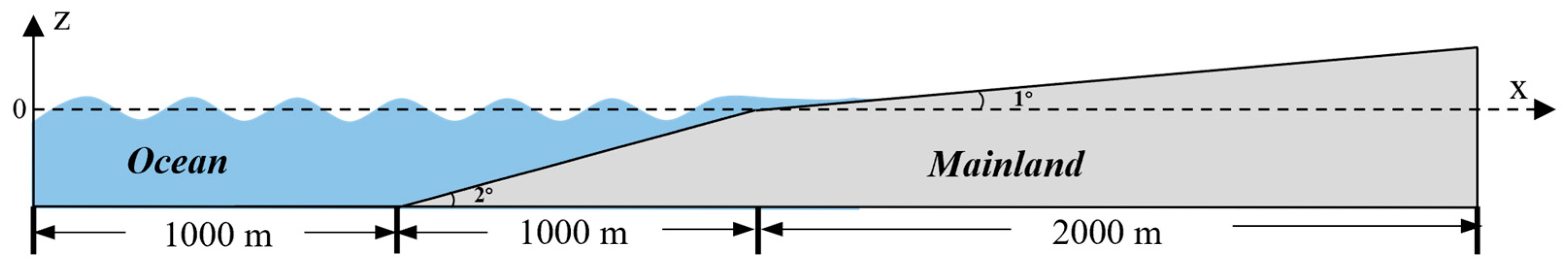
3.1. Test Setup
3.2. Results
3.3. Adaptive LTS Method
- (1)
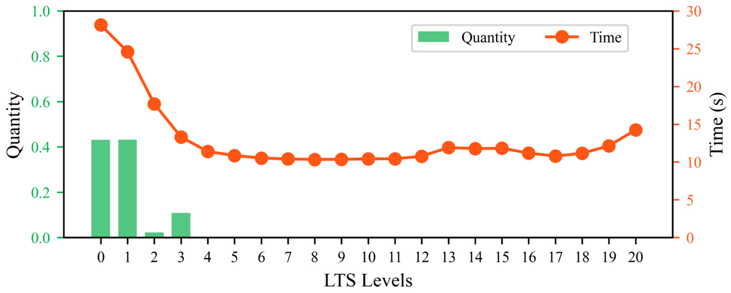
- Model without dry cells: In this case, the model contained no dry cells, and the computational process was stable with an even distribution of computational load across cells. Experimental results indicate that, in this case, the optimal LTS level can directly adopt the , meaning the optimal level is identical to the under quiescent water conditions.
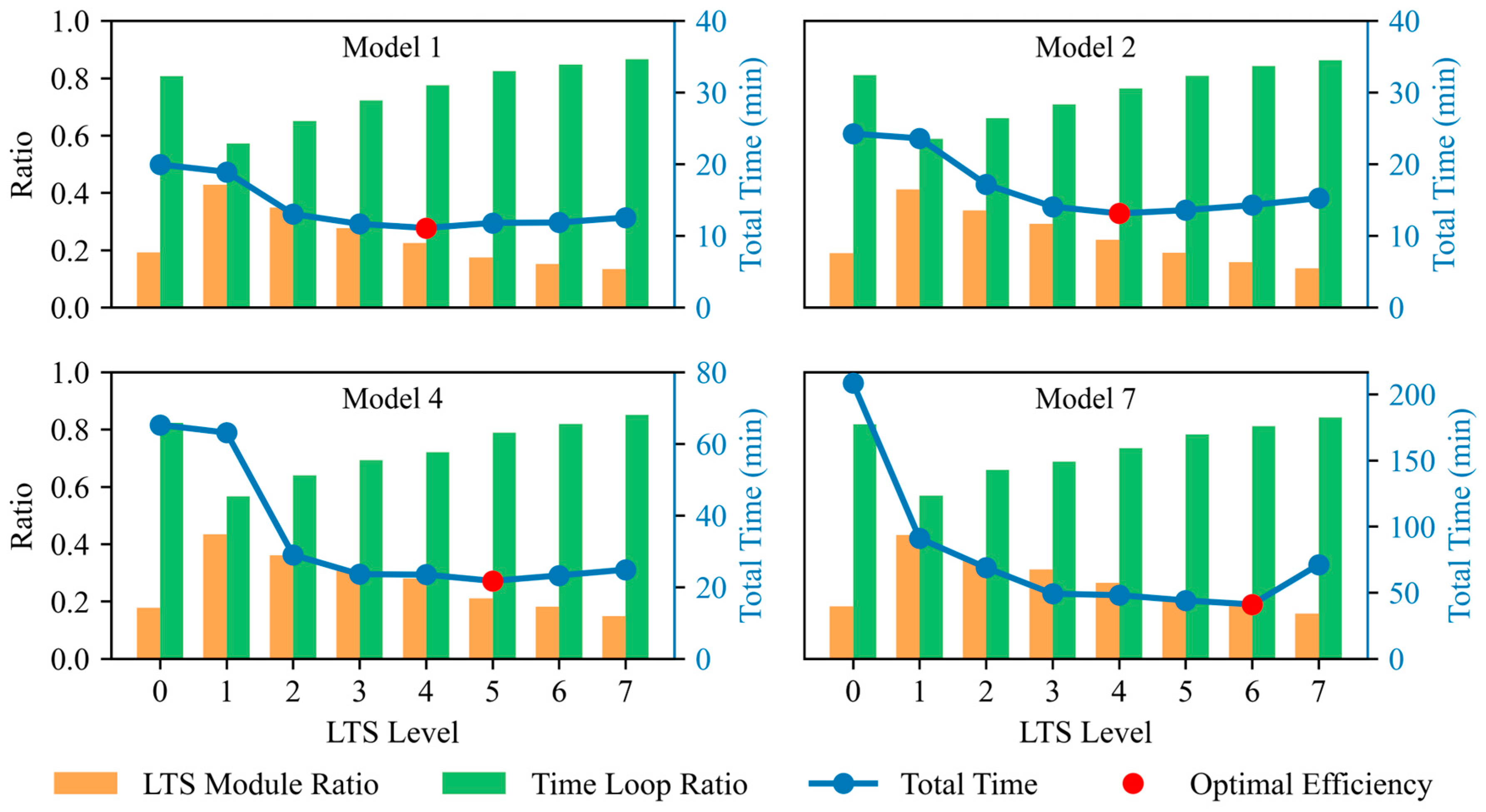
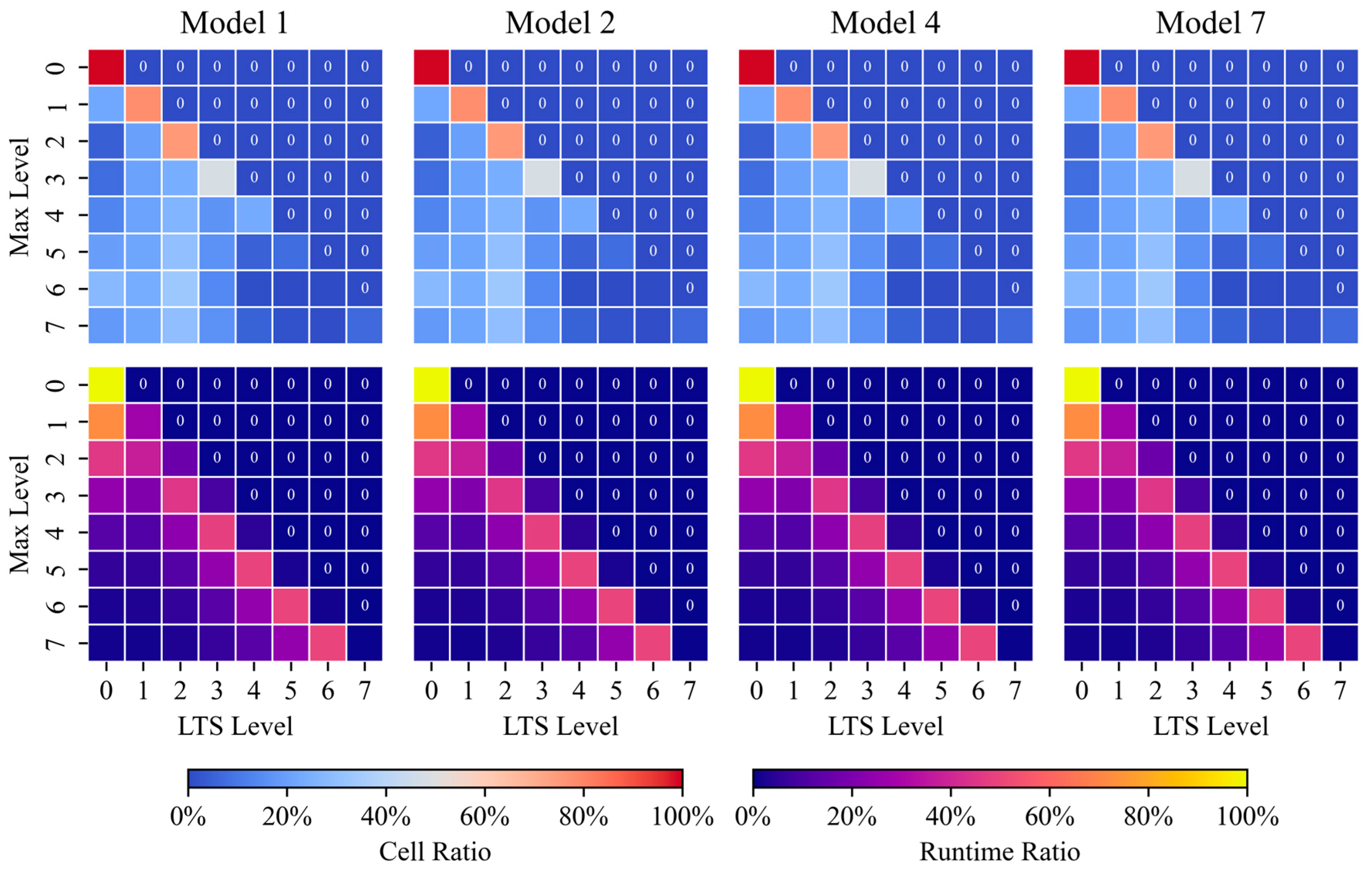
- (2)
- Model with dry cells: In the presence of dry cells, frequent changes at the dry–wet interface significantly increase computational complexity and instability. Therefore, we dynamically adjusted based on the dry cell ratio (). Through extensive experimental data analysis, we modeled this adjustment as a piecewise function (Equation (29)), with breakpoints set at and , with the following rules: when the is between 30 and 50%, increases by one level from , i.e., ; when is between 60 and 80%, increases by two levels from , i.e., . To maintain consistency across different models, we adopted conservative critical values of and in all experiments in this study. Finally, considering the impact of frequent changes at the dry–wet interface on computational stability and efficiency, the experiments revealed that when exceeds 7, the improvement in computational efficiency diminishes and may even introduce additional computational overhead. Therefore, it is not recommended to set above 7.
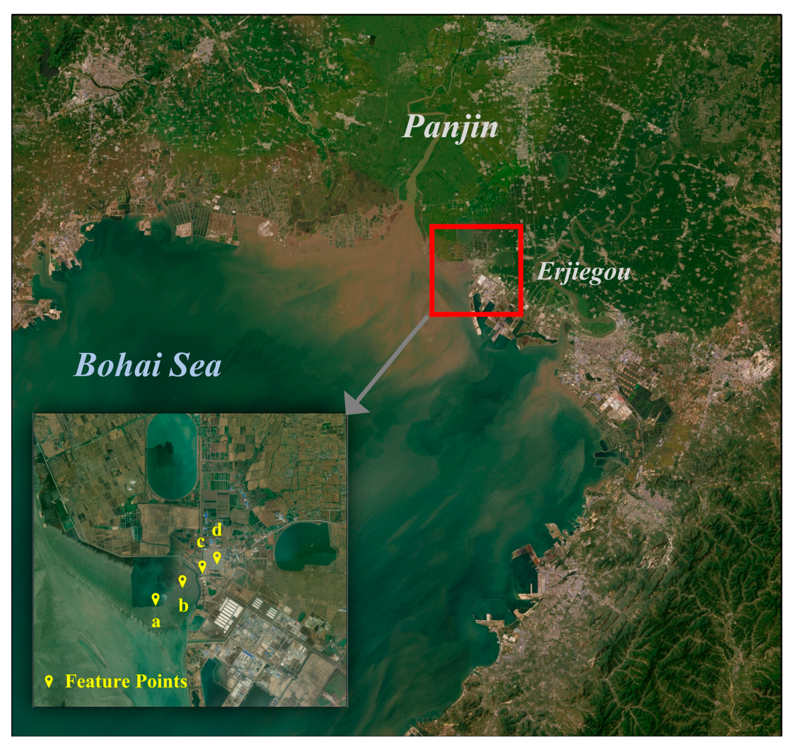
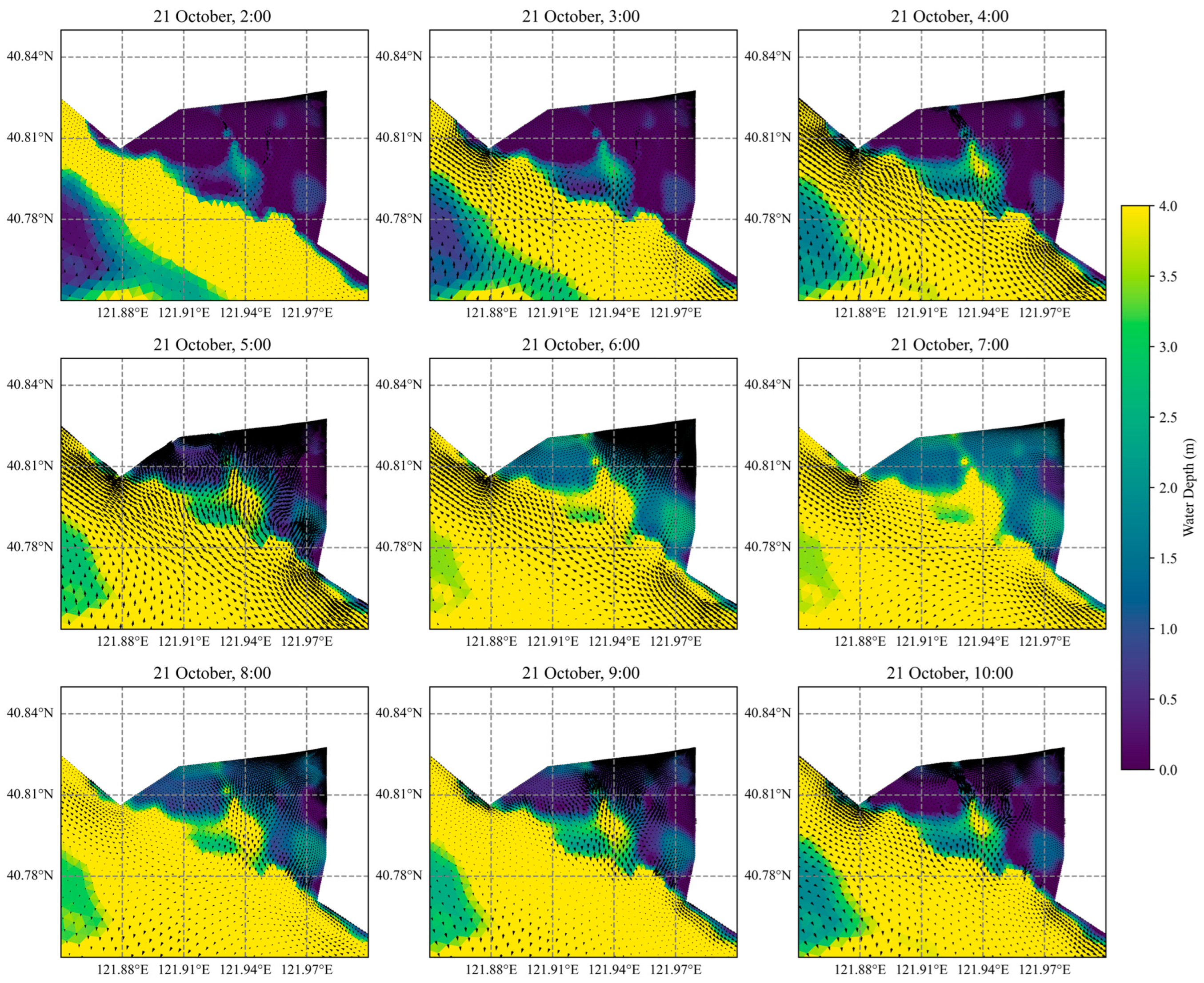
4. Application to Simulating Storm Surge Inundation in a Complex Coastal Area
5. Conclusions
6. Discussion
Author Contributions
Funding
Institutional Review Board Statement
Informed Consent Statement
Data Availability Statement
Conflicts of Interest
References
- Liu, G.; Yang, W.; Jiang, Y.; Yin, J.; Tian, Y.; Wang, L.; Xu, Y. Design Wave Height Estimation under the Influence of Typhoon Frequency, Distance, and Intensity. J. Mar. Sci. Eng. 2023, 11, 1712. [Google Scholar] [CrossRef]
- Liu, G.; Yang, B.; Nong, X.; Kou, Y.; Wu, F.; Zhao, D.; Yu, P. Risk Level Assessment of Typhoon Hazard Based on Loss Utility. J. Mar. Sci. Eng. 2023, 11, 2177. [Google Scholar] [CrossRef]
- Zhu, Z.; Wang, Z.; Dong, C.; Yu, M.; Xie, H.; Cao, X.; Han, L.; Qi, J. Physics Informed Neural Network Modelling for Storm Surge Forecasting—A Case Study in the Bohai Sea, China. Coast. Eng. 2025, 197, 104686. [Google Scholar] [CrossRef]
- Wang, Z.; Chen, Y.; Zeng, Z.; Li, R.; Li, Z.; Li, X.; Lai, C. Compound Effects in Complex Estuary-Ocean Interaction Region under Various Combination Patterns of Storm Surge and Fluvial Floods. Urban Clim. 2024, 58, 102186. [Google Scholar] [CrossRef]
- Zhang, J.; Wu, G.; Liang, B.; Shi, L. Modeling Wave Attenuation through Vegetation Patches: The Overlooked Role of Spatial Heterogeneity. Phys. Fluids 2024, 36, 077102. [Google Scholar] [CrossRef]
- Zhuge, W.; Wu, G.; Liang, B.; Yuan, Z.; Zheng, P.; Wang, J.; Shi, L. A Statistical Method to Quantify the Tide-Surge Interaction Effects with Application in Probabilistic Prediction of Extreme Storm Tides along the Northern Coasts of the South China Sea. Ocean Eng. 2024, 298, 117151. [Google Scholar] [CrossRef]
- Tomasicchio, G.R.; Salvadori, G.; Lusito, L.; Francone, A.; Saponieri, A.; Leone, E.; De Bartolo, S. A Statistical Analysis of the Occurrences of Critical Waves and Water Levels for the Management of the Operativity of the MoSE System in the Venice Lagoon. Stoch. Environ. Res. Risk Assess. 2022, 36, 2549–2560. [Google Scholar] [CrossRef]
- Wang, K.; Wu, G.; Liang, B.; Shi, B.; Li, H. Linking Marsh Sustainability to Event-Based Sedimentary Processes: Impulsive River Floods Initiated Lateral Erosion of Deltaic Marshes. Coast. Eng. 2024, 190, 104515. [Google Scholar] [CrossRef]
- Wang, K.; Wu, G.; Liang, B.; Shi, B.; Li, H. Deltaic Marsh Accretion under Episodic Sediment Supply Controlled by River Regulations and Storms: Implications for Coastal Wetlands Restoration in the Yellow River Delta. J. Hydrol. 2024, 635, 131221. [Google Scholar] [CrossRef]
- Carlotto, T.; Chaffe, P.L.B.; dos Santos, C.I.; Lee, S. SW2D-GPU: A Two-Dimensional Shallow Water Model Accelerated by GPGPU. Environ. Model. Softw. 2021, 145, 105205. [Google Scholar] [CrossRef]
- Dazzi, S.; Vacondio, R.; Dal Palù, A.; Mignosa, P. A Local Time Stepping Algorithm for GPU-Accelerated 2D Shallow Water Models. Adv. Water Resour. 2018, 111, 274–288. [Google Scholar]
- Hu, P.; Zhao, Z.X.; Ji, A.F.; Li, W.; He, Z.G.; Liu, Q.F.; Li, Y.W.; Cao, Z.X. A GPU-Accelerated and LTS-Based Finite Volume Shallow Water Model. Water 2022, 14, 922. [Google Scholar] [CrossRef]
- Osher, S.; Sanders, R. Numerical Approximations to Nonlinear Conservation Laws with Locally Varying Time and Space Grids. Math. Comput. 1983, 41, 321–336. [Google Scholar]
- Dawson, C. High Resolution Upwind-Mixed Finite Element Methods for Advection-Diffusion Equations with Variable Time-Stepping. Numer. Methods Partial Differ. Equ. 1995, 11, 525–538. [Google Scholar]
- Dawson, C.; Kirby, R. High Resolution Schemes for Conservation Laws with Locally Varying Time Steps. SIAM J. Sci. Comput. 2001, 22, 2256–2281. [Google Scholar]
- Dawson, C. A Local Timestepping Runge–Kutta Discontinuous Galerkin Method for Hurricane Storm Surge Modeling. In Recent Developments in Discontinuous Galerkin Finite Element Methods for Partial Differential Equations; Feng, X., Karakashian, O., Xing, Y., Eds.; Springer International Publishing: Cham, Switzerland, 2014; Volume 157, pp. 133–148. ISBN 978-3-319-01817-1. [Google Scholar]
- Dawson, C.; Trahan, C.J.; Kubatko, E.J.; Westerink, J.J. A Parallel Local Timestepping Runge–Kutta Discontinuous Galerkin Method with Applications to Coastal Ocean Modeling. Comput. Methods Appl. Mech. Eng. 2013, 259, 154–165. [Google Scholar]
- Crossley, A.J.; Wright, N.G. Time Accurate Local Time Stepping for the Unsteady Shallow Water Equations. Int. J. Numer. Methods Fluids 2005, 48, 775–799. [Google Scholar]
- Crossley, A.J.; Wright, N.G.; Whitlow, C.D. Local Time Stepping for Modeling Open Channel Flows. J. Hydraul. Eng. 2003, 129, 455–462. [Google Scholar]
- Krámer, T.; Józsa, J. Solution-Adaptivity in Modelling Complex Shallow Flows. Comput. Fluids 2007, 36, 562–577. [Google Scholar]
- Tan, Z.J.; Zhang, Z.R.; Huang, Y.Q.; Tang, T. Moving Mesh Methods with Locally Varying Time Steps. J. Comput. Phys. 2004, 200, 347–367. [Google Scholar]
- Sanders, B.F. Integration of a Shallow Water Model with a Local Time Step. J. Hydraul. Res. 2008, 46, 466–475. [Google Scholar]
- Yang, X.; An, W.; Li, W.; Zhang, S. Implementation of a Local Time Stepping Algorithm and Its Acceleration Effect on Two-Dimensional Hydrodynamic Models. Water 2020, 12, 1148. [Google Scholar] [CrossRef]
- Hu, P.; Lei, Y.L.; Han, J.J.; Cao, Z.X.; Liu, H.H.; He, Z.G. Computationally Efficient Modeling of Hydro-Sediment-Morphodynamic Processes Using a Hybrid Local Time Step/Global Maximum Time Step. Adv. Water Resour. 2019, 127, 26–38. [Google Scholar]
- Hu, P.; Lei, Y.; Han, J.; Cao, Z.; Liu, H.; He, Z.; Yue, Z. Improved Local Time Step for 2D Shallow-Water Modeling Based on Unstructured Grids. J. Hydraul. Eng. 2019, 145, 06019017.1–06019017.9. [Google Scholar]
- Wu, J.; Hu, P.; Zhao, Z.; Lin, Y.-T.; He, Z. A GPU-Accelerated and LTS-Based 2D Hydrodynamic Model for the Simulation of Rainfall-Runoff Processes. J. Hydrol. 2023, 623, 129735. [Google Scholar] [CrossRef]
- Zhao, Z.; Hu, P.; Li, W.; Cao, Z.; Li, Y. An Engineering-Oriented Shallow-Water Hydro-Sediment-Morphodynamic Model Using the GPU-Acceleration and the Hybrid LTS/GMaTS Method. Adv. Eng. Softw. 2025, 200, 103821. [Google Scholar] [CrossRef]
- Hoang, T.-T.-P.; Leng, W.; Ju, L.L.; Wang, Z.; Pieper, K. Conservative Explicit Local Time-Stepping Schemes for the Shallow Water Equations. J. Comput. Phys. 2019, 382, 152–176. [Google Scholar]
- Capodaglio, G.; Petersen, M. Local Time Stepping for the Shallow Water Equations in MPAS. J. Comput. Phys. 2022, 449, 110818. [Google Scholar] [CrossRef]
- Lilly, J.R.; Capodaglio, G.; Petersen, M.R.; Brus, S.R.; Engwirda, D.; Higdon, R.L. Storm Surge Modeling as an Application of Local Time-Stepping in MPAS-Ocean. J. Adv. Model. Earth Syst. 2023, 15, e2022MS003327. [Google Scholar]
- Liu, G.; Ji, T.; Wu, G.; Yu, P. Improved Local Time-Stepping Schemes for Storm Surge Modeling on Unstructured Grids. Environ. Model. Softw. 2024, 179, 106107. [Google Scholar] [CrossRef]
- Liu, G.; Ji, T.; Wu, G.; Tian, H.; Yu, P. Cross-Scale Modeling of Shallow Water Flows in Coastal Areas with an Improved Local Time-Stepping Method. J. Mar. Sci. Eng. 2024, 12, 1065. [Google Scholar] [CrossRef]
- Toro, E.F. Riemann Solvers and Numerical Methods for Fluid Dynamics; Springer: Berlin/Heidelberg, Germany, 2013. [Google Scholar]
- Yu, P.B.; Pan, C.H.; Xie, Y.L. 2-Dimensional Real Time Forecasting Model for Storm Tides and Its Application in Hangzhou Bay. J. Hydrodynomics 2011, 26, 747–756. [Google Scholar]
- Huang, S.; Xu, J.; Wang, D.; Lu, D. Variation Assimilation Model of Storm Surge. Chin. J. Hydrodyn. 2010, 4, 469–474. [Google Scholar]
- Egbert, G.D.; Erofeeva, S.Y. Efficient Inverse Modeling of Barotropic Ocean Tides. J. Atmos. Ocean. Technol. 2002, 19, 183–204. [Google Scholar] [CrossRef]
- Hersbach, H.; Bell, B.; Berrisford, P.; Hirahara, S.; Horányi, A.; Muñoz-Sabater, J.; Nicolas, J.; Peubey, C.; Radu, R.; Schepers, D.; et al. The ERA5 Global Reanalysis. Q. J. R. Meteorol. Soc. 2020, 146, 1999–2049. [Google Scholar] [CrossRef]


| Model | 1 | 2 | 3 | 4 | 5 | 6 | 7 | 8 |
|---|---|---|---|---|---|---|---|---|
| Number of nodes | 6425 | 8278 | 9381 | 14,934 | 16,606 | 18,799 | 26,532 | 50,221 |
| Number of cells | 12,624 | 16,282 | 18,463 | 29,467 | 32,785 | 37,139 | 52,506 | 99,648 |
| Proportion of dry cells | 35% | 42% | 46% | 58% | 60% | 64% | 71% | 82% |
| Maximum level () | 7 | 7 | 7 | 7 | 7 | 7 | 7 | 7 |
| Optimal efficiency level | 4 | 4 | 5 | 5 | 5 | 5 | 6 | 6 |
| Speedup | 1.71 | 1.79 | 2.12 | 3.00 | 3.34 | 3.58 | 5.02 | 5.69 |
| Model | 1 | 2 | 3 | 4 | 5 | 6 | 7 | 8 |
|---|---|---|---|---|---|---|---|---|
| Minimum Level | 4 | 4 | 4 | 4 | 4 | 4 | 4 | 4 |
| Maximum Level | 5 | 6 | 6 | 6 | 6 | 6 | 6 | 6 |
| Vs. GTS | 1.83 | 1.87 | 2.71 | 3.16 | 3.66 | 3.51 | 5.30 | 5.83 |
| Vs. | +0.12 | +0.08 | +0.59 | +0.16 | +0.32 | −0.07 | +0.28 | +0.12 |
| Model | Tidal Flow Process | Storm Surge Process1 | Storm Surge Process2 |
|---|---|---|---|
| GTS Time (h) | 58.36 | 18.65 | 18.13 |
| Optimal Limit Level () | 7 | 7 | 7 |
| Limit Level Time (h) | 9.58 | 3.32 | 3.27 |
| Speedup | 6.09 | 5.62 | 5.54 |
| Adaptive Method Time (h) | 9.03 | 3.29 | 3.18 |
| Speedup | 6.46 | 5.67 | 5.70 |
| Speedup Difference | +0.37 | +0.05 | +0.16 |
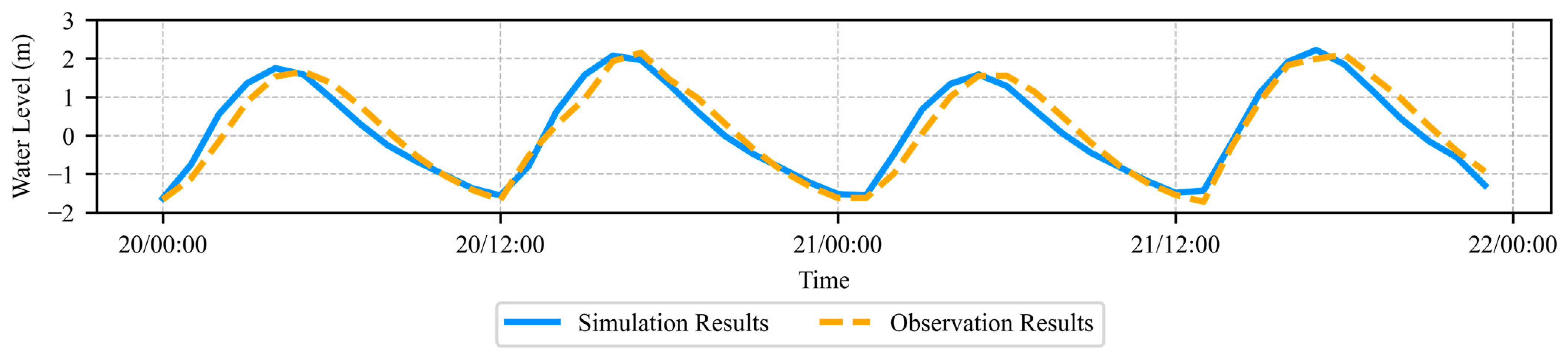
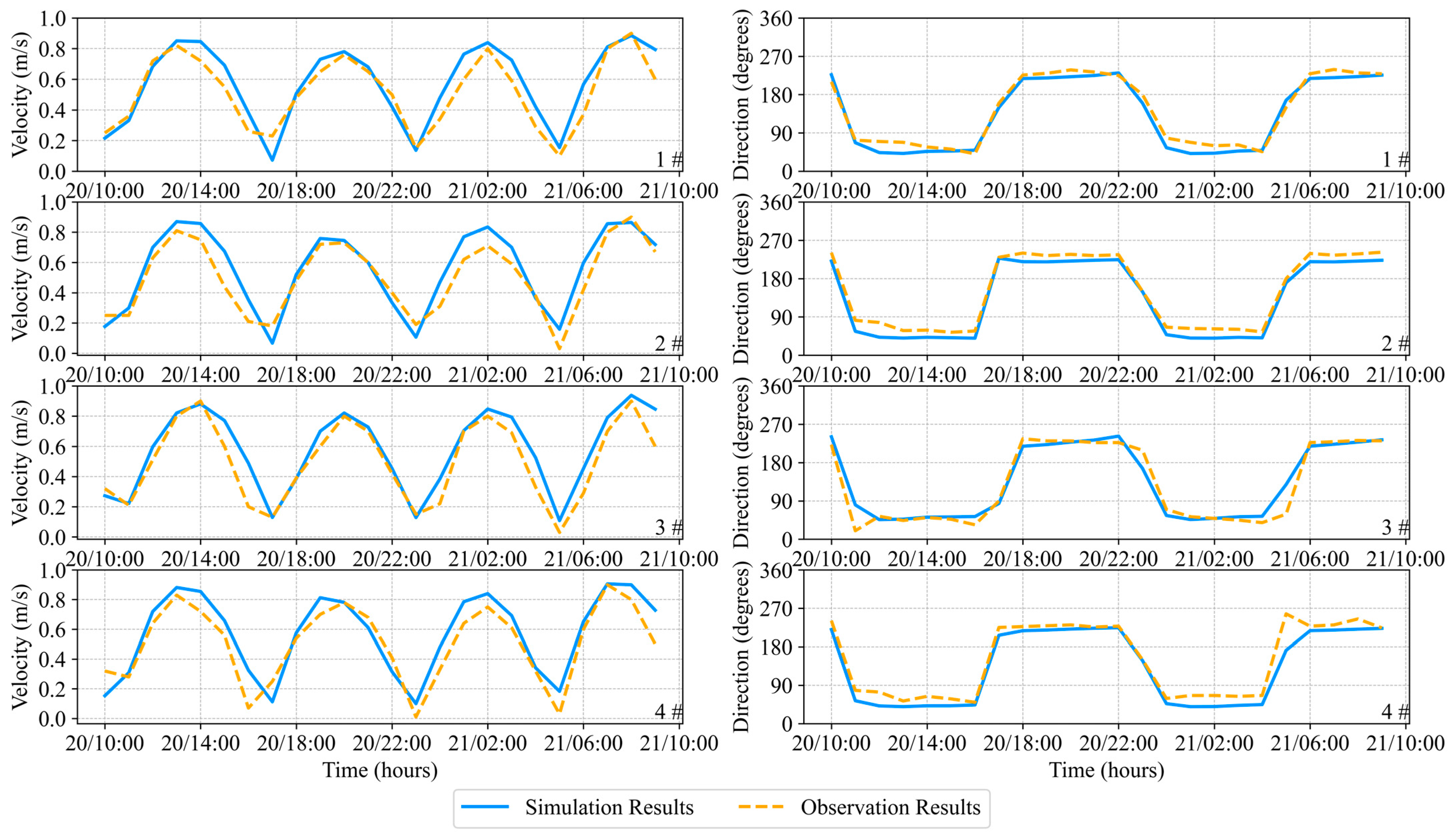
| Water Level | 1# Velocity | 1# Direction | 2# Velocity | 2# Direction | 3# Velocity | 3# Direction | 4# Velocity | 4# Direction | |
|---|---|---|---|---|---|---|---|---|---|
| RMSE | 0.31 | 0.10 | 15.15 | 0.10 | 17.83 | 0.11 | 22.83 | 0.11 | 24.32 |
| MAE | 0.25 | 0.08 | 13.36 | 0.09 | 16.48 | 0.08 | 14.55 | 0.10 | 18.00 |
| Skill Score | 0.93 | 0.79 | 0.96 | 0.80 | 0.95 | 0.81 | 0.93 | 0.78 | 0.91 |
Disclaimer/Publisher’s Note: The statements, opinions and data contained in all publications are solely those of the individual author(s) and contributor(s) and not of MDPI and/or the editor(s). MDPI and/or the editor(s) disclaim responsibility for any injury to people or property resulting from any ideas, methods, instructions or products referred to in the content. |
© 2025 by the authors. Licensee MDPI, Basel, Switzerland. This article is an open access article distributed under the terms and conditions of the Creative Commons Attribution (CC BY) license (https://creativecommons.org/licenses/by/4.0/).
Share and Cite
Yu, P.; Ji, T.; Wu, X.; Chen, Y.; Liu, G. An Adaptive Local Time-Stepping Method Applied to Storm Surge Inundation Simulation. J. Mar. Sci. Eng. 2025, 13, 467. https://doi.org/10.3390/jmse13030467
Yu P, Ji T, Wu X, Chen Y, Liu G. An Adaptive Local Time-Stepping Method Applied to Storm Surge Inundation Simulation. Journal of Marine Science and Engineering. 2025; 13(3):467. https://doi.org/10.3390/jmse13030467
Chicago/Turabian StyleYu, Pubing, Tao Ji, Xiuguang Wu, Yifan Chen, and Guilin Liu. 2025. "An Adaptive Local Time-Stepping Method Applied to Storm Surge Inundation Simulation" Journal of Marine Science and Engineering 13, no. 3: 467. https://doi.org/10.3390/jmse13030467
APA StyleYu, P., Ji, T., Wu, X., Chen, Y., & Liu, G. (2025). An Adaptive Local Time-Stepping Method Applied to Storm Surge Inundation Simulation. Journal of Marine Science and Engineering, 13(3), 467. https://doi.org/10.3390/jmse13030467