Numerical and Experimental Study of a Hydrodynamic Analysis of the Periodical Fluctuation of Bio-Inspired Banded Fins

Abstract

A bio-inspired vehicle with banded fin fluctuation as the propulsion mode is the research topic. However, this propulsion mode suffers from low efficiency and requires the urgent resolution of other issues. In this paper, the kinematic model of the banded fin surface and the numerical calculation model for its hydrodynamic performance are established based on the long dorsal fin propelled by MPF (Media and/or Paired Fin propulsion) mode. Through numerical simulation, the hydrodynamic performance of the banded fin under typical working conditions is explored and its propulsion mechanism is analyzed. By using a method of controlling variables, such as wave number, swing angle, and frequency, where only one independent variable is changed at a time while the others remain constant, the impact on thrust coefficient function and the obtained periodic variation laws governing hydrodynamic performance are studied. Oscillatory thrust is generated by the fin’s motion, where it first captures water through a ‘scoop’ motion and then expels it via a diagonal ‘push’ motion, producing thrust. Due to limitations in fin length and varying oscillation shapes, the effective water-pushing stroke differs, leading to variations in work and creating periodic oscillatory forces. When the variable is the oscillation frequency, the propulsion efficiency of the oscillating fins remains nearly constant when the oscillation frequency is less than or equal to 1 Hz. However, when the oscillation frequency exceeds 1 Hz, the propulsion efficiency decreases as the oscillation frequency increases, and the rate of decrease gradually slows down. The effect of leading-edge suction on hydrodynamic performance was studied by varying the oscillating fin’s angle of attack. The results showed that, compared to the unchamfered configuration, the forward chamfer better utilizes vortex energy, reducing input power and significantly improving propulsion efficiency. Guided by both numerical simulations and experimental results, we design and manufacture a prototype of an underwater banded fin bio-inspired propeller that encompasses shape modeling, mechanical structure design, and control mechanism design. We conduct real water tests to verify feasibility and reliability in terms of forward movement, backward movement, and turning ability, among others. Furthermore, we analyze how varying angle of attack or optimizing front/rear edge shapes can effectively enhance hydrodynamic performance.

1. Introduction

Currently, fish-like vehicles employ two primary propulsion modes: BCF (Body and/or Caudal Fin propulsion) and MPF (Media and/or Paired Fin propulsion). In natural environments, approximately 15% of fish species utilize the MPF mode as their main means of propulsion, relying on dorsal, pectoral, and pelvic fins (Breder [1]; Webb and Paul [2]). In comparison to the BCF mode, this particular mode exhibits evident advantages in terms of stability and maneuverability at low speeds: the underwater vehicle, propelled by the MPF mode, incorporates bionic wave fins on both sides that generate turning torque through asymmetric movement and other mechanisms to enable turning motion. Additionally, reverse transmission of traveling waves facilitates reversing, thereby enhancing the maneuverability of underwater vehicles. By adjusting the angle of attack of fluctuating fins using a steering gear, heave and pitch motions can be achieved with strong maneuverability. The inclusion of low-disturbance floating fins ensures stealthy performance while wave propulsion eliminates interference from debris such as water grass or reed, exhibiting excellent environmental adaptability. Furthermore, by utilizing ground friction during contact between wave fin crests and surfaces, beaching, as well as walking on land or snow, can be accomplished effectively, showcasing remarkable amphibious capabilities. Hence, it serves as an exceptional operational platform for specialized tasks such as underwater detection and reconnaissance.

In light of this, both domestic and foreign scholars have conducted comprehensive studies on the propulsion mechanism, hydrodynamic performance, and optimization strategy of banded fins in MPF propulsion mode. Lighthill [3] introduced the “slender body theory” from aerodynamics into hydrodynamics for the first time. He simplified fish bodies as slender bodies and further proposed the “large swing slender body theory”. Lighthill [4] provided an analytical solution for swimming efficiency based on potential flow theory (Lighthill [5]). Cheng et al. [6] and Tong et al. [7] assumed rectangular or triangular thin plates to represent fish bodies and developed the Three-dimensional Undulating Plate Theory (3DWPT). By combining linearized boundary conditions with a plane wake model, they employed the unsteady vortex lattice method derived from potential flow theory to investigate how parameters related to a fish’s swimming propulsion wave and fin shape influence its propulsion performance. This theory has gained wide acceptance among international counterparts and is extensively used in analyzing the hydrodynamic characteristics of banded fins (Cheng and Blickhan [8]; Mchenry et al. [9]; Pedley and Hill [10]; Miriam [11]; Long et al. [12]). Zhang [13] focused his research on studying the propulsion performance of banded fins. Through comparing two fluctuation modes—constant amplitude from front to back versus gradually changing amplitude from front to back—he concluded that maintaining a constant amplitude yields better propulsion performance and swimming stability. Zhang [14] and Liu [15] optimized and evaluated the hydrodynamic performance of banded fins by considering morphology and function using the equations governing the control of unsteady 3D flow along with neural network techniques. Their work provides valuable guidance for the further analysis of banded fin fluctuation’s propulsion mechanism, as well as research aimed at enhancing its overall performance. Zhang et al. [16] investigated the contribution of vortices at various positions to the hydrodynamic performance of banded fins by analyzing the vorticity field. They proposed a method for balancing local structural effects and overall fin performance through moderate chordwise deformation of the fin surface, providing new insights into the role of vortices in underwater motion and force enhancement mechanisms. Simultaneously, a bio-inspired underwater vehicle with banded-like fins can be manufactured to fulfill the requirements of low-speed operations, drawing inspiration from the flapping mechanism of flexible fins. Zhou et al. [17] conducted computational fluid dynamics simulations and experimental comparisons to reveal specific phenomena in the bio-inspired flapping mode. Zeng et al. [18] integrated wave fins with quadrotors, establishing dynamic equations for underwater motion and conducting experimental verification. He et al. [19] and Xing et al. [20] investigated batfish, designing and manufacturing bio-inspired underwater vehicles that imitate batfish and enhance their underwater navigation performance through a novel pectoral fin mechanical structure. Wei et al. [21] numerically simulated the convective fin system based on the high-resolution numerical technique of the constrained immersion boundary method, and revealed the basic variation law between the hydrodynamic performance and motion parameters of the fluctuating fin. Shi et al. [22] used the ghost cell method to study the fluid dynamics of three-dimensional fish swimming in oblique flow. Chen et al. [23] conducted research on the underwater motion modeling and closed-loop control of a bionic undulating fin robot, enhancing the control accuracy and stability by establishing a dynamic model and developing a neural network PID controller. Li et al. [24] proposed a separated undulating fin propulsion method to enhance thrust, achieving up to 13.5% greater thrust compared to traditional fins, and revealed the underlying mechanisms through numerical simulations and fluid dynamics experiments. Li et al. [25] developed a separated undulating fins model inspired by dragonflies to improve thrust stability for underwater robots, demonstrating through numerical simulation and experimental validation that this approach can significantly reduce thrust fluctuations and enhance control precision. Shi et al. [26] investigated the hydrodynamic performance of 2D undulating fins in the wake of a semi-cylinder using numerical simulation, revealing the impact of varying flow conditions on fin propulsion and providing insights into the passive hydrodynamic interactions of fins. Sun et al. [27] conducted a numerical study on the propulsive efficiency of an undulating fin propulsor, finding that increasing amplitude decreases efficiency and that higher frequencies improve stability, offering valuable insights for the shape optimization of undulating fins. Vu et al. [28] developed a swimming mode controller for an elongated undulating fin robot using multi-agent deep deterministic policy gradient (MA-DDPG), achieving superior propulsive efficiency compared to traditional reinforcement learning methods. Wei et al. [29] analyzed the hydrodynamic performance of dual three-dimensional undulating fin formations, revealing that side-by-side arrangements reduce thrust and energy consumption, while tandem formations enhance rear fin thrust but increase energy use, providing insights into the collective behaviors of undulating fins. Xia et al. [30] introduced a novel IB-LB method for predicting the hydrodynamics of bionic undulating fin thrusters (BUFTs), demonstrating increased propulsive force and efficiency with higher Reynolds numbers and optimizing propulsion performance at specific frequency and amplitude conditions. Yu et al. [31,32] proposed a novel design with separated elastic fin rays and asynchronous control for undulating fin amphibious robots to enhance terrestrial locomotion stability, demonstrating significant improvements in postural stability through both simulation and experimental validation.

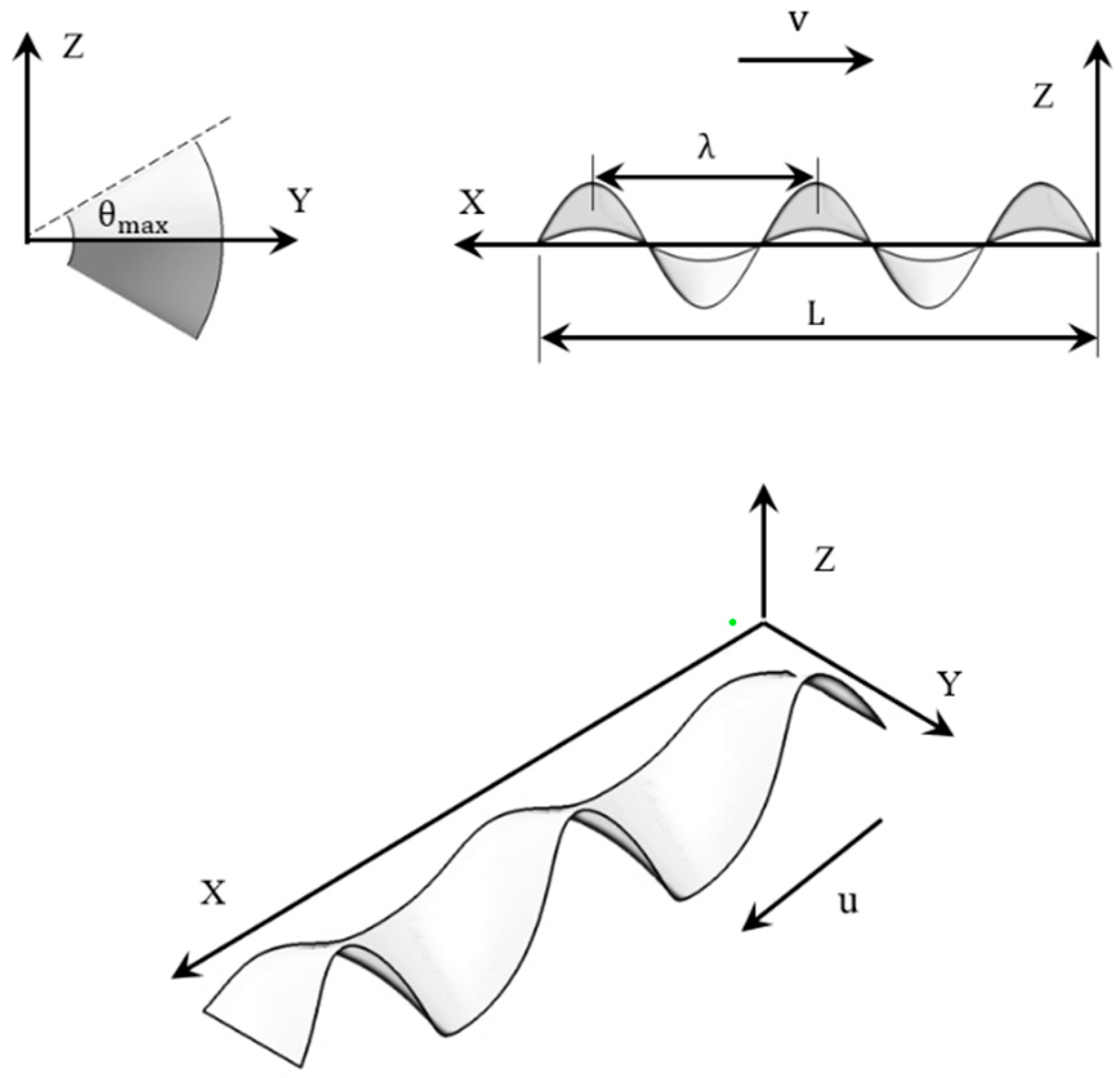
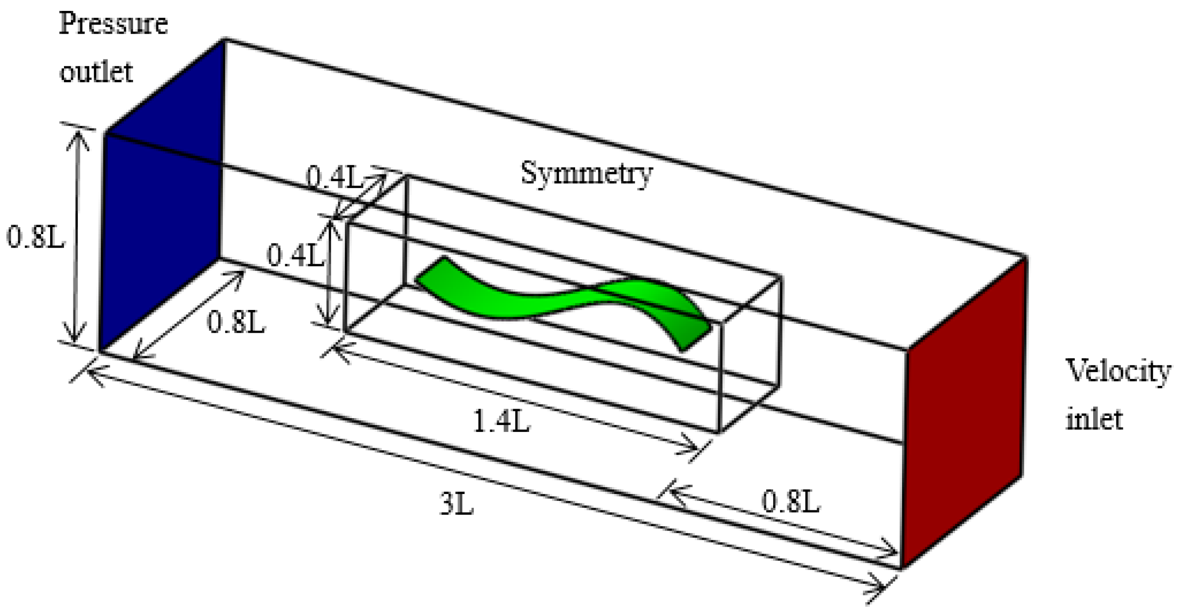
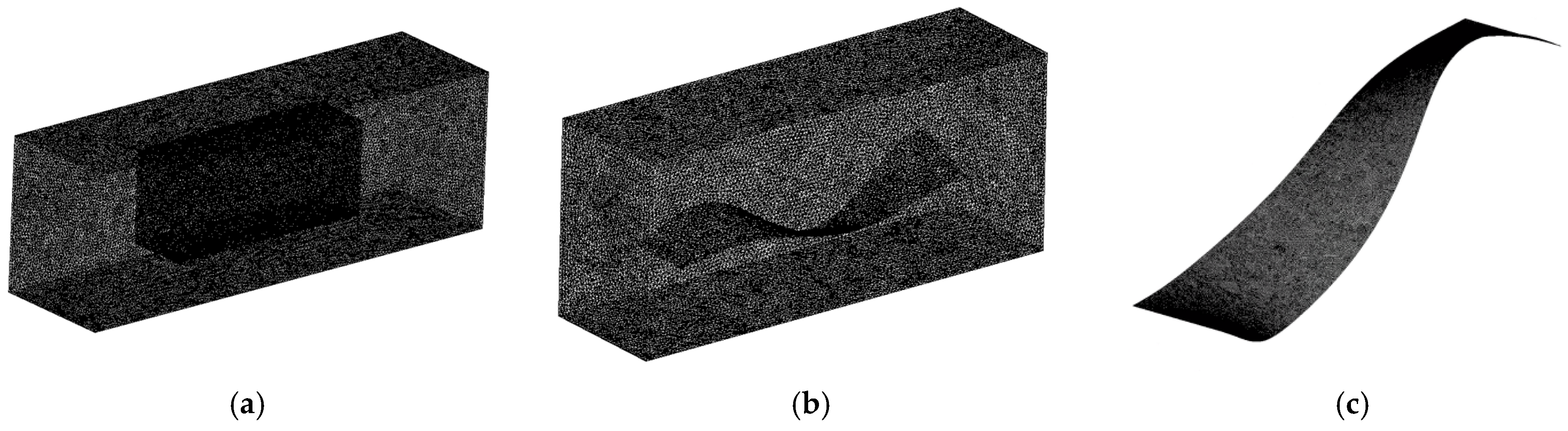
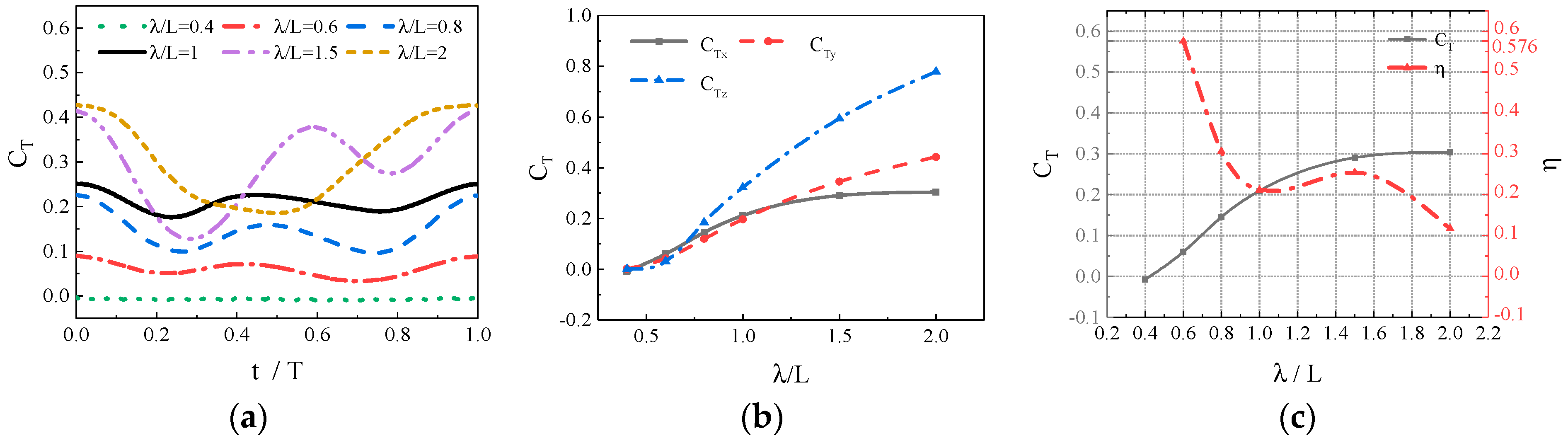
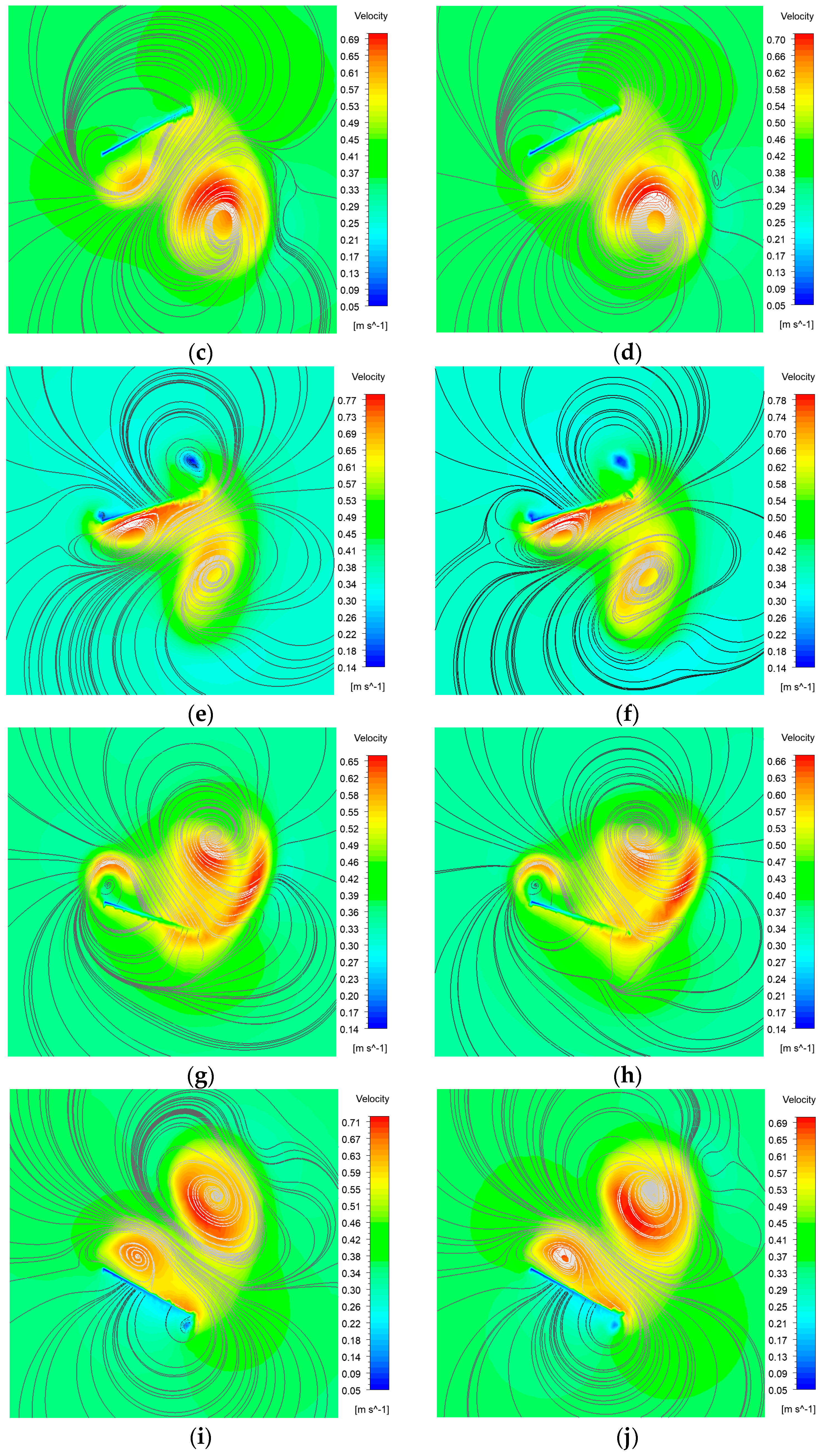
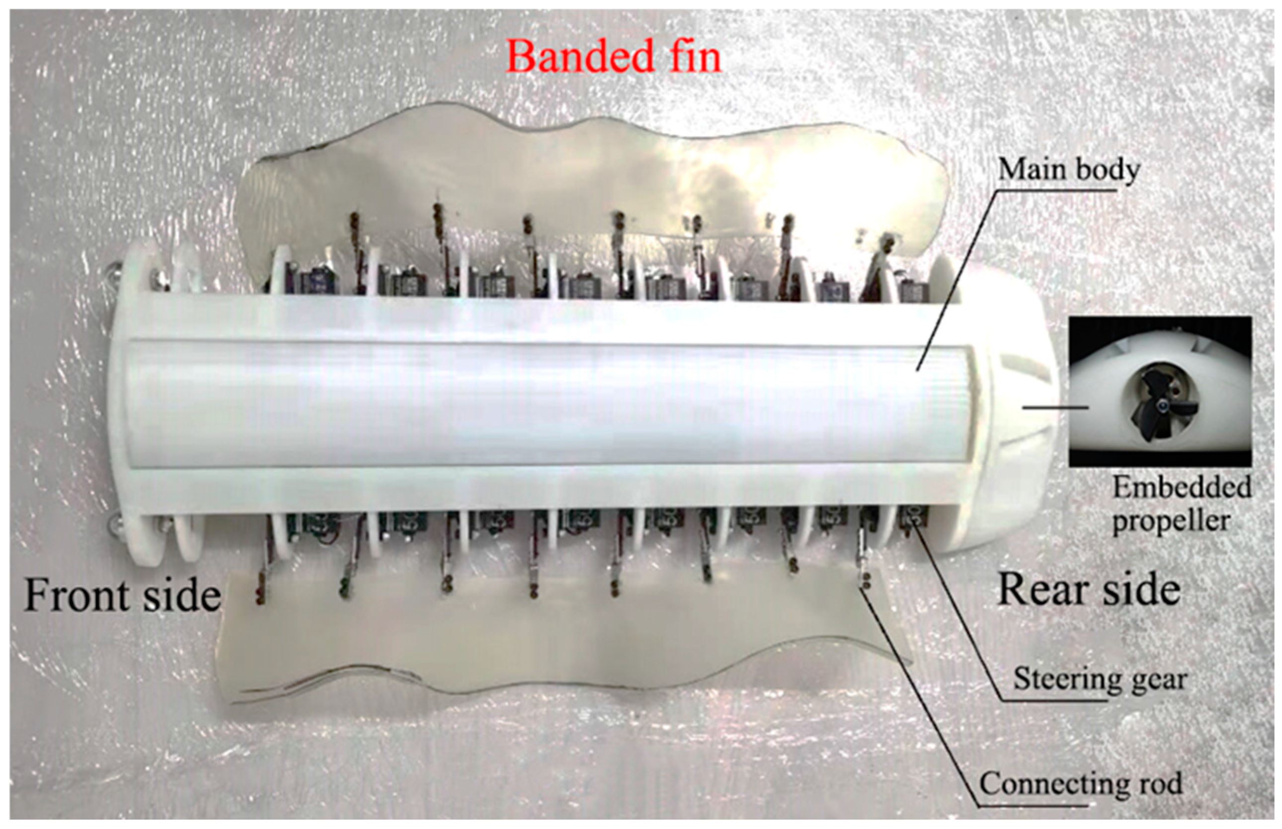
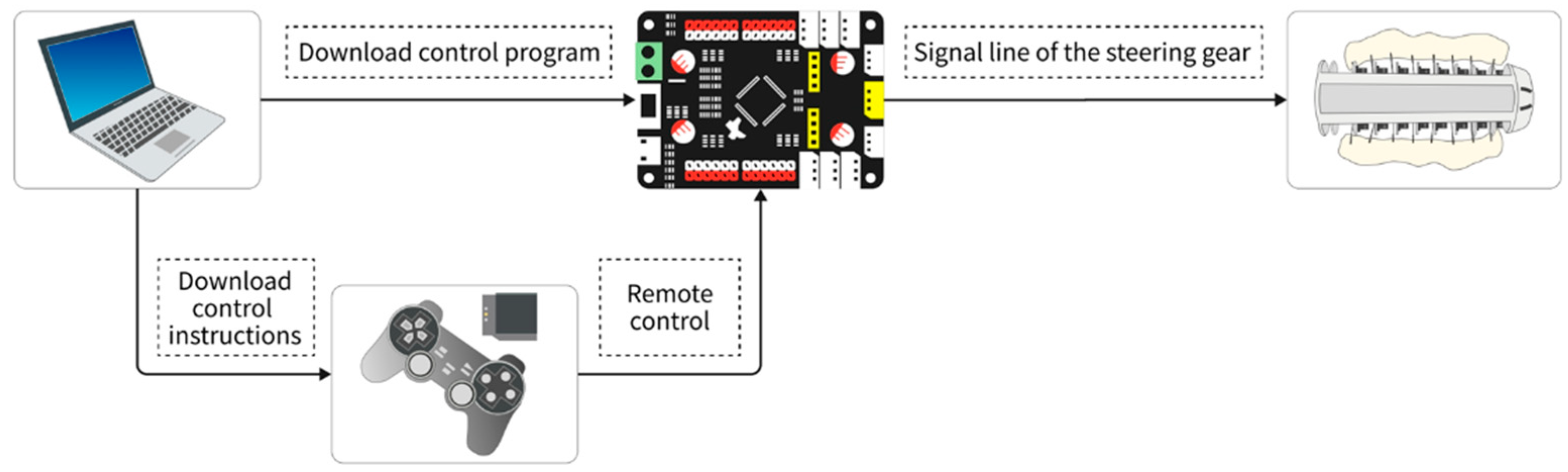
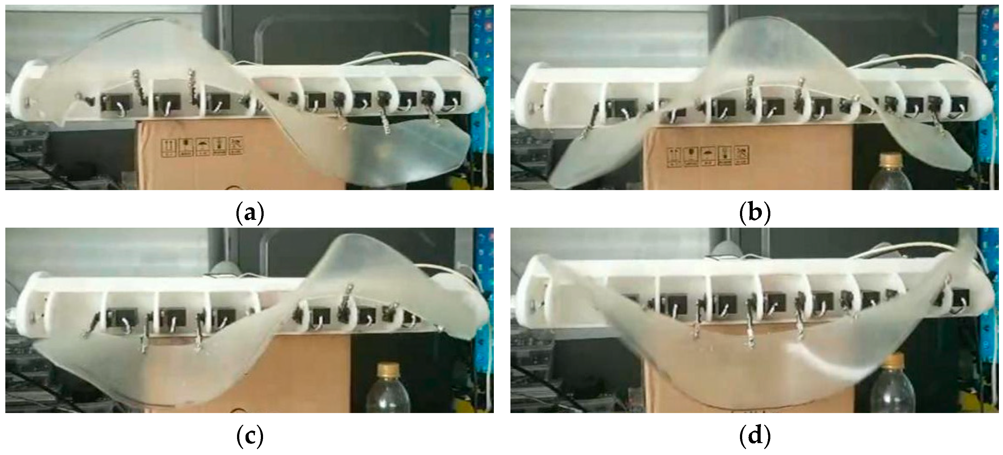
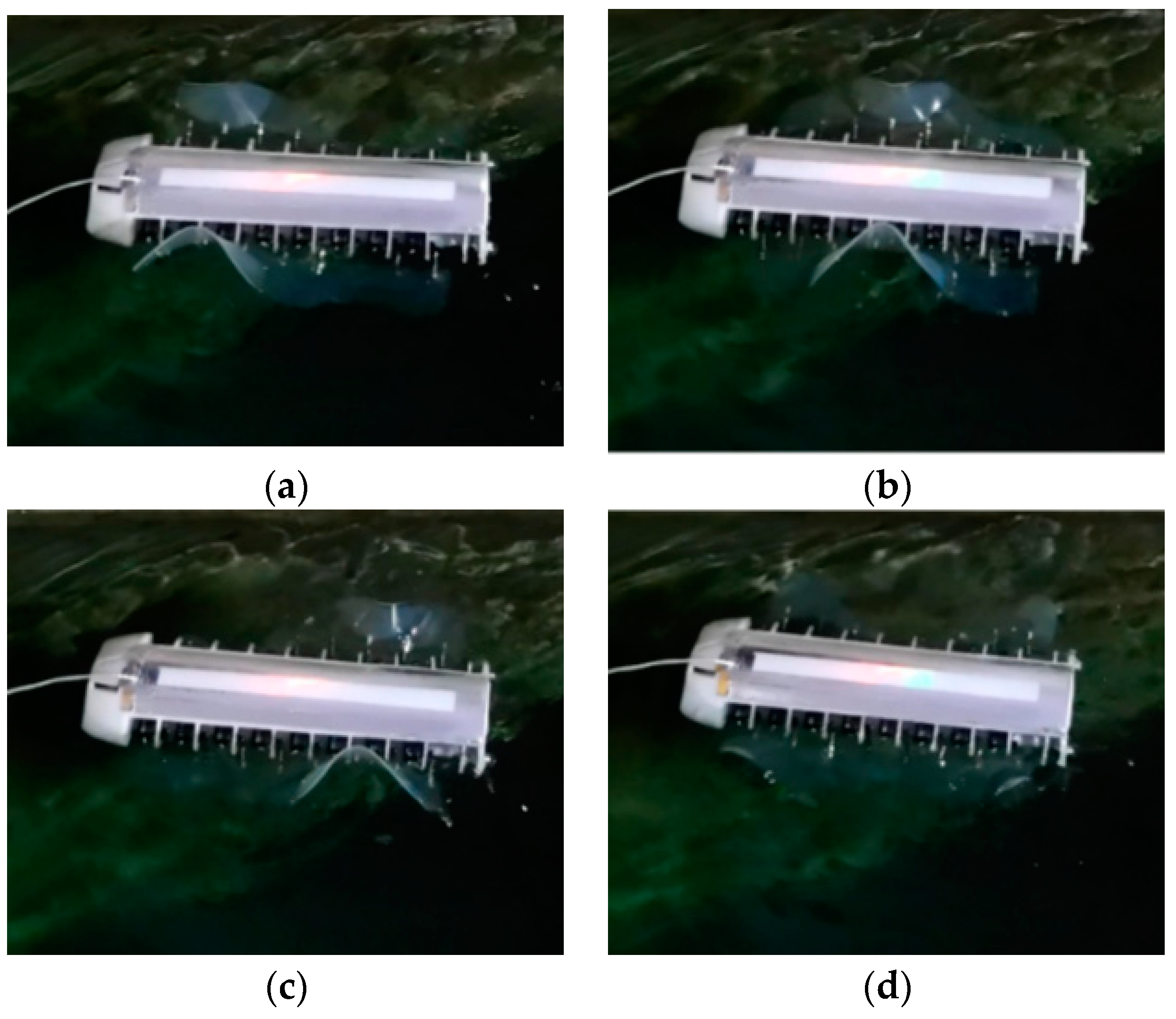
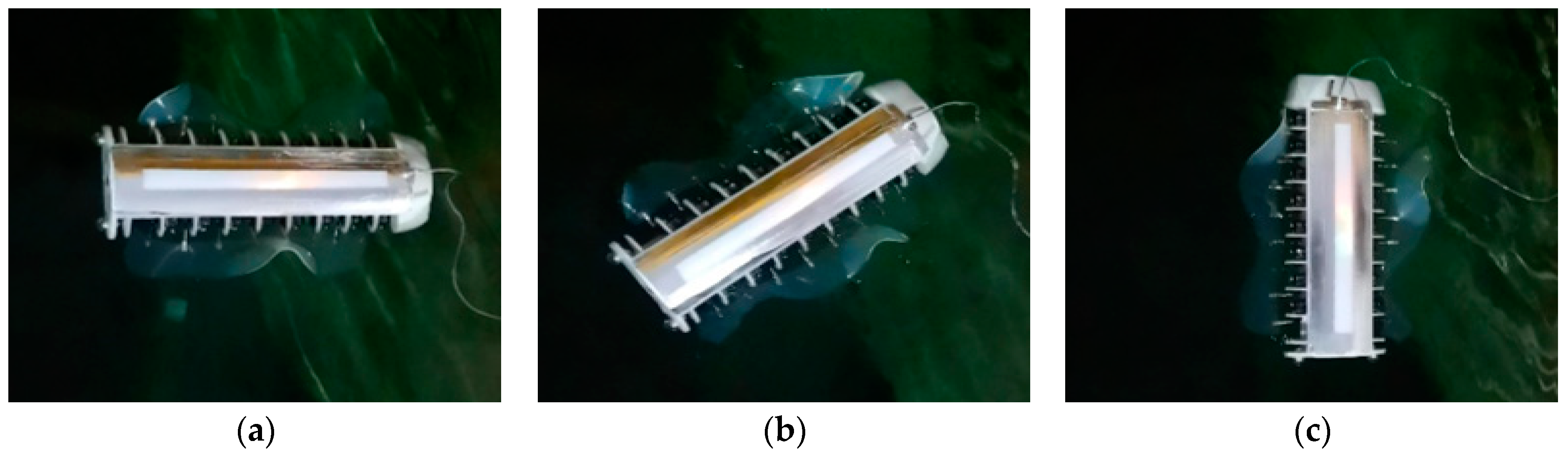
Currently, most research on the propulsion performance of banded fins derives from biomimetic sources rather than focusing directly on the banded fins themselves, as demonstrated in this paper. There is a limited number of studies that investigate the hydrodynamic performance and optimization of fin types for practical banded fins used in underwater vehicles. In this study, we focus on the biomimetic analysis of the long dorsal fin of banded fish, establishing a wave description equation for the fin and using numerical simulation methods to investigate its wave propulsion mechanism. Additionally, we perform a comprehensive analysis of hydrodynamic performance by varying key parameters, thereby establishing the relationship between the wave thrust coefficient of the banded fin and these parameters. We also investigate the hydrodynamic performance of the fin surface by varying the angle of attack and implementing chamfering on the front and rear edges to optimize the overall hydrodynamic efficiency of the banded fins. Based on these numerical results, we design a bio-inspired vehicle equipped with a banded fin propulsion system and conduct underwater tests to validate the rationale behind its design. This study contributes to bio-inspired propulsion systems by establishing a kinematic and hydrodynamic model for the banded fin based on the MPF mode. Through numerical simulations, the hydrodynamic performance of the fin is analyzed under typical conditions, revealing how key parameters like wave number, swing amplitude, and wave frequency affect oscillatory thrust. This study also explores the impact of angle of attack and edge chamfering on optimizing hydrodynamic efficiency. This study differs from existing research by focusing directly on the hydrodynamic performance and optimization of banded fins for underwater propulsion, rather than relying on general biomimetic models. It develops a specific kinematic and hydrodynamic model, analyzes key parameters like wave number and swing amplitude, and investigates the effects of angle of attack and edge chamfering on propulsion efficiency.

2. Simulations Based on the Analysis of Banded Fin Fluctuations

2.1. Wave Model

Firstly, the kinematic modeling of the banded fin’s undulatory motion is depicted in Figure 1. A dynamic model describing the oscillatory motion of the elongated dorsal fin is established based on its structural characteristics. Since the thin dorsal fin of the hairtail has a negligible influence on its movement pattern, it can be neglected. The primary motion patterns of the dorsal fin in banded fish are analyzed, and variations in wave amplitude and fin surface height are disregarded to propose the following assumptions regarding the oscillation of the banded fin: (1) The propulsion generated by the banded fin is considered to exhibit pure rigid motion; (2) The banded fin is assumed to possess negligible thickness, with uniform wave amplitude and height; (3) The surface of the banded fin is treated as a smooth curved surface, for which we derive a wave equation in polar coordinates (Equation (1)).

$$\left\{\begin{array}{l}x=u\hfill \\ y=\rho \cdot \cos \left[{\theta }_{\max }\cdot \sin \left(2\pi \cdot {\displaystyle \frac{u}{\lambda }}+\omega \cdot t+{\phi }_0\right)\right]\hfill \\ z=\rho \cdot \sin \left[{\theta }_{\max }\cdot \sin \left(2\pi \cdot {\displaystyle \frac{u}{\lambda }}+\omega \cdot t+{\phi }_0\right)\right]\hfill \end{array}\right.$$

(1)

where $u$ represents the parameter $x$, ${\theta }_{\max }$ denotes the maximum swing angle, $\lambda$ signifies the wavelength of the banded fin fluctuation, $\omega$ represents the angular frequency, $t$ denotes time, and ${\phi }_0$ indicates the initial phase. The boundary conditions for the surface motion of the fin body are as follows: the length of the banded fin, $L$, is 0.9 m, corresponding to $x$ in Equation (1). The height of the fin surface ranges $\rho$ from 0.05 m to 0.2 m. The time $t=0$, and the initial phase ${\phi }_0=0$.

Figure 1. Kinematic modeling of the banded fin, where u represents the wave speed and v denotes the velocity of the banded fin.

2.2. Method

2.2.1. Numerical Simulation Method

In the oscillation process of the banded fin, the Reynolds number is defined by the fluid velocity, characteristic length, and dynamic viscosity. The minimum fluid velocity in the study is 0.18 m/s, with the characteristic length defined as the fin length, which is 0.9 m. The calculated Reynolds number exceeds 4000, indicating the presence of turbulent characteristics in the flow field. To simulate and calculate turbulence, the Reynolds time average (RANS) method is employed while ensuring mass conservation through continuity and momentum conservation equations for incompressible fluids:

$${\displaystyle \frac{\mathsf{\partial }{\mathrm{u}}_{\mathrm{i}}}{\mathsf{\partial }{\mathrm{x}}_{\mathrm{i}}}}=0$$

(2)

$$\rho {\displaystyle \frac{d{u}_i}{dt}}=-{\displaystyle \frac{\mathsf{\partial }p}{\mathsf{\partial }{x}_i}}+{\displaystyle \frac{\mathsf{\partial }}{\mathsf{\partial }{x}_i}}\left[\mu \left({\displaystyle \frac{\mathsf{\partial }{u}_i}{\mathsf{\partial }{x}_j}}+{\displaystyle \frac{\mathsf{\partial }{u}_j}{\mathsf{\partial }{x}_j}}-{\displaystyle \frac{2}{3}}{\delta }_{ij}{\displaystyle \frac{\mathsf{\partial }{u}_1}{\mathsf{\partial }{x}_1}}\right)\right]+{\displaystyle \frac{\mathsf{\partial }}{\mathsf{\partial }{x}_j}}\left(-\rho \overline{u_i^{\prime }{u}_j^{\prime }}\right)$$

(3)

where $\rho$ represents the fluid density, $u_{i,j}$ denotes the velocity in the $x_{i,j}$ direction, $\mu$ represents the dynamic viscosity, $t$ represents time, $p$ represents pressure, $\overline{u_i^{\prime }}$ represents the fluctuating velocity in the $x_i$-direction, and $-\rho \overline{u_i^{\prime }{u}_j^{\prime }}$ represents the Reynolds stress term.

The realizable $k-\epsilon$ model is employed for computation, while the transport equation governing turbulent kinetic energy and its dissipation rate is expressed as follows:

$$\rho {\displaystyle \frac{\mathsf{\partial }k}{\mathsf{\partial }t}}={\displaystyle \frac{\mathsf{\partial }}{\mathsf{\partial }{x}_i}}\left[\left(\mu +{\displaystyle \frac{{\mu }_t}{{\sigma }_k}}\right){\displaystyle \frac{\mathsf{\partial }k}{\mathsf{\partial }{x}_i}}\right]+G_k+G_b-\rho \epsilon -Y_m$$

(4)

$$\rho {\displaystyle \frac{\mathsf{\partial }\epsilon }{\mathsf{\partial }t}}={\displaystyle \frac{\mathsf{\partial }}{\mathsf{\partial }{x}_i}}\left[\left(\mu +{\displaystyle \frac{{\mu }_t}{{\sigma }_{\epsilon }}}\right){\displaystyle \frac{\mathsf{\partial }\epsilon }{\mathsf{\partial }{x}_i}}\right]+\rho C_1{S}_{\epsilon }-\rho C_2{\displaystyle \frac{{\epsilon }^2}{k+\sqrt{v\epsilon }}}+C_{1\epsilon }{\displaystyle \frac{\epsilon }{k}}{C}_{3\epsilon }{G}_b$$

(5)

$C_1=max[0.43,\eta /\eta +5]$, $\eta =Sk/\epsilon$, where $C_2$ and $C_{1\epsilon }$ are constants; ${\sigma }_k$ and ${\sigma }_{\omega }$ are the turbulent Prandtl numbers for $k$ and $\omega$, $G_k$ represents the production of turbulent kinetic energy due to the mean velocity gradient, $G_b$ represents the production of turbulent kinetic energy due to buoyancy effects, and $Y_m$ represents the effect of compressible turbulent fluctuations on the total dissipation rate.

In this study, we employ thrust coefficient ($C_T$) and propulsion efficiency ($\eta$) to characterize the propulsion performance under different fin surface fluctuation states. By comparing $C_T$ and $\eta$ values for banded fins, we demonstrate the advantages and disadvantages of their propulsion performance in various operating conditions. The thrust coefficient is defined as the ratio between actual total thrust and ideal total thrust (the latter being obtained from a one-dimensional isentropic fully expanding flow). The equation can be expressed as follows:

$$C_T={\displaystyle \frac{T}{\rho \cdot f^2\cdot A^2\cdot L^2}}$$

(6)

where $T$ represents the thrust, $\rho$ denotes the fluid density, $f$ represents frequency, $L$ represents fin length, and $A$ signifies the fluctuation amplitude of the banded fin; the undulatory propulsion efficiency of the banded fin is defined as the ratio between its actual propulsion power and the total input power, as depicted in the subsequent equation:

$$\eta ={\displaystyle \frac{{\overline{T}}_x\cdot V_{inlet}}{{\overline{P}}_{hydro}}}$$

(7)

where $V_{inlet}$ represents the incoming flow velocity, ${\overline{T}}_x$ denotes the average thrust generated in the $x-axis$ direction (i.e., along the incoming flow velocity), and ${\overline{P}}_{hydro}$ signifies the average input power over a given period, as shown in the following equation:

$$P_{hydro}={\displaystyle {\sum }_{k=0}^n{\displaystyle {\sum }_{i=0,j_1\in {\complement }_{U}i,j_2\in {\complement }_U{j}_1}^2\left({\sigma }_i+{\tau }_{j_{i}i}+{\tau }_{j_{2}i}\right)\cdot \overrightarrow{i}\cdot {\overrightarrow{v}}_i\cdot {\overrightarrow{S}}_k}}$$

(8)

where ${\sigma }_i$ represents the normal stress along the $I$$axis$, ${\tau }_{ij}$ denotes the shear stress in the $j$ direction within a plane perpendicular to the $I$$axis$, and $\overrightarrow{i}$ signifies the unit vector for the $I$$axis$. Additionally, ${\overrightarrow{S}}_k$ refers to a mesh face element, $k$ corresponds to its assigned mesh face number, n indicates the total count of mesh faces, and finally, ${\overrightarrow{v}}_i$ represents the velocity vector aligned with the centroid position $i$ of said mesh face element.

2.2.2. Dynamic Mesh Method

Owing to the periodic undulatory motion of the banded fin, this study utilizes a dynamic mesh approach to update the mesh at the moving boundary. For flux $\varphi$, (the flux refers to the velocity flux, and in the case of moving grids, it denotes the correction of the velocity flux due to grid deformation), within any control volume $V$, the conservation equation can be expressed as follows:

$${\displaystyle \frac{d}{dt}}{\displaystyle {\int }_V\rho }\varphi dV+{\displaystyle {\int }_{\mathsf{\partial }V}\rho \varphi \left(\stackrel{\rightharpoonup }{u}-\stackrel{\rightharpoonup }{u_s}\right)\cdot d\stackrel{\rightharpoonup }{A}}={\displaystyle {\int }_{\mathsf{\partial }V}\mathrm{\Gamma }\nabla \varphi \cdot d\stackrel{\rightharpoonup }{A}}+{\displaystyle {\int }_V{S}_{\varphi }dV}$$

(9)

where $\rho$ represents the fluid density, $\stackrel{\rightharpoonup }{u}$ denotes the velocity vector of the fluid, $\stackrel{\rightharpoonup }{u_s}$ represents the deformation velocity of the grid, $\mathrm{\Gamma }$ represents the diffusion coefficient, $S_{\varphi }$ represents the source term of flux $\varphi$, and $\mathsf{\partial }V$ represents the boundary of the control volume.

The first term in the aforementioned equation can be expressed using a first-order backward difference, yielding

$${\displaystyle \frac{d}{dt}}{\displaystyle {\int }_V\rho }\varphi dV={\displaystyle \frac{{\left(\rho \varphi V\right)}^{n+1}-{\left(\rho \varphi V\right)}^n}{\Delta \mathrm{t}}}$$

(10)

where $n$ and $n+1$ represent the values at the $n$ and $n+1$ time steps; the volume $V^{n+1}$ at the $n+1$ step is calculated using Equation (11):

$$V^{n+1}=V^n+{\displaystyle \frac{dV}{dt}}\Delta t$$

(11)

where $dV/dt$ represents the volume derivative of the control body. To satisfy the grid conservation law, the volume derivative of the control body is calculated using Equation (12):

$${\displaystyle \frac{dV}{dt}}={\displaystyle {\int }_{\mathsf{\partial }V}\stackrel{\rightharpoonup }{u_g}\cdot d\stackrel{\rightharpoonup }{A}}={\displaystyle \sum _j^{n_f}\stackrel{\rightharpoonup }{u_{g,j}}\cdot \stackrel{\rightharpoonup }{A_j}}$$

(12)

where $n_f$ represents the number of control surfaces and $\stackrel{\rightharpoonup }{A_j}$ represents the area vector of surface $j$. The scalar product for each control surface, denoted as $\stackrel{\rightharpoonup }{u_{g,j}}\cdot \stackrel{\rightharpoonup }{A_j}$, is determined according to Equation (13):

$$\stackrel{\rightharpoonup }{u_{g,j}}\cdot \stackrel{\rightharpoonup }{A_j}={\displaystyle \frac{\delta V_j}{\Delta t}}$$

(13)

At time step $\Delta t$, $\delta V_j$ represents the volume swept by the control surface of control volume $j$.

2.2.3. Grid Partitioning and Grid Independent Verification

Based on these considerations, an incompressible fluid model is selected and the effects of gravity are incorporated into the transient solution. The moving grid method is employed for updating, while the SIMPLE (Semi-Implicit Method for Pressure-Linked Equations) algorithm is utilized for convergence. Discretization is performed using a second-order upwind scheme, and a no-slip condition is imposed at the wall boundary. After verifying convergence, a time step of 0.005 s is set, and the UDF (User-Defined Function) program defines the wave form of the banded fin to control the movement of each grid node according to the aforementioned wave equation.

The banded fin model is developed under the constraints of fixed supports by defining the ratio of wavelength to fin length, the swing angle, and the fluctuation frequency. The wavelength-to-fin length ratio used is 1, the oscillation angle is 30°, and the oscillation frequency is 1 Hz. Since the fin surface position is fixed, the fluid domain size and position are fixed when drawing the fluid domain, ensuring symmetry. After performing the chamfering operation, the fluid domain is sufficiently large compared to the fin due to the refined mesh region, which ensures that the simulation results are reliable. The computational domain division is illustrated in Figure 2.

Figure 2. Computational domain and boundary conditions.

The scale of the fluid domain is determined by the length of the banded fin; the large domain measures 3 L × 0.8 L × 0.8 L, while the small domain measures 1.4 L × 0.4 L × 0.4 L; and the interface between these two domains serves as the data transfer surface. The negative direction of the right x-axis is designated as the velocity inlet, positioned at a distance of one fin length from the tip of the banded fin. Similarly, on the left x-axis, the pressure outlet is located in the positive direction, also at a distance of one fin length from its endpoint. The upper, lower, left and right boundary surfaces are defined as symmetry planes. The meshing process is updated during each time step, making it challenging to accurately capture boundary layer thicknesses consistently throughout all steps taken; hence, an encryption technique is applied within smaller domains while larger domains expand, starting from interface mesh size shared with smaller ones, and separate divisions are made for fin surface meshing. The volume mesh uses tetrahedral elements, while the surface mesh consists of triangular elements; the resulting mesh division outcomes are illustrated in Figure 3.

Figure 3. Mesh division. (a) Mesh division of all domains. (b) Mesh division of small domain. (c) Mesh division of fin surface.

Based on the model established in Figure 2, the grid is divided into seven groups with varying numbers of volume grids: 1.01 million, 2.51 million, 2.92 million, 3.48 million, 3.84 million, 4.59 million and 6.79 million, respectively, generated for numerical simulation under the conditions described in Section 2.2. The thrust coefficients under each operating condition are then calculated and presented in Table 1.

Table 1. Independence validation of volume grid.

Series	Number of Volume Grids (Million)	CT	Relative Error (%)
1	1.01	0.3065	-
2	2.51	0.3486	12.08
3	2.92	0.3571	2.38
4	3.48	0.3636	1.79
5	3.84	0.3643	0.193
6	4.59	0.3650	0.192
7	6.79	0.3657	0.192

Mesh independence is verified by applying a mesh size gradient and selecting the optimal mesh configuration through a relative error analysis. Seven mesh sets were considered, as the relative error progressively decreases from the first to the fifth set, with no significant change in the relative error between the sixth and seventh sets. The results indicate that for a grid count greater than or equal to 3.84 million, the numerical calculation exhibits a low relative error, with an error rate of less than 0.2% compared to the previous set of volume grids. Therefore, in order to strike a balance between computational accuracy and efficiency, we have opted for a volume grid count of 3.84 million for our calculations.

Furthermore, the accuracy of the proposed numerical method for calculating efficiency in this study is also influenced by the number of grids employed. Hence, it is imperative to ascertain the grid independence of the fin surface. The corresponding calculation results are presented in Table 2.

Table 2. Independence validation of fin surface grid.

Series	Number of Surface Grids (Thousand)	Input Power (W)	Relative Error (%)
1	202.5	2.7950	-
2	677.5	2.8605	2.29
3	985.0	2.8795	0.66
4	1432.5	2.8832	0.13

The results in Table 2 demonstrate that for a number of fin surface grids greater than or equal to 985,000, the relative error compared to the previous group is below 0.7%, indicating that the grid size has minimal impact on the numerical simulation. Considering both calculation accuracy and efficiency, we have selected a surface grid size of 985,000 for our calculations.

3. Periodic Hydrodynamic Performance Analysis of Variable Parameters for a Banded Fin

The control variable method was used to perform a hydrodynamic numerical analysis on the key parameters of the banded fin, effectively clarifying its periodic motion characteristics. In order to better demonstrate the general motion law of banded fins under variable wave parameters, the intermediate conditions of incoming flow velocity, wavelength-to-fin length ratio, wave frequency, and swing angle are taken as typical conditions, with wavelength-to-fin length ratio $\lambda /L=1$, swing angle ${\theta }_{\max }={30}^{\circ }$, fluctuation frequency $f=1\mathrm{Hz}$, and incoming flow velocity $v=0.36 \mathrm{m}/\mathrm{s}$. The variable parameters are listed in Table 3, and will not be repeated here. According to the computational results, the thrust, lateral force, lift, and input power converge within 10 cycles. Therefore, the averaged values of these quantities are determined over multiple cycles between 11 and 14. These values are then normalized using dimensionless numbers for further analysis. The variables for the parameter analysis conditions in this study are closely related to the dimensions and parameters of the actual prototype. These conditions are also based on the variable control method employed by Zeng et al. [33] in his investigation of the hydrodynamic performance of flexible fins, where the simulation results were found to be satisfactory.

Table 3. Variable parameter analysis conditions.

Parameter	$\mathit{\lambda }/\mathit{L}$	$\mathit{v}$ (m/s)	${\mathit{\theta }}_{\max }$ (°)	$\mathit{f}$ (Hz)
	0.4, 0.6, 0.8, 1, 1.5, 2	0.36	30	1
	1	0.18, 0.36, 0.54, 0.72, 0.81, 0.9	30	1
	1	0.36	5, 15, 30, 45, 60	1
	1	0.36	30	0.5, 1, 2, 4

3.1. Effect of Wave Parameters on the Hydrodynamic Performance of the Banded Fins

3.1.1. Variable Wavelength to Fin Length

The time–domain curve of the thrust coefficient over a single period for the banded fin is shown in Figure 4a. It reveals two distinct peaks and troughs in the thrust coefficient curve under different wave numbers within one period, indicating that the thrust coefficient undergoes two fluctuations per cycle. When the wavelength-to-fin length ratio is either relatively large ($\lambda /L\ge 2$) or relatively small ($\lambda /L\le 0.4$), secondary fluctuations are diminished but maintain the same pattern. The amplitude of each peak and trough varies, especially at $\lambda /L=1.5$, where the larger trough has an amplitude approximately three times greater than the smaller one, while the larger peak is about 1.1 times greater than the smaller peak. When $\lambda /L\le 0.8$, as the wavelength-to-fin length ratio increases, the overall thrust coefficient values increase over the full period.

Figure 4. Hydrodynamic characteristic curve: (a) thrust coefficient variation curve at different wavelength–fin length ratios; (b) the change curve of force coefficient at different wavelength–fin length ratios; (c) hydrodynamic characteristic curves of fin length ratios at different wavelengths.

The change curves of the average thrust, lateral force, and lift coefficients at varying wavelength-to-fin length ratios are illustrated in Figure 4b. It is evident that when $\lambda /L\le 1$, the coefficients for average thrust, lateral force, and lift exhibit a significant increase with an increasing $\lambda /L$ ratio. In contrast, when $\lambda /L>1$, the thrust coefficient shows a more gradual increase, while the growth rates of the lateral force and lift coefficients slightly decelerate. Overall, across the variable wave number parameters, the coefficients for lateral force and lift consistently exceed those for thrust, with this trend becoming more pronounced as the wavelength-to-fin length ratio increases. Furthermore, the wave–fin ratio appears to have a minimal impact on the occurrence of the lift coefficient, surpassing the thrust coefficient.

The curve illustrating the thrust coefficient and hydrodynamic efficiency at a constant flow velocity of 0.36 m/s is shown in Figure 4c. It reveals that the optimal efficiency point occurs at approximately $\lambda /L=0.6$, where the thrust coefficient reaches 0.06. At this point, the power and drag generated by the banded fin are balanced, resulting in a propulsion efficiency of around 57.6%. For $\lambda /L\le 0.6$, the thrust coefficient becomes negative, and the negative available work is not reflected in the efficiency curve. As $\lambda /L$ increases, propulsion efficiency initially declines rapidly, then experiences a slight rise, followed by a continuous decrease, showing two extreme values and two peaks.

An analysis of the reasons for this phenomenon is further provided in Table 4. According to Equation (7), the propulsion efficiency $\eta$ is directly proportional to both the thrust coefficient $C_T$ and the incoming flow velocity $V$, while being inversely proportional to the input power magnitude ${\overline{P}}_{hydro}$. When considering a given incoming flow velocity $V$, the propulsion efficiency $\eta$ solely depends on the ratio of thrust coefficient to input power. The growth rate ratio between these two parameters R1/R2 reflects the growth rate of efficiency, which will not be discussed in Section 3.1.2, Section 3.1.3 and Section 3.1.4. It can be observed that both thrust coefficient and input power increase with an increase in wave–fin ratio. Generally, as the wavelength–fin length ratio increases, there is a gradual decrease followed by a relatively stable trend in propulsion efficiency.

Table 4. Growth rate of thrust coefficient and input power at different wavelength–fin length ratios.

$\lambda /L$	$C_T$	Growth Rate R1	${\overline{P}}_{hydro}$ (W)	Growth Rate R2	R1/R2	Emerging Tendency
0.4	−0.0076	-	0.00397	-	-	-
0.6	0.06019	894.52%	0.291710	7240.50%	-	-
0.8	0.14524	141.30%	1.381411	373.56%	0.3783	$\downarrow$
1	0.20953	44.27%	2.879549	108.45%	0.4082	$\downarrow$
1.5	0.29054	38.66%	3.324975	15.47%	2.4990	$\uparrow$
2	0.30399	4.63%	7.576854	127.88%	0.0362	$\downarrow$

3.1.2. Variable Swing Amplitude

The surface of the banded fin is segmented into multiple straight lines along the $yz$-plane. At any position $-x=xi$, the straight lines on the surface rotate around the fixed $x-axis$. The wave motion of the fin surface can thus be conceptualized as a combination of numerous straight lines rotating about the $x-axis$. Under specified conditions, where the fin surface height defines the radius of the polar axis $\rho$, different swing angles ${\theta }_{\max }$ correspond to varying magnitudes of the vibration amplitude A for the banded fin. Through numerical simulations, we obtained a time–domain curve representing the variation in the thrust coefficient with swing angle within a single period (Figure 5). The thrust coefficient exhibits a distinct “W” shape across different swing angles ${\theta }_{\max }$ oscillating twice per cycle with alternating peaks and troughs. The pattern of time-averaged thrust remains consistent, featuring large peak, large trough, small peak, and small trough in sequence, with only their amplitudes varying. At ${\theta }_{\max }=5^{\circ }$, the values of both the large peak and large trough are nearly identical. Overall, the thrust coefficient increases as the swing angle amplitude ${\theta }_{\max }$ increases.

Figure 5. Hydrodynamic characteristic curve: (a) change curve of thrust coefficient at different swing angles; (b) the change curve of force coefficient under different swing angles; (c) hydrodynamic characteristic curves under different swing angles.

The variation curves for average thrust, lateral force, and lift coefficients under different swing amplitude angles are illustrated in Figure 5b. The analysis shows that for ${\theta }_{\max }\le {20}^{\circ }$, the average thrust coefficient increases significantly with the rise in $\lambda /L$. However, for ${\theta }_{\max }>{20}^{\circ }$, the resistance caused by the rapid swinging of the fin surface increases considerably, resulting in a more gradual increase in the thrust coefficient. This effect can be explained by the increase in angular velocity of each individual fin line as the swing angle grows, while maintaining a constant fluctuation frequency. Once the angular velocity exceeds a certain threshold, frictional resistance escalates, weakening the contribution to forward propulsion and leading to a more moderate increase in the total thrust coefficient. When ${\theta }_{\max }$ is around 20°, the lateral force coefficient becomes smaller than the thrust coefficient, and at ${\theta }_{\max }\approx {50}^{\circ }$, even the lift coefficient starts to decrease relative to the thrust coefficient. In general, the lift coefficients tend to exceed the thrust coefficients across most swing angles.

The thrust coefficient and hydrodynamic efficiency curve are shown in Figure 5c. It is clear that the optimal efficiency point occurs at a swing angle ${\theta }_{\max }$ of 45°, yielding a propulsion efficiency of approximately 37.9%. For swing angles ${\theta }_{\max }\le {30}^{\circ }$, the propulsion efficiency of the banded fins remains relatively constant. However, between 30° and 45°, the propulsion efficiency increases rapidly as the swing angle increases. Beyond ${\theta }_{\max }>{45}^{\circ }$, further increases in the swing angle lead to a decline in propulsion efficiency. These trends are summarized based on the calculated input power values, as presented in Table 5. Notably, both thrust Tx and input power ${\overline{P}}_{hydro}$ increase proportionally with increasing swing angle ${\theta }_{\max }$. At ${\theta }_{\max }={45}^{\circ }$, the growth rate of input power ${\overline{P}}_{hydro}$ is significantly smaller than that of thrust Tx, resulting in a substantial amplification of propulsion efficiency under this condition compared to other scenarios where the growth rate of propulsion efficiency $\eta$ is relatively slower.

Table 5. Growth rate of thrust and input power at different swing angles.

${\theta }_{max}$ (°)	$T_x$ (N)	Growth Rate R1	${\overline{P}}_{hydro}$ (W)	Growth Rate R2	R1/R2	Emerging Tendency
5	−0.00519	-	0.02893	-	-	-
15	0.32578	−6373.63%	0.5754	1888.98%	-	-
30	1.694205	420.03%	2.8795	400.42%	1.048937	$\uparrow$
45	3.837232	126.49%	3.6483	26.70%	4.737671	$\uparrow$
60	6.19157	61.36%	6.7289	84.44%	0.726618	$\downarrow$

3.1.3. Variable Oscillation Frequency

The time–domain curve of the thrust coefficient variation with fluctuation frequency f in a single period of the banded fin is presented in Figure 6a. It can be observed that the change pattern of the thrust coefficient at different frequencies is consistent with other operating conditions, i.e., it oscillates twice per cycle. Generally speaking, as the fluctuation frequency increases, the thrust coefficient gradually rises.

Figure 6. Hydrodynamic characteristic curve: (a) change curve of thrust coefficient in one week under different fluctuation frequencies; (b) force coefficient curves at different frequencies; (c) hydrodynamic characteristic curves at different frequencies.

The change curves of average thrust, lateral force, and lift coefficients at different fluctuation frequencies are shown in Figure 6b. It is clear that the coefficients of thrust, lateral force, and lift gradually increase as the fluctuation frequency ($f$) rises. For frequencies of $f$ ≤ 1.5 Hz, the force coefficients in all three directions exhibit a rapid growth rate with increasing frequency. However, for $f$ > 1.5 Hz, this growth rate tends to level off. This behavior is explained by the fact that under a constant swing angle ${\theta }_{\max }$, higher fluctuation frequencies lead to larger angular velocities of the individual fin elements. When the swing angular velocity exceeds a certain threshold, frictional resistance from the rapid fin oscillation significantly increases, resulting in greater total resistance, which diminishes the forward propulsion force. As a result, the total thrust coefficient exhibits a more gradual increase. Generally, the thrust coefficient remains consistently higher than the lateral force coefficient but lower than the lift coefficient.

The curve of the thrust coefficient and hydrodynamic efficiency under an inflow velocity of $v$ = 0.36 m/s is depicted in Figure 6c. It can be observed that the optimal efficiency point occurs at a fluctuation frequency $f$ of 1 Hz, with a propulsion efficiency of 37.9% at this juncture.

The propulsion efficiency of the banded fin remains almost constant when $f\le 1$ Hz, but gradually decreases with increasing fluctuation frequency ($f>1$ Hz) at a decreasing rate. This trend is reflected in Table 6, which shows that as f increases, so does the input power ${\overline{P}}_{hydro}$, albeit at varying rates. Specifically, the growth rate of propulsion efficiency $\eta$ gradually increases until it peaks at $f=2$ Hz and then slows down.

Table 6. Growth rate of thrust and input power at different frequencies.

$f (Hz)$	$T_x$ (N)	Growth Rate R1	${\overline{\mathbf{P}}}_{hydro}$ (W)	Growth Rate R2	R1/R2	Emerging Tendency
0.25	−0.14423	-	−0.022473	-	-	-
0.5	0.02477	117.17%	0.032151	243.06%	-	-
1	1.6942	6739.02%	2.879549	8856.10%	0.7609	$\downarrow$
2	13.3533	688.17%	26.71582	827.78%	0.8314	$\downarrow$
4	69.8112	422.80%	227.2708	750.70%	0.5632	$\downarrow$

3.1.4. Variable Flow Rate

Considering a wavelength-to-fin length ratio of $\lambda /L=1$, a maximum swing amplitude angle ${\theta }_{\max }={30}^{\circ }$, and a fluctuation frequency $f$ of 1 Hz, the magnitude of the advance coefficient $J$ is solely dependent on the inflow velocity $v$, as indicated by the following equation:

$$J={\displaystyle \frac{v}{f\cdot \lambda }}$$

(14)

The time–domain curve illustrating the variation in the thrust coefficient with the advance velocity coefficient in a single period of the banded fin is calculated and presented in Figure 7a, where it can be observed that, for a given wavelength-to-fin length ratio ($\lambda /L$) of 1, the trend of thrust coefficient under different advance rate coefficients ($J$) follows a similar pattern to other operational conditions, wherein the thrust coefficient undergoes two fluctuations within each cycle and exhibits consistent amplitudes at both peaks and troughs. Generally, an increase in the advance rate coefficient ($J$) leads to a decrease in the thrust coefficient; moreover, when $J$ equals 1.0, the thrust coefficient becomes negative.

Figure 7. Hydrodynamic characteristic curve: (a) change curve of thrust coefficient in one week under different advance coefficients; (b) change curve of force coefficient at different advance speeds; (c) undulating fin open water characteristic curve.

The change curves of the average thrust, lateral force, and lift coefficients under varying advance rate coefficients $J$ are shown in Figure 7b. It is evident that as $J$ increases, the thrust, lateral force, and lift coefficients gradually decrease, contributing to a smoother reduction in speed. When other oscillation parameters remain constant, an increase in the advance velocity coefficient $J$ results in a higher incoming flow velocity $v$ while maintaining the same flow area. This increased flow velocity causes a rise in form drag, leading to a significant increase in total resistance and, consequently, a reduction in forward propulsion force. As the flow velocity continues to rise, the growth rate of form drag slows down, resulting in a more gradual decrease in the total thrust coefficient. Overall, the thrust coefficient remains consistently higher than the lateral force coefficient, but it is smaller than the lift coefficient.

The open water characteristic curve of the banded fin is presented in Figure 7c, revealing that the optimum efficiency point occurs at a propulsion rate coefficient $J=0.6$, with a corresponding propulsion efficiency of 45.8%. For $J\le 0.6$, the propulsion efficiency gradually increases as the propulsion rate coefficient rises; however, for $J>0.6$, an increase in the propulsion rate coefficient leads to a decrease in propulsion efficiency (as shown in Table 7).

Table 7. Growth rate of thrust and input power at different advance speed coefficients.

$J$	$T_x·v$ (W)	Growth Rate R1	${\overline{P}}_{hydro}$ (W)	Growth Rate R2	R1/R2	Emerging Tendency
0	0.0000	-	5.71987	-	-	-
0.2	0.5907	-	3.30760	−42.17%	-	-
0.4	0.6099	3.26%	2.87954	−12.94%	−0.2517	$\uparrow$
0.6	0.3952	−35.20%	0.859330	−70.16%	0.5017	$\uparrow$
0.8	0.0989	−74.98%	0.304581	−64.56%	1.1615	$\downarrow$
1	−0.1994	−301.64%	0.004558	−98.50%	-	-

The increase in the advance rate coefficient is observed to result in a decrease in input power, with the rate of decrease gradually accelerating. Similarly, as the advance rate factor $J$ increases, there is a reduction in hydrodynamic input power ${\overline{P}}_{hydro}$. For $J<0.6$, the propulsion efficiency growth rate shows a gradual increase until reaching its peak at $J=0.6$, after which it gradually slows down. It should be noted that when $J=1.0$, negative thrust occurs and thus this particular operating condition is not included in this analysis.

3.2. Analysis of Propulsion Mechanism of Banded Fin Swimming

This section analyzes the causes of macroscopic force in the above section from the perspectives of pressure field, velocity field and vorticity field. The classical condition mentioned in Section 3 is adopted as the validation case in this section, i.e., wavelength-to-fin length ratio $\lambda /L=1$, swing angle ${\theta }_{\max }={30}^{\circ }$, fluctuation frequency $f=1$ Hz, and advance coefficient $J=0.4$.

3.2.1. Analysis of the Pressure Field

The pressure field cloud map of the fin surface at different time points within a single period is depicted under typical working conditions, as illustrated in Figure 8:

Figure 8. Cloud image of pressure field on the surface of banded fin: (a) t/T = 0; (b) t/T = 0.25; (c) t/T = 0.5; (d) t/T = 0.75.

When t/T = 0 (Figure 8a), the leading edge of the oscillating fin experiences significant suction forces, with the negative pressure region forming a band at the location of maximum suction. When t/T = 0.75 (Figure 8d), the pressure region on the fin surface moves rearward as the wave propagates. In the localized pressure areas between the wave crest and trough, the fin exhibits backward oscillatory motion, which is characterized by a backward inclination that generates thrust. The pressure distribution forms a sinusoidal curve on the fin surface, intersecting the zx-plane, with the first stationary point located after the first wave crest. At this moment, both the pressure and suction amplitudes are high, with the maximum suction pressure reaching 350 Pa and the pressure amplitude at 101 Pa. The area of the pressurized region exceeds half of the fin’s wetted surface area, with the main pressure area (shown in red in the contour map) and suction side (shown in deep blue in the contour map) being larger than in other moments. According to the thrust coefficient curve over a single cycle, the generated thrust at this moment is the highest compared to the other three time points.

When t/T = 0.25 (Figure 8b), the suction and pressure are alternately distributed at the leading edge of the oscillating fin, with the maximum suction occurring at the wave crest. Compared to the previous moment, the pressure region on the fin moves rearward as the wave propagates. In the localized pressure areas between the wave crest and trough, the fin exhibits backward oscillatory motion, characterized by a backward inclination that generates thrust. The pressure distribution forms a sinusoidal curve on the fin surface, intersecting the zx-plane, with the first stationary point located after the first wave crest. At this time, both the pressure and suction amplitudes are smaller, with the maximum suction pressure around 156 Pa and the pressure amplitude around 51 Pa. The area of the pressurized region is less than half of the fin’s wetted surface area, and the main pressure area (shown in red in the contour map) and suction side (shown in deep blue in the contour map) are significantly reduced compared to t/T = 0 (Figure 8a). According to the thrust coefficient curve, the generated thrust at this time is the second smallest among the four time points.

When t/T = 0.5 (Figure 8c), a small localized pressure region forms on the outer side of the leading edge of the oscillating fin, corresponding to the pressure amplitude. The leading surface exhibits negative pressure, with suction acting significantly at the wave crest. The maximum suction pressure reaches 345 Pa, and the pressure amplitude is 96 Pa. According to the thrust coefficient curve, the generated thrust at this time is the second largest among the four time points.

When t/T = 0.75 (Figure 8d), the pressurized region on the oscillating fin moves rearward with its oscillatory motion, reaching the first wave crest after the leading edge. Due to the upward motion of the front half of the oscillating fin, the water flow slides along the fin surface and reaches a localized pressure region, as shown in the figure. The oscillating fin then pushes the water upward at an oblique angle, generating thrust and lift. At this time, the rear portion of the wave crest experiences localized suction, corresponding to the suction amplitude. The pressure distribution forms a sinusoidal curve on the fin surface, intersecting the zx-plane, with the first stationary point located after the first wave crest. The maximum suction pressure reaches 147 Pa, and the pressure amplitude is 50 Pa. At this moment, the pressure amplitude decreases, and the area of the pressurized region exceeds half of the fin’s wetted surface area, with the main pressure area located toward the front of the fin. According to the thrust coefficient curve, the generated thrust at this time is the smallest among the four time points.

3.2.2. Analysis of the Passing Velocity Field

Velocity field cloud images on the fin surface at different time points ($y$ = 0.1 m) were captured during a typical single cycle, as illustrated in Figure 9.

Figure 9. Cloud image of velocity field on the surface of banded fin: (a) t/T = 0; (b) t/T = 0.25; (c) t/T = 0.5; (d) t/T = 0.75.

Figure 9 demonstrates that at t/T = 0, the flow velocity reaches a maximum of 0.75 m/s, while at t/T = 0.25 and t/T = 0.75, it decreases. Flow acceleration predominantly occurs at the trailing edge of the fin, supporting the “scoop-and-push” propulsion mechanism. Incomplete acceleration and shorter strokes at t/T = 0.25 and t/T = 0.75 result in lower thrust, whereas full acceleration and longer strokes at t/T = 0 and t/T = 0.5 generate greater thrust. Therefore, the propulsion of the undulating fin is driven by its oscillatory motion, with variations in stroke length leading to periodic fluctuations in thrust.

3.2.3. Analysis of the Passing Vorticity Field

The Q-criterion, set to a value of 0.01, is applied to generate the vorticity cloud map of the velocity field, as illustrated in Figure 10.

Figure 10. Vorticity field cloud map of the banded fin. (a) Tail view (b) 45 degree oblique overhead view (c) Side view.

Figure 10 demonstrates that the oscillatory motion of the banded fin generates two types of vortices: a streamwise vortex from the fin’s maximum height and a ring vortex at the fin’s crest. These vortices intertwine, leading to significant fluid acceleration at their intersection, indicating possible jet flow.

Different oscillation modes result in variations in power input to the fin, impacting propulsion efficiency. Fish improve efficiency primarily through inertial forces, leading-edge suction, and vortex energy utilization. Inertial force is the main contributor to thrust and overall efficiency, while leading-edge suction optimizes the fin’s shape for a low-pressure region. Fish can effectively harness vortices through counter-stroking motion, creating reverse Kármán vortex streets that extract energy from the water. This utilization of vortex energy significantly enhances propulsion efficiency, particularly when reverse vortices are induced through undulatory motion, generating additional jet flow forces.

4. Hydrodynamic Performance Optimization of Banded Fins

According to the mechanism analysis, the thrust force generated by the banded fin is primarily the reaction force exerted by the fin surface on the fluid. In this paper, we explore how varying the angle of attack affects the interaction between the oblique plate and the water pushed by the fin surface, and we discuss its relationship with the resulting propulsion force. Furthermore, building on the understanding of the banded fin’s propulsion mechanism, we examine variations in pressure distribution and investigate how alterations in fin shape influence hydrodynamic performance. Lastly, an optimization method for improving the hydrodynamic performance of the banded fin is proposed. This approach aims to enhance thrust efficiency by fine-tuning key parameters, such as fin shape, angle of attack, and movement patterns, to achieve optimal propulsion in various flow conditions.

4.1. Hydrodynamic Performance of Banded Fins Under Varying Attack Angles

According to the definition of the airfoil on the angle of attack (Triantafyllou, 1996), the front and back edges of the banded fin are connected with straight lines, which are characterized as the chord of the ribbon fin. The angle between the chord and the direction of the incoming flow velocity is denoted as the angle of attack, as illustrated in Figure 11.

Figure 11. Angle of attack of the banded fin.

As the governing equation for banded fin motion is based on an angle of attack of zero, transformation from a satellite coordinate system to earth coordinate system should be performed during the calculation of the variable angle of attack. The transformation matrix for the coordinate system is as follows:

$$\left[\begin{array}{c}{X}^{\prime }\\ Y^{\prime }\\ Z^{\prime }\end{array}\right]=\left[\begin{array}{ccc}\cos \beta & 0& -\sin \beta \\ 0& 1& 0\\ \sin \beta & 0& \cos \beta \end{array}\right]\left[\begin{array}{l}X\hfill \\ Y\hfill \\ Z\hfill \end{array}\right]$$

(15)

The banded fin with variable angle of attack is controlled by the transformed equation. To ensure control over other variables in the calculation process, the hydrodynamic parameters of the banded fin with variable angle of attack are determined under the typical condition, whose wavelength-to-fin length ratio $\lambda /L=1$, swing angle ${\theta }_{\max }={30}^{\circ }$. fluctuation frequency $f=1$ Hz, and incoming flow velocity $v=0.36 \mathrm{m}/\mathrm{s}$. Once the calculated forces and input power have achieved periodic convergence, the effective result is obtained by averaging their single-period quantities over multiple convergence periods, as presented in Table 8.

Table 8. Effect of variable angle of attack on hydrodynamic performance of banded fin.

$\mathbf{\beta }$ (°)	$C_{Tx}$	Growth Rate (%)	$\mathbf{\eta }$ (%)	Growth Rate (%)	$C_{Ty}$	Growth Rate (%)	$C_{Tz}$	Growth Rate (%)
−15	0.2126	1.47	0.258	21.97	0.2257	14.71	0.0200	−93.76
−10	0.1433	−31.61	0.188	−11.11	0.1795	−8.77	0.5160	60.77
−5	0.1878	−10.33	0.355	67.72	0.1897	−3.57	0.4272	33.11
0	0.2095	-	0.211	-	0.1968	-	0.3209	-
5	0.2243	7.05	0.439	107.57	0.2128	8.17	0.2023	−36.96
10	0.2202	5.09	0.356	68.08	0.2158	9.67	0.0748	−76.67
15	0.0745	−64.42	0.077	−63.64	0.1817	−7.66	0.6544	103.90

The hydrodynamic performance of the banded fin is significantly influenced by variations in the angle of attack $\beta$. In conjunction with the parameters provided in the table, it can be observed that when $\beta$ is set to −15°, 5°, and 10°, there is a slight increase in thrust coefficient, a significant improvement in propulsion efficiency, and a notable decrease in lift coefficient. Notably, at an angle of attack of 5°, both thrust coefficient and rate of change for propulsion efficiency reach their maximum values while minimizing the reduction in lift coefficient.

When the angle of attack $\beta$ is −10°, −5°, and 15°, a significant decrease in the thrust coefficient is observed. The change in propulsion efficiency exhibits considerable variation, with the propulsion efficiency at a −5° angle of attack showing the highest increase of 67.72%. At an angle of attack of −10° and 15°, there is a respective decrease in propulsion efficiency by 11.11% and 63.64%, while the lift coefficient experiences a notable increase. This trend contrasts with that observed at an angle of attack of −15° and 10°, indicating that the inclined plate’s water-pushing force can be decomposed into two components: thrust and lift.

The following section will further analyze the impact of varying attack angles on the hydrodynamic performance of the undulating fin from the perspective of macroscopic force fluctuations, as illustrated in Figure 12.

Figure 12. The variation curve of the internal force coefficient over a single cycle at different angles of attack: (a) x-axis thrust coefficient; (b) y-axis thrust coefficient; (c) z-axis thrust coefficient.

The analysis shows that varying the angle of attack produces a consistent “W” shape in the thrust coefficient curve. Angles of −10°, −5°, and 15° result in lower thrust than 0°, with irregular peak and trough patterns. At −15° and 10°, thrust alternates with 0°, while 5° produces higher thrust for most of the cycle. Peaks at −15°, 5°, and 10° match those at 0°, but troughs are larger, increasing the thrust coefficient. Lateral force peaks and troughs decrease at −10°, −5°, and 15°, but increase at −15°, 5°, and 10°. Lift is highly affected by the angle of attack, while thrust sees smaller increases and larger decreases, with minimal impact on lateral force.

Figure 13 illustrates that changes in the angle of attack have a minimal effect on the lateral force coefficient, a moderate effect on the thrust coefficient, and a pronounced impact on the lift coefficient. Propulsion efficiency reaches its maximum, 46%, near an angle of 5°. With the exception of −10° and 15°, most other angles of attack contribute positively to propulsion efficiency.

Figure 13. (a) Variation in force coefficients at different angles of attack; (b) open water performance curves at different angles of attack.

According to Equation (7), propulsion efficiency $\eta$ is directly proportional to the thrust coefficient $C_{Tx}$ and incoming flow velocity $V$, and inversely proportional to input power ${\overline{P}}_{hydro}$. Under constant flow velocity, propulsion efficiency depends on the ratio of the thrust coefficient to input power, and their relative growth rates reflect the efficiency increase. Table 9 shows that input power decreases at all angles compared to 0°. At −10° and 15°, the thrust coefficient decreases faster than input power, leading to reduced efficiency, while at other angles, the smaller drop in thrust coefficient results in improved efficiency.

Table 9. Thrust coefficient and input power growth rate at variable angle of attack.

$\mathbf{\beta }$ (°)	$C_{Tx}$	Growth Rate R1	${\overline{P}}_{hydro}$ (W)	Growth Rate R2	R1/R2	Emerging Tendency
−15	0.2126	1.47%	2.3955	−16.81%	−0.0875	$\uparrow$
−10	0.1433	−31.61%	2.2154	−23.06%	1.3705	$\downarrow$
−5	0.1878	−10.33%	1.5395	−46.54%	0.2219	$\uparrow$
0	0.2095	-	2.8795	-	-	$-$
5	0.2243	7.05%	1.4850	−48.43%	−0.1455	$\uparrow$
10	0.2202	5.09%	1.8003	−37.48%	−0.1357	$\uparrow$
15	0.0745	−64.42%	2.8178	−2.14%	30.045	$\downarrow$

In summary, changes in attack angle mainly affect propulsion efficiency by altering input power, with a notable improvement at a 5° angle. The attack angle significantly impacts the lift coefficient, with less effect on the thrust and lateral force coefficients.

4.2. Analysis of the Impact of Varying Oncoming Attack Angles on Hydrodynamic Forces

In this section, pressure contour plots, velocity field diagrams, and velocity streamlines are utilized to analyze the impact of variable attack angles. A cross-sectional analysis at y = 0.1 m along the wave fin surface, with an attack angle of 5°, is compared to the zero attack angle condition.

4.2.1. Comparison of Pressure Contour Plots

The pressure contour plots for the oncoming flow at an attack angle of 5° and at an attack angle of zero are shown in Figure 14.

Figure 14. Velocity field nephograms of the fin at different time steps with and without attack angle. (a) Attack angle of 5° t/T = 0; (b) angle of attack 0° t/T = 0; (c) attack angle of 5° t/T = 0.2; (d) attack angle of 0° t/T = 0.2; (e) attack angle of 5° t/T = 0.4; (f) attack angle of 0° t/T = 0.4; (g) attack angle of 5° t/T = 0.6; (h) attack angle of 0° t/T = 0.6; (i) attack angle of 5° t/T = 0.8; (j) attack angle of 0° t/T = 0.8.

It is evident that the pressure cloud images at different times exhibit some differences between the two conditions. Overall, the pressure distribution at a 5° angle of attack is more uniform, with a larger area on the pressurized side. During the “catching water” phase, both the pressure and suction magnitudes are relatively low, while they increase significantly during the “pushing water” phase, which aligns with the observed variations in the thrust coefficient curve over the cycle.

4.2.2. Comparison of Velocity Contour Plots

The head-on velocity field cloud images for both the 5° angle of attack and the 0° angle of attack are presented in Figure 15.

Figure 15. Velocity field nephogram of the fin at different time intervals with and without an angle of attack. (a) Attack angle of 5° t/T = 0; (b) angle of attack 0° t/T = 0; (c) attack angle of 5° t/T = 0.2; (d) attack angle of 0° t/T = 0.2; (e) attack angle of 5° t/T = 0.4; (f) attack angle of 0° t/T = 0.4; (g) attack angle of 5° t/T = 0.6; (h) attack angle of 0° t/T = 0.6; (i) attack angle of 5° t/T = 0.8; (j) attack angle of 0° t/T = 0.8.

The velocity field generated by the fin section at $y$ = 1/9 L (0.1m), under angle of attack conditions of 5° and 0°, is depicted in Figure 15. It can be observed that in the zero angle of attack condition (the left side of Figure 15), the primary water propulsion occurs solely at the tail section of the fin surface. However, at a 5° angle of attack, all segments—tail, front, and middle—actively contribute to water propulsion, resulting in significantly expanded work exerted on the water flow and increased effective mass involved compared to the zero angle of attack condition, consequently leading to substantial enhancement in propulsion efficiency.

4.2.3. Comparison of Velocity Streamline Fields

The velocity flow line field diagram for a 5° and 0° attack angle is shown in Figure 16, which represents the end section of the banded fin.

Figure 16. Comparison of velocity and streamline fields at the fin’s end section with and without an angle of attack. (a) Attack angle of 5° t/T = 0; (b) angle of attack 0° t/T = 0; (c) attack angle of 5° t/T = 0.2; (d) attack angle of 0° t/T = 0.2; (e) attack angle of 5° t/T = 0.4; (f) attack angle of 0° t/T = 0.4; (g) attack angle of 5° t/T = 0.6; (h) attack angle of 0° t/T = 0.6; (i) attack angle of 5° t/T = 0.8; (j) attack angle of 0° t/T = 0.8.

The water flow at the end of the banded fin exhibits high velocity and experiences significant variations in the flow field. To analyze the influence of vortices on hydrodynamic performance, we intercepted and plotted the velocity streamline field diagram of the fin surface’s end section (Figure 16). Within this flow field, two large vortices are generated with opposite normal directions. Notably, a distinct water acceleration phenomenon is observed in the middle of these vortices, which further supports our conjecture regarding potential jet generation at this location. At an angle of attack of 5° (right side of Figure 16), vortex streamlines become denser and exhibit larger vorticity, effectively harnessing vortex energy and contributing significantly to enhanced propulsion efficiency.

4.3. Influence of Fillet on the Hydrodynamic Performance of the Banded Fin

The pressure field cloud diagram of the banded fin reveals a distinct negative pressure field at its leading edge. In this section, we analyze the impact of altering the fin surface shape on the hydrodynamic performance of the banded fin by introducing chamfers to both its front and back edges.

Similarly, a typical condition whose wavelength-to-fin length ratio $\lambda /L=1$ and swing angle ${\theta }_{\max }={30}^{\circ }$ was employed, with the leading edge, trailing edge, and front and rear edges being rounded individually. The chamfering radius R was set to 1/6 L (0.15 m). The resulting fin surface model after chamfering is illustrated in Figure 17:

Figure 17. The shape of the fin surface after chamfering.

The calculation is conducted under the typical operational conditions of wavelength-to-fin length ratio $\lambda /L=1$, swing angle ${\theta }_{\max }={30}^{\circ }$, fluctuation frequency $f=1$ Hz, and incoming flow velocity $v=0.36 \mathrm{m}/\mathrm{s}$, with the corresponding results presented in Table 10.

Table 10. Effect of different fin surface shapes on hydrodynamic performance of banded fin.

Chamfer Position	$C_{Tx}$	Growth Rate (%)	$\mathbf{\eta }$ (%)	Growth Rate (%)	$C_{Ty}$	Growth Rate (%)	$C_{Tz}$	Growth Rate (%)
/	0.2095	-	21.18	-	0.1968	-	0.3209	-
Front edge	0.1970	−5.97	49.85	135.38	0.1845	−6.22	0.3033	−5.50
Rear edge	0.1990	−5.01	38.28	80.72	0.1869	−5.01	0.2993	−6.73
Front and rear edge	0.1846	−11.86	36.87	74.05	0.1742	−11.48	0.2882	−10.19

The hydrodynamic performance of the banded fin can be significantly influenced by altering its fin surface shape. By reducing the wetted surface area, the water push area in a single cycle is decreased, resulting in varying degrees of force reduction in three directions. Simultaneously, optimizing the shape of the negative pressure zone at the leading edge of the banded fin can substantially enhance its propulsion efficiency. The chamfering efficiency at the leading edge is approximately 135% higher than that without chamfering, while at the trailing edge it is around 80%, and about 74% for further improvement.

The impact of variable attack angle on the hydrodynamic performance of the banded fin will be analyzed from the perspective of macroscopic force fluctuations, as illustrated in Figure 18.

Figure 18. Variation curve of internal force coefficient in one period under different chamfer shapes: (a) x-axis thrust coefficient; (b) y-axis thrust coefficient; (c) z-axis thrust coefficient.

Altering the fin surface shape affects the hydrodynamic performance of the banded fin, reducing thrust, lateral force, and lift coefficients compared to the no-fillet case. While the general “W” shape of the force curves remains, peaks and troughs shift, with notable decreases in trough values for both thrust and lateral force, and significant changes in the lift coefficient. Forward and aft fillet cases show similar patterns, but differ from the non-fillet condition. These changes likely result from modifications to the flow field caused by the fin shape alteration.

4.4. Analysis of the Impact of Fillet Shape on Hydrodynamic Performance

In this section, the influence of chamfering on the hydrodynamics of banded fins is analyzed by using the single-period instantaneous pressure cloud diagram with different fin surface shapes and the cross-sectional velocity flow line field comparison diagram at the end of the fin surface.

4.4.1. Comparison of Pressure Contour Plots on Chamfered Fin Surface

This is analyzed from the angle of pressure cloud map. The instantaneous pressure cloud image under the three chamfer conditions of t/t = 0~t/t = 0.8 is shown in Figure 19.

Figure 19. Comparison of velocity and streamline fields at the fin’s end section with and without an chamfering. (a) Leading edge rounding t/T = 0; (b) trailing edge rounding t/T = 0; (c) leading and trailing edge rounding t/T = 0; (d) leading edge rounding t/T = 0.2; (e) trailing edge rounding t/T = 0.2; (f) leading and trailing edge rounding t/T = 0.2; (g) leading edge rounding t/T = 0.4; (h) trailing edge rounding t/T = 0.4; (i) leading and trailing edge rounding t/T = 0.4; (j) leading edge rounding t/T = 0.6; (k) trailing edge rounding t/T = 0.6; (l) leading and trailing edge rounding t/T = 0.6; (m) leading edge rounding t/T = 0.8; (n) trailing edge rounding t/T = 0.8; (o) leading and trailing edge rounding t/T = 0.8.

It can be observed that the shape and distribution of the pressure area on the fin surface are significantly altered by chamfering. In comparison to the no-chamfering condition, the negative pressure zone at the leading edge no longer exhibits a perpendicular strip to the flow velocity but instead follows a streamlined pattern along the curvature of the chamfered angle at the fin surface’s edge in alignment with flow direction. This configuration optimizes viscous pressure resistance caused by banded fin fluctuations. By comparing and analyzing pressure distribution cloud maps for front and back chamfering conditions, it is discovered that both reduce the range of fin surface coverage, resulting in lower propulsion efficiency compared to only front chamfering conditions. Simultaneously, wet surface area reduction after chamfering diminishes water displacement volume and subsequently reduces thrust force.

4.4.2. Comparison of Velocity Streamline Fields on Chamfered Fin Cross-Section

The velocity field distribution of the fin surface’s end section under chamfering and non-chamfering conditions is illustrated in Figure 20.

Figure 20. Comparison of velocity streamlines of fin terminal section with and without filleting. (a) Apply rounding t/T = 0; (b) without rounding t/T = 0; (c) apply rounding t/T = 0.2; (d) without rounding t/T = 0.2; (e) apply rounding t/T = 0.4; (f) without rounding t/T = 0.4; (g) apply rounding t/T = 0.6; (h) without rounding t/T = 0.6; (i) apply rounding t/T = 0.8; (j) without rounding t/T = 0.8.

It can be observed that, compared to the non-chamfering condition (left side of Figure 20), the streamline distribution at the end section of the chamfered fin surface is denser and exhibits greater vorticality. Consequently, it exerts a more pronounced acceleration effect on water flow, leading to a wider distribution of peak velocities. Similar to varying the angle of attack, optimizing the shape of the fin surface also induces changes in the flow field. Moreover, chamfering enhances vortex energy utilization, thereby reducing input power requirements and improving wave propulsion efficiency for banded fins.

5. Design and Research of a Bio-Inspired Aquatic Vehicle Equipped with Banded Fins

5.1. Design of the Bionic Prototype for the Banded Fin

The banded fin bionic thruster consists of two parts: the main boat body and bionic banded fins on both sides, with the size, waveform, and motion parameters of the fins determined by numerical calculations. To meet the vehicle’s operational requirements, several considerations were taken into account: (1) a low-resistance shape design was necessary to reduce energy consumption caused by liquid resistance during long-term underwater operation; (2) multiple banded fins were required to ensure cruising stability and maneuverability; and (3) spatial planning was crucial for accommodating various sensors while maintaining overall hydrodynamic characteristics unaffected by steering gear presence.

The overall flat shape of the vehicle helps with its low drag underwater. The primary mechanical structure of the vehicle employs a steering mechanism-connecting rod-bio-inspired banded fin connection mode. The steering gear is fixed on the thickness structure reserved within the main body of the bio-inspired propeller. The connecting rod mechanism directly links with the steering gear, and the adjustable fixed position connects with the bio-inspired banded fin. Toda Y, et al. [34] used numerical simulations to replicate the physical model of banded fins, conducting experiments to reveal the underlying motion mechanisms of the fins. The waveform of the bionic vehicle’s banded fins follows the pattern described in Equation (1), enabling a more comprehensive comparison and validation between the numerical simulations and prototype experiments. The bio-inspired banded fin utilizes silicone rubber with a hardness rating of 60 degrees, ensuring its exceptional elasticity meets all required properties for a banded fin. The oscillatory propulsion system of the bio-inspired propulsor consists of nine high-precision servos on each side, offering excellent control over the oscillation. This setup allows the servos to precisely replicate the natural motion of banded fins, enhancing hydrodynamic performance while improving response speed and stability. The nine-servo configuration enables the propulsor to accommodate various bio-inspired fin shapes, with users simply needing to replace the fin to switch between different oscillatory patterns for diverse operational conditions. Additionally, the system offers high adjustability, enabling the control of oscillation frequency and amplitude to meet the propulsion requirements of different aquatic environments.

The underwater bio-inspired thruster is equipped with an embedded propeller in its tail, enhancing its risk-avoidance capability. This design generates increased thrust and higher propulsion efficiency compared to an external propeller. Moreover, it reduces the noise generated by the propeller to some extent, thereby improving the vehicle’s stealth performance. Subsequently, the main body of the vehicle, steering gear, damping linkage mechanism, and bio-inspired banded fin are assembled to achieve an overall effect, as depicted in Figure 21:

Figure 21. Overall effect of the vehicle.

The control strategy employed in this prototype involves utilizing a single-chip microcomputer to govern the multi-channel PWM for achieving synchronized motion of multiple servo motors, encompassing swing, frequency, and other motion parameters. Through RS-485 bus control, instructions are transmitted to the address bits of each serial port to facilitate the desired movement of the servo motors. The specific control process is outlined as follows: (1) A 24-channel servo motor controller (ZL-IS2) is utilized by the computer to edit control signals. To enable offline remote control and remote operation, a Bluetooth control module is integrated into the 24-channel servo motor control board, allowing action manipulation under offline conditions. (2) Power supply and data transmission are essential for steering gear control and necessitate integration into a wire group. The power-data line set connects the 24-channel servo motor control board with the respective steering gears. The serial number on the PWM interface of the 24-channel servo motor control board corresponds to that of each controlled steering gear. A flowchart demonstrating the control sequence of the prototype is presented in Figure 22:

Figure 22. A flowchart demonstrating the control sequence of the prototype.

Connect the installed signal cable of the steering gear to the designated position on the 24-steering-gear control board, ensuring proper arrangement. Utilize computer software for 24-way steering gear control to input varying pulse numbers and time steps, while setting the input wavelength–fin ratio to 1, swing angle to 30°, and frequency $f$ = 1 Hz. The resulting control effect is illustrated in Figure 23.

Figure 23. Physical display of waveform at different times. (a) t/T = 0; (b) t/T = 0.25; (c) t/T = 0.5; (d) t/T = 0.75.

5.2. Experimental Assessment of Aquatic Environments

In order to validate the hydrodynamic rationality of the banded fin bio-inspired propeller’s shape design, assess whether the motion mechanism’s strength meets water propulsion requirements, and evaluate the feasibility of the control system design, we conducted actual water testing on the vehicle to obtain empirical data regarding the banded fin’s propulsion performance in aquatic environments in this section.

The direct movement exercise test was initially conducted, which is shown in Figure 24. Synchronized motion of the bio-inspired banded fins on both sides of the main body of the bio-inspired fin thrusters is required for direct propulsion, ensuring that the thrust generated by both fins acts in unison to counteract resistance from the main body.

Figure 24. The direct movement exercise test. (a) t/T = 0; (b) t/T = 0.25; (c) t/T = 0.5; (d) t/T = 0.75.

Subsequently, the turning test was conducted, encompassing two distinct modes of turning movement: 1. zero-turn radius mode where the vehicle remains stationary at its center position and 2. turning around an obstacle with a specific radius. These two turning conditions necessitate contrasting banded fin control methods.

For the zero-turn radius mode, the bio-inspired banded fins on both sides of the banded fin bio-inspired thruster are controlled to move in an identical waveform and frequency but in opposite directions; for the mode with turning radius, which can be achieved by regulating the asymmetry of bio-inspired banded fins on both sides, the thrust generated by the bio-inspired banded fins on the inner side of the turn is minimized, while on the outer side it is maximized. In cases where the turning radius is small, it becomes possible to immobilize the inner side of the turn while allowing normal movement on the outer side. The spot turning process is illustrated in Figure 25, among the various conditions.

Figure 25. The spot turning test in counterclockwise direction. (a) The start of the spot turning test (b) The mid-phase of the spot turning test (c) The end of the spot turning test.

6. Conclusions

The hydrodynamic performance of the banded fin is investigated using a computational fluid dynamics method, and a numerical model is established to ensure the independence of mesh parameters. Additionally, experimental verification is conducted to validate the accuracy of the numerical model, ensuring reliable results for the numerical simulation. The contributions made in this study can be summarized as follows:

By simulating various working conditions, including variations in fin length ratio, swing amplitude, fluctuation frequency, and flow velocity, we conducted a comprehensive analysis of the periodic changes in hydrodynamic coefficients and propulsion efficiency exhibited by the banded fin. Additionally, we fitted thrust coefficient curves under different working conditions. In a single period, the force coefficient exhibits a “W” fluctuation curve, wherein the thrust coefficient surpasses the lateral force coefficient but remains lower than the lift coefficient. When the wave–fin ratio is 0.6, the maximum hydrodynamic efficiency can reach 57.6%. For a banded fin with a wave–fin ratio of 1, optimal propulsion performance is achieved at a swing angle of 45°, frequency of 1 Hz, and propulsion factor of 0.6. Simultaneously, through an analysis of the pressure field distribution, velocity field, and flow velocity diagrams, we deduced the undulation propelling mechanism of the banded fin, where water is moved obliquely toward the rear during fin oscillation, providing valuable insights into the thrust generation process.

Based on the propulsion mechanism of the banded fin, an analysis was conducted to assess its hydrodynamic performance by varying the angle of attack and the shape of the fin surface. Notably, adjusting the angle of attack to 5° significantly improved propulsion efficiency. Additionally, chamfering both the anterior and posterior edges of the fin surface further enhanced efficiency compared to non-chamfered conditions. These findings underscore that optimizing the shape of the negative pressure region at the leading edge can effectively boost the hydrodynamic performance of the banded fin.

Finally, based on the numerical calculations of the hydrodynamic performance of the band fin, we have designed a prototype of an underwater bio-inspired propeller with the bio-inspired banded fin as its primary propulsion mode. Subsequently, real water movement tests were conducted to successfully demonstrate forward and backward movements, in-place turning, and radius turning motions, all meeting the design requirements.

References

- Breder, C.M. The locomotion of fishes. J. Zool. 1926, 4, 159–297. [Google Scholar] [CrossRef]
- Webb, P.W. Maneuverability—General issues. J. IEEE J. Ocean. Eng. 2004, 29, 547–555. [Google Scholar] [CrossRef]
- Lighthill, M.J. Note on the swimming of slender fish. J. Fluid Mech. 1960, 9, 305–317. [Google Scholar] [CrossRef]
- Lighthill, M.J. Aquatic animal propulsion of high hydromechanical efficiency. J. Fluid Mech. 1970, 44, 265–301. [Google Scholar] [CrossRef]
- Lighthill, M.J. Large-Amplitude Elongated-Body Theory of Fish Locomotion. J. Proc. R. Soc. Lond. 1971, 179, 125–138. [Google Scholar] [CrossRef]
- Cheng, J.Y.; Zhuang, L.X.; Tong, B.G. Analysis of swimming three-dimensional waving plate. J. Fluid Mech. 1991, 232, 341–355. (In Chinese). Available online: https://kns.cnki.net/kcms2/article/abstract?v=lxIxReJOxlcEVv4UWwh8rlEEjDcGwTL-75qc_Bi8NVIAdcW92neuPKVv1eqHywa52bFDflcL8trIueLGYpPPUTjOTW4wmTdvuJpQJIZbtrG54m7ak6LDGO0m8bW9K36e&uniplatform=NZKPT&language=CHS (accessed on 1 October 2024). [CrossRef]
- Tong, B.G.; Zhuang, L.X.; Cheng, J.Y. Hydrodynamics of fish propelled by wavy oscillation. J. Mech. Eng. 1991, 3, 17–26. (In Chinese). Available online: https://kns.cnki.net/kcms2/article/abstract?v=lxIxReJOxlesniFKcqjo4sL6gM6WwwnUXkzsNFtDHLoJpvYhjl6HmRu9p3YClH8_fdbiRZneQhbeojh1v2nBIzt2hD5-tAAJTSSFvaKoE34atNTML0sa0Id1ZevBbQvd&uniplatform=NZKPT&language=CHS (accessed on 5 October 2024).
- Cheng, J.Y.; Blickhan, R. Bending moment distribution along swimming fish. J. Theor. Biol. 1994, 168, 337–348. (In Chinese) [Google Scholar] [CrossRef]
- Mchenry, M.J.; Pell, C.A.; Long, J.H. Mechanical Control of Swimming Speed: Stiffness and Axial Wave Form in Undulating Fish Models. J. Exp. Biol. 1995, 198, 2293–2305. [Google Scholar] [CrossRef]
- Pedley, T.J.; Hill, S.J. Large-Amplitude Undulatory Fish Swimming: Fluid Mechanics Coupled to Internal Mechanics. J. Exp. Biol. 1999, 202, 3431–3438. [Google Scholar] [CrossRef] [PubMed]
- Miriam, A.A. Mechanical Properties of the Dorsal Fin Muscle of Seahorse (Hippocampus) and Pipefish (Syngnathus). J. Exp. Zool. 2002, 293, 561–577. [Google Scholar] [CrossRef]
- Long, J.H.; Adcock, J.B.; Root, R.G. Force Transmission Via Axial Tendons in Undulating Fish: A Dynamic Analysis. J. Comp. Biochem. Physiol. 2002, 133A, 911–929. [Google Scholar] [CrossRef] [PubMed]
- Zhang, Y.H.; Jia, L.B.; Zhang, S.W.; Yang, J.; Low, K.H. Computational research on modular undulating fin for biorobotic underwater propulsor. J. Bionic Eng. 2007, 4, 25–32. [Google Scholar] [CrossRef]
- Zhang, D.B.; Hu, D.W.; Shen, L.C.; Xie, H.B. Design of an artificial bionic neural network to control fish-robot’s locomotion. J. Neurocomput. 2008, 71, 648–654. [Google Scholar] [CrossRef]
- Liu, F.F.; Lee, K.M.; Yang, C.J. Hydrodynamics of an Undulating Fin for a Wave-Like Locomotion System Design. J. IEEE/ASME Trans. Mechatron. 2012, 17, 554–562. [Google Scholar] [CrossRef]
- Zhang, D.; Huang, Q.G.; Pan, G.; Yang, L.M.; Huang, W.X. Vortex dynamics and hydrodynamic performance enhancement mechanism in batoid fish oscillatory swimming. J. Fluid Mech. 2022, 930, 1–32. [Google Scholar] [CrossRef]
- Zhou, H.; Hu, T.J.; Xie, H.B.; Zhang, D.B.; Shen, L.C. Computational and experimental study on dynamic behavior of underwater robots propelled by bionic undulating fins. J. Sci. China Technol. Sci. 2010, 53, 2966–2971. [Google Scholar] [CrossRef]
- Zeng, X.F.; Xia, M.H.; Luo, Z.R.; Shang, J.Z.; Xu, Y.Z.; Yin, Q. Design and Control of an Underwater Robot Based on Hybrid Propulsion of Quadrotor and Bionic Undulating Fin. J. Mar. Sci. Eng. 2022, 10, 1327. [Google Scholar] [CrossRef]
- He, J.; Cao, Y.; Huang, Q.; Cao, Y.; Tu, C.; Pan, G. A new type of bionic manta ray robot. In Proceedings of the Global Oceans 2020: Singapore—U.S. Gulf Coast, Biloxi, MS, USA, 5–30 October 2020; pp. 1–6. [Google Scholar] [CrossRef]
- Xing, C.; Cao, Y.; Cao, Y.H.; Pan, G.; Huang, Q.G. Asymmetrical Oscillating Morphology Hydrodynamic Performance of a Novel Bionic Pectoral Fin. J. Mar. Sci. Eng. 2022, 10, 289. [Google Scholar] [CrossRef]
- Wei, C.; Hu, Q.; Li, S.; Zhang, T.; Shi, X. Hydrodynamic performance analysis of undulating fin propulsion. Phys. Fluids 2023, 35, 091906. [Google Scholar] [CrossRef]
- Shi, F.; Xin, J.; Jin, Q.; Yang, Y.; Wan, L. Hydrodynamics investigation of a three-dimensional fish swimming in oblique flows by a ghost cell method. Phys. Fluids 2024, 36, 111902. [Google Scholar] [CrossRef]
- Chen, L.; Hu, Q.; Zhang, H.; Tong, B.; Shi, X.; Jiang, C.; Sun, L. Research on underwater motion modeling and closed-loop control of bionic undulating fin robot. Ocean Eng. 2024, 299, 117400. [Google Scholar] [CrossRef]
- Li, G.; Ma, P.; Fang, X.; Li, G.; Liu, G.; Cheng, H. Study on thrust increase characteristics of separated undulating fins. Ocean Eng. 2024, 313, 119292. [Google Scholar] [CrossRef]
- Li, G.; Liu, G.; Ma, P.; Li, G.; Fang, X. Study on stable thrust of separated undulating fins. Ocean Eng. 2024, 306, 118046. [Google Scholar] [CrossRef]
- Shi, X.; Hu, Q.; Zhang, T.; Li, S.; Zeng, Y. Research on hydrodynamic performance of 2D undulating fin in the wake of a semi-cylinder. Ocean Eng. 2024, 308, 118055. [Google Scholar] [CrossRef]
- Sun, G.; Wang, Z.; Ling, H.; Dou, P.; Yan, Y. Investigation on the propulsive efficiency of undulating fin propulsor. Ocean Eng. 2024, 312, 119113. [Google Scholar] [CrossRef]
- Vu, Q.T.; Duong, V.T.; Nguyen, H.H.; Nguyen, T.T. Optimization of swimming mode for elongated undulating fin using multi-agent deep deterministic policy gradient. Eng. Sci. Technol. Int. J. 2024, 56, 101783. [Google Scholar]
- Wei, C.; Li, S.; Hu, Q. Hydrodynamic performance analysis of formations of dual three-dimensional undulating fins. Ocean Eng. 2024, 305, 117939. [Google Scholar] [CrossRef]
- Xia, D.; Lei, M.; Li, Z.; Shi, Y. A combined IB-LB method for predicting the hydrodynamics of bionic undulating fin thrusters. Ocean Eng. 2024, 303, 117790. [Google Scholar] [CrossRef]
- Yu, D.; Che, T.; Zhang, H.; Li, Y.; Sun, D.; Wang, Z. Terrestrial locomotion stability of undulating fin amphibious robots: Separated elastic fin rays and asynchronous control. Ocean Eng. 2024, 311, 118853. [Google Scholar] [CrossRef]
- Yu, D.; Che, T.; Zhang, H.; Li, C.; Wang, C.; Wang, Z. Optimizing terrestrial locomotion of undulating-fin amphibious robots: Asynchronous control and phase-difference optimization. Ocean Eng. 2024, 303, 117755. [Google Scholar] [CrossRef]
- Zeng, Y.; Hu, Q.; Zhang, T.; Li, S.; Shi, X.; Sun, L.; Jiang, C.; Zhang, J.; Guo, C. Dynamic modeling and performance analysis of the undulating fin considering flexible deformation and fluid-fin interactions. Ocean Eng. 2025, 320, 120281. [Google Scholar] [CrossRef]
- Toda, Y.; Suzuki, T.; Uto, S.; Tanaka, N. Fundamental study of a fishlike body with two undulating side-fins. In Bio-Mechanisms of Swimming and Flying; Springer: Tokyo, Japan, 2004; pp. 93–110. [Google Scholar]
Disclaimer/Publisher’s Note: The statements, opinions and data contained in all publications are solely those of the individual author(s) and contributor(s) and not of MDPI and/or the editor(s). MDPI and/or the editor(s) disclaim responsibility for any injury to people or property resulting from any ideas, methods, instructions or products referred to in the content. |
© 2025 by the authors. Licensee MDPI, Basel, Switzerland. This article is an open access article distributed under the terms and conditions of the Creative Commons Attribution (CC BY) license (https://creativecommons.org/licenses/by/4.0/).