
Research on Visualization Methods for Marine Environmental Element Fields in Twin Spaces


Abstract
1. Introduction
2. Related Work
2.1. Wave Twin
2.2. Visualization of Marine Environmental Element Fields
2.3. Marine Environmental Element Field Twin
3. Method
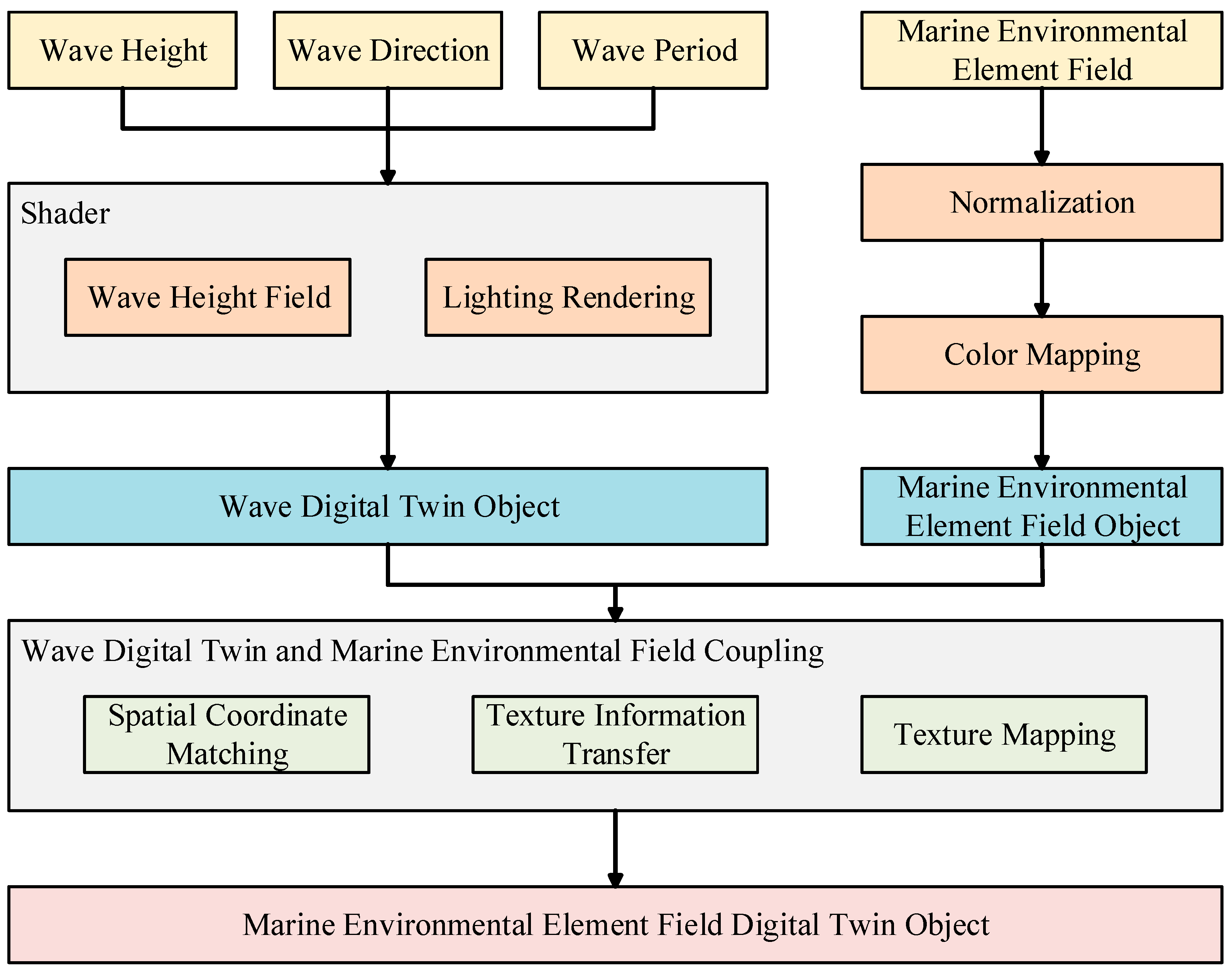
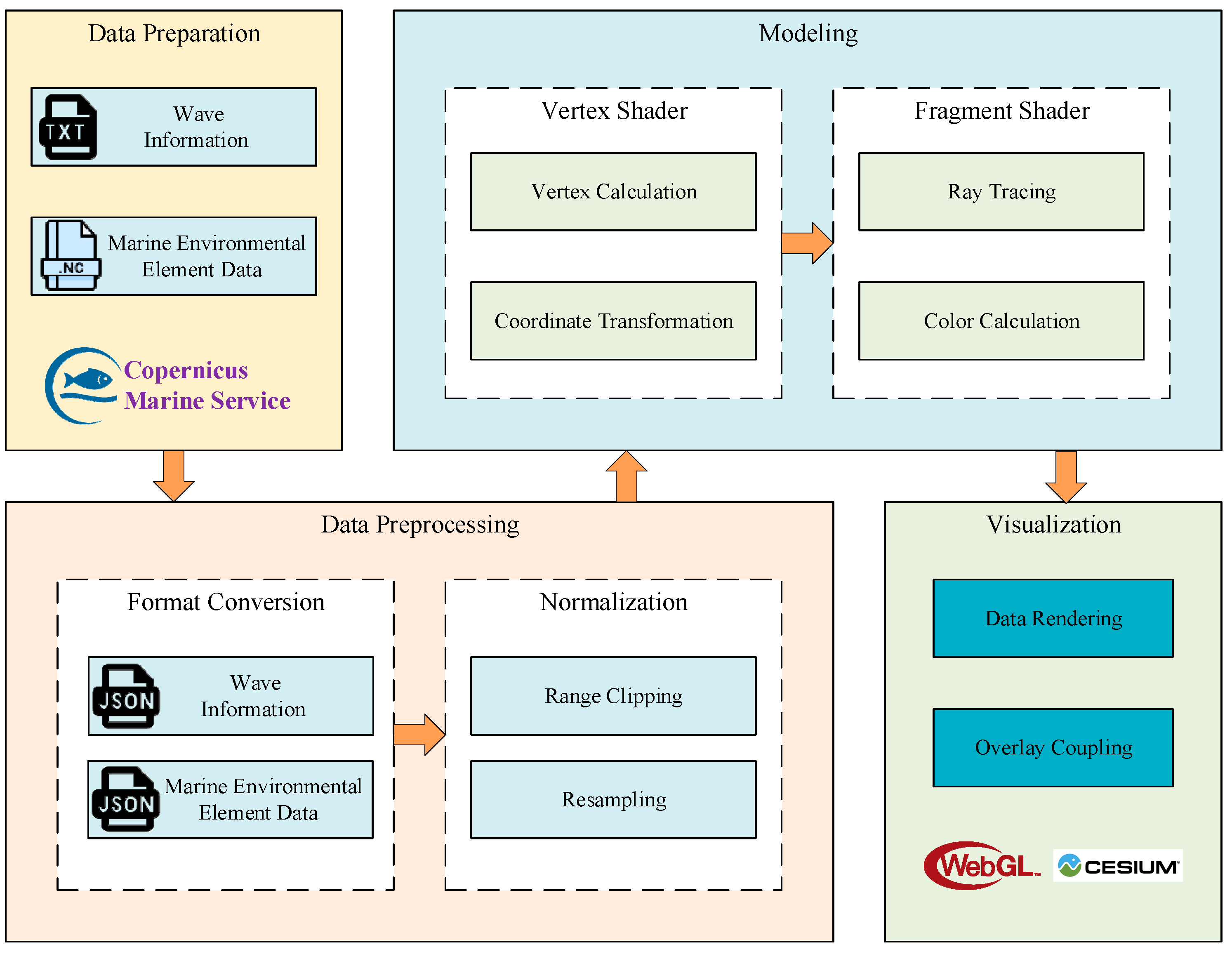
3.1. Research Framework
3.2. Wave Twin Object Modeling
3.2.1. Wave Height Field Modeling
3.2.2. Surface Lighting Rendering
3.3. Ocean Environmental Element Field Object Modeling
3.3.1. Ocean Environmental Element Field Representation Model
3.3.2. Normalization and Color Mapping
3.4. Overlay Coupling
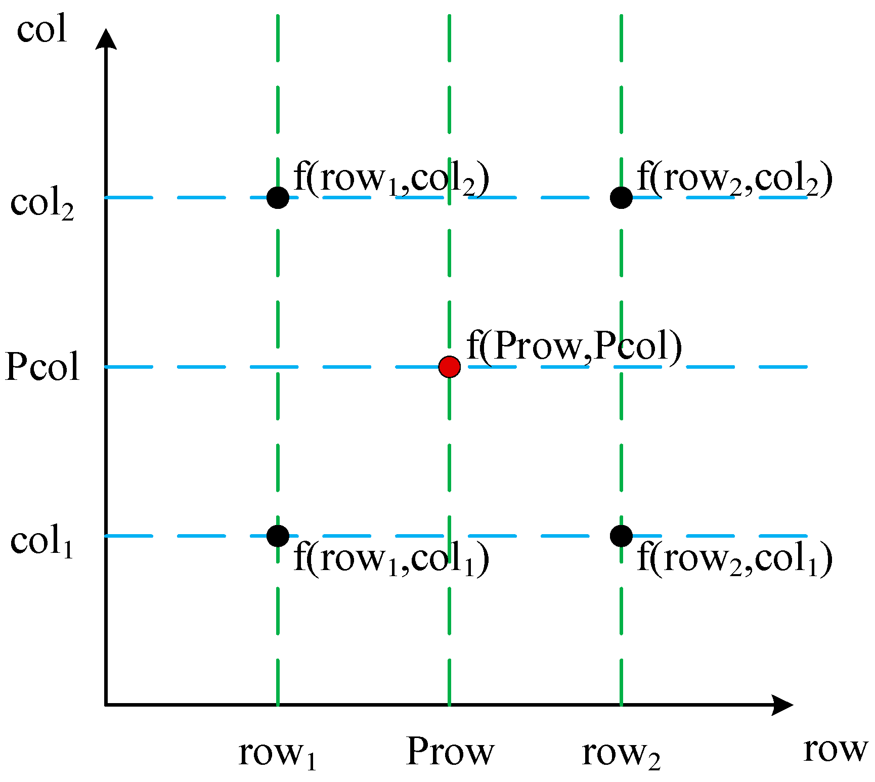
3.4.1. Spatial Coordinate Matching
3.4.2. Texture Information Transfer and Texture Mapping
4. Experiments and Results
4.1. Study Area and Dataset
4.2. Modeling
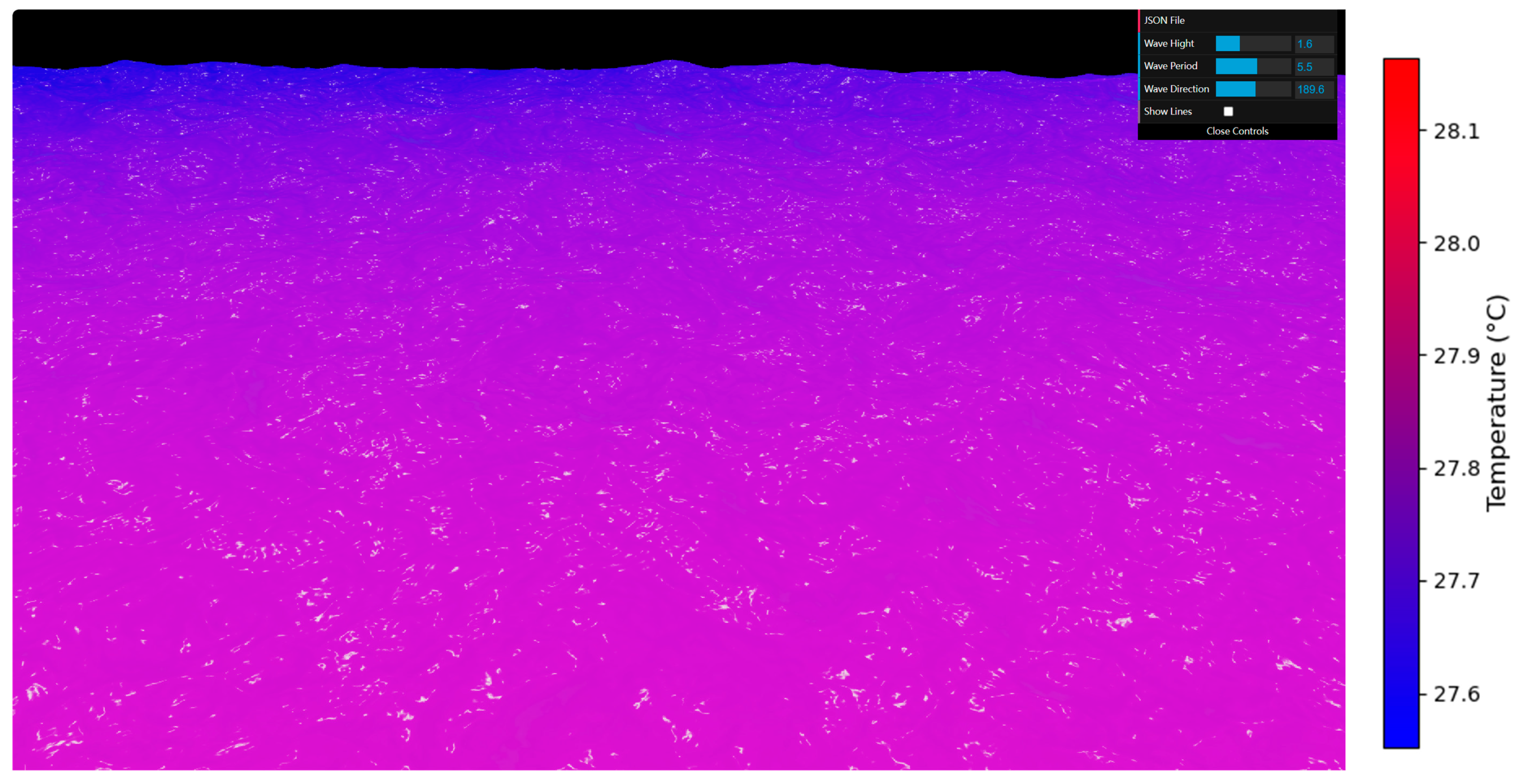
4.3. Visualization
5. Conclusions
Author Contributions
Funding
Institutional Review Board Statement
Informed Consent Statement
Data Availability Statement
Conflicts of Interest
References
- Tian, F.; Mao, Q.; Zhang, Y.; Chen, G. i4Ocean: Transfer function-based interactive visualization of ocean temperature and salinity volume data. Int. J. Digit. Earth 2021, 14, 766–788. [Google Scholar] [CrossRef]
- Chen, G.; Yang, J.; Huang, B.; Ma, C.; Tian, F.; Ge, L.; Xia, L.; Li, J. Toward digital twin of the ocean: From digitalization to cloning. Intell. Mar. Technol. Syst. 2023, 1, 3. [Google Scholar] [CrossRef]
- Xu, J.; Zhao, B.; Wei, S.; Li, G.; Xu, J.; Xiao, X. Discussion and practice on visualization technology of digital twin watershed. Express Water Resour. Hydropower Inf. 2023, 44, 127–130. [Google Scholar] [CrossRef]
- Vasilijevic, A.; Brönner, U.; Dunn, M.; Valle, G.G.; Fabrini, J.; Jones, R.S.; Bye, B.L.; Mayer, I.; Berre, A.; Ludvigsen, M.; et al. A Digital Twin of the Trondheim Fjord for Environmental Monitoring—A Pilot Case. J. Mar. Sci. Eng. 2024, 12, 1530. [Google Scholar] [CrossRef]
- Qiao, Y.; Shan, H.; Wang, H.; Zhu, C.; Sun, Z.; Jia, Y. Implementation and application of digital twin-based visualization technology for spatial and temporal variation of seafloor suspensions. Haiyang Xuebao 2023, 45, 166–177. [Google Scholar]
- Zhao, L.; Jiang, X.; Hong, Y.; Sun, M.; Wang, Y.; Kang, L.; Cao, L. Smart ocean digital twin technology and its application. Sci. Technol. Rev. 2024, 42, 91–101. [Google Scholar]
- Han, Y.; Huang, J.; Ma, C.; Yang, J.; Chen, G. Research on Key Technologies and Implementation on Virtual Marine Environment Simulation. Period. Ocean. Univ. China 2023, 53, 111–117. [Google Scholar] [CrossRef]
- Fu, J.; Huang, F.X.; Gao, W.; Yin, B.G.; Li, L.H. A Research Review on Wave Modeling and Simulation Methods in Marine Environment. In Proceedings of the 2019 IEEE International Conference on Mechatronics and Automation (ICMA), Tianjin, China, 4–7 August 2019; pp. 303–307. [Google Scholar] [CrossRef]
- Duan, X.; Liu, J.; Wang, X. Real-Time Wave Simulation of Large-Scale Open Sea Based on Self-Adaptive Filtering and Screen Space Level of Detail. J. Mar. Sci. Eng. 2024, 12, 572. [Google Scholar] [CrossRef]
- Kellomäki, T. Fast Water Simulation Methods for Games. Comput. Entertain. (CIE) 2017, 16, 1–14. [Google Scholar] [CrossRef]
- Jeschke, S.; Hafner, C.; Chentanez, N.; Macklin, M.; Müller-Fischer, M.; Wojtan, C. Making Procedural Water Waves Boundary-aware. Comput. Graph. Forum 2020, 39, 47–54. [Google Scholar] [CrossRef]
- Stomakhin, A.; Selle, A. Fluxed animated boundary method. ACM Trans. Graph. (TOG) 2017, 36, 1–8. [Google Scholar] [CrossRef]
- Kryachko, Y.A. Sea surface visualization in world of warships. In Proceedings of the International Conference on Computer Graphics and Interactive Techniques, ACM, Anaheim, CA, USA, 24–28 July 2016. [Google Scholar]
- Hu, X.; Yang, H.; Wan, Y. Research and implementation of screen space based ocean simulation. Comput. Eng. Des. 2015, 36, 452–457. [Google Scholar] [CrossRef]
- Chang, Z.; Han, F.; Sun, Z.; Gao, Z.; Wang, L. Three-dimensional dynamic sea surface modeling based on ocean wave spectrum. Acta Oceanol. Sin. 2021, 40, 38–48. [Google Scholar] [CrossRef]
- Li, T.; Ji, M.; Jin, F.; Zhang, J.; Sun, Y. Research on ocean wave simulation based on the method of combining smoothed particle hydrodynamics with marching cubes algorithm. J. Geo-Inf. Sci. 2017, 19, 161–166. [Google Scholar]
- English, R.E.; Qiu, L.; Yu, Y.; Fedkiw, R. Chimera grids for water simulation. In Proceedings of the Computer Animation, Anaheim, CA, USA, 19–21 July 2013. [Google Scholar]
- Nielsen, M.B.; Söderström, A.; Bridson, R. Synthesizing waves from animated height fields. ACM Trans. Graph. (TOG) 2013, 32, 1–9. [Google Scholar] [CrossRef]
- Han, X.; Liu, J.; Tan, B.; Duan, L. Design and Implementation of Smart Ocean Visualization System Based on Extended Reality Technology. J. Web Eng. 2021, 20, 557–574. [Google Scholar] [CrossRef]
- Guo, X.; Zhu, J.; Wan, J.; Wang, X. 3D visualization of marine environmental elements based on Cesium. Mar. Sci. 2021, 45, 130–136. [Google Scholar]
- Li, W.; Liang, C.; Yang, F.; Ai, B.; Shi, Q.; Lv, G. A Spherical Volume-Rendering Method of Ocean Scalar Data Based on Adaptive Ray Casting. ISPRS Int. J. Geo-Inf. 2023, 12, 153. [Google Scholar] [CrossRef]
- Qin, R.; Feng, B.; Xu, Z.; Zhou, Y.; Liu, L.; Li, Y. Web-based 3D visualization framework for time-varying and large-volume oceanic forecasting data using open-source technologies. Environ. Model. Softw. 2021, 135, 104908. [Google Scholar] [CrossRef]
- Lv, T.; Fu, J.; Li, B. Design and Application of Multi-Dimensional Visualization System for Large-Scale Ocean Data. ISPRS Int. J. Geo-Inf. 2022, 11, 491. [Google Scholar] [CrossRef]
- Fan, Y.; Lv, X.; Zhang, J.; Wang, Y.; Zhang, X. Research and realization of flow field dynamic visualization based on geometric shader. Comput. Eng. Appl. 2019, 55, 157–161. [Google Scholar]
- Fan, D.; Liang, T.; He, H.; Guo, M.; Wang, M. Large-Scale Oceanic Dynamic Field Visualization Based on WebGL. IEEE Access 2023, 11, 82816–82829. [Google Scholar] [CrossRef]
- Li, R. Dynamic 3-D Visualization System of Sea Flow Field Based on Virtual Reality Technology in the Environment of Internet of Things. J. Test. Eval. 2024, 52, 1542–1552. [Google Scholar] [CrossRef]
- Shi, Q.; Ai, B.; Wen, Y.; Feng, W.; Yang, C.; Zhu, H. Particle System-Based Multi-Hierarchy Dynamic Visualization of Ocean Current Data. ISPRS Int. J. Geo-Inf. 2021, 10, 667. [Google Scholar] [CrossRef]
- Wang, P.; Wang, F.; Zhang, Y.; Zhang, B.; Poon, T.C. Improved rapid algorithm for continuous shading based on the fully analytical polygon-based method. Opt. Express 2024, 32, 37418–37433. [Google Scholar] [CrossRef] [PubMed]
- Zheng, H.; Chen, J.; Qin, X.; Ma, J.; Zhang, M. Visualization Method of Vertical Profile for Meteorological Multi-element Data. J. Chin. Comput. Syst. 2021, 42, 2350–2355. [Google Scholar]
- Le Traon, P.Y.; Reppucci, A.; Alvarez Fanjul, E.; Aouf, L.; Behrens, A.; Belmonte, M.; Bentamy, A.; Bertino, L.; Brando, V.E.; Kreiner, M.B.; et al. From Observation to Information and Users: The Copernicus Marine Service Perspective. Front. Mar. Sci. 2019, 6, 234. [Google Scholar] [CrossRef]
- Xi, H.; Losa, S.N.; Mangin, A.; Soppa, M.A.; Garnesson, P.; Demaria, J.; Liu, Y.; d’Andon, O.H.F.; Bracher, A. Global retrieval of phytoplankton functional types based on empirical orthogonal functions using CMEMS GlobColour merged products and further extension to OLCI data. Remote Sens. Environ. 2020, 240, 111704. [Google Scholar] [CrossRef]


| Hardware | Software |
|---|---|
| CPU: Intel(R)Core(TM) i7-13700H | OS: Windows 11 |
| RAM: 16 GB | Browser: Edge 133.0.3065.82 |
| GPU: NVIDIA GeForce GTX 4060 | Tools: VS Code 1.97, Cesium 1.116 |
| Attribute | Wave Dataset | CMEMS Dataset |
|---|---|---|
| Format | TXT | NetCDF4 |
| Spatial resolution | 0.5° × 0.5° | 0.083° × 0.083° |
| Time resolution | 6 h | 1 month |
| Space range | 111°5′–112°0′ E; 16°5′–17°0′ N | 180° W–180° E; 89° S–90° N |
| Dimension | 1 | 4320 × 2041 |
Disclaimer/Publisher’s Note: The statements, opinions and data contained in all publications are solely those of the individual author(s) and contributor(s) and not of MDPI and/or the editor(s). MDPI and/or the editor(s) disclaim responsibility for any injury to people or property resulting from any ideas, methods, instructions or products referred to in the content. |
© 2025 by the authors. Licensee MDPI, Basel, Switzerland. This article is an open access article distributed under the terms and conditions of the Creative Commons Attribution (CC BY) license (https://creativecommons.org/licenses/by/4.0/).
Share and Cite
Li, L.; Wu, S.; Xue, C.; Ma, Y.; Qin, Q. Research on Visualization Methods for Marine Environmental Element Fields in Twin Spaces. J. Mar. Sci. Eng. 2025, 13, 449. https://doi.org/10.3390/jmse13030449
Li L, Wu S, Xue C, Ma Y, Qin Q. Research on Visualization Methods for Marine Environmental Element Fields in Twin Spaces. Journal of Marine Science and Engineering. 2025; 13(3):449. https://doi.org/10.3390/jmse13030449
Chicago/Turabian StyleLi, Lianwei, Shiyu Wu, Cunjin Xue, Yingying Ma, and Qunce Qin. 2025. "Research on Visualization Methods for Marine Environmental Element Fields in Twin Spaces" Journal of Marine Science and Engineering 13, no. 3: 449. https://doi.org/10.3390/jmse13030449
APA StyleLi, L., Wu, S., Xue, C., Ma, Y., & Qin, Q. (2025). Research on Visualization Methods for Marine Environmental Element Fields in Twin Spaces. Journal of Marine Science and Engineering, 13(3), 449. https://doi.org/10.3390/jmse13030449