Trajectory Compression Algorithm via Geospatial Background Knowledge

Abstract

The maritime traffic status is monitored through the Automatic Identification System (AIS) installed on vessels. AIS data record the trajectory of each ship. However, due to the short sampling interval of AIS data, there is a significant amount of redundant data, which increases storage space and reduces data processing efficiency. To reduce the redundancy within AIS data, a compression algorithm is necessary to eliminate superfluous points. This paper presents an offline trajectory compression algorithm that leverages geospatial background knowledge. The algorithm employs an adaptive function to preserve points characterized by the highest positional errors and rates of water depth change. It segments trajectories according to their distance from the shoreline, applies varying water depth change rate thresholds depending on geographical location, and determines an optimal distance threshold using the average compression ratio score. To verify the effectiveness of the algorithm, this paper compares it with other algorithms. At the same compression ratio, the proposed algorithm reduces the average water depth error by approximately 99.1% compared to the Douglas–Peucker (DP) algorithm, while also addressing the common problem of compressed trajectories potentially intersecting with obstacles in traditional trajectory compression methods.

1. Introduction

In recent years, the volume of ship trajectory data has increased significantly, with more vessels being equipped with an Automatic Identification System (AIS). An AIS is a wireless communication technology system designed for the automatic identification and positioning of ships. According to regulations set by the International Maritime Organization (IMO), it is mandatory for ships to install AIS transceivers [1]. IS systems gather and transmit ship identification information, navigation statuses, and other pertinent data through satellite and ground station communications. The widespread adoption of onboard AIS equipment, coupled with advancements in data reception and storage, has led to an accumulation of vast amounts of ship AIS data and a rich record of vessel trajectories. There is now significant interest in extracting useful information from these large-scale, dynamic, complex, and often chaotic datasets to analyze and predict maritime behavior [2]. AIS data have been widely used in vessel trajectory prediction [3], maritime traffic pattern recognition [4], the detection and analysis of ship behavior [5,6], extraction of maritime routes [7], analysis of maritime traffic safety [8,9,10], and evaluation of ship pollutant emissions [11,12].

AIS data report navigation information every 2 to 10 s or every 3 min when the ship is at anchor [13]. The dynamic information includes the ship’s position (longitude and latitude), timestamp, Course Over Ground (COG), Speed Over Ground (SOG), true heading, etc. [14]. For a typical merchant ship that sails 24 h a day and sends an AIS message every 5 s on average, approximately 17,280 records would be generated per day. In busy ports or waterways accommodating thousands of vessels, the daily volume of generated AIS data can reach into the millions or even hundreds of millions of records. Consequently, the overall volume of AIS data is exceedingly large. Despite this high volume, the frequency of changes in speed and heading during navigation is much lower than the recording and transmission rate of AIS data. As a result, there are numerous redundant points within the trajectory data. Removing these redundant points and retaining only a subset does not significantly affect the representation of the vessel’s path. By eliminating some of this redundant information, storage space can be reduced, which is crucial for enhancing data processing efficiency and reducing storage costs. Compressed AIS trajectory data facilitate subsequent analysis and applications. Researchers employ trajectory compression algorithms to remove redundant points while preserving those that capture key trajectory features. The remaining points still accurately represent the original trajectory. The objective of trajectory compression is to substantially reduce the amount of data while minimizing information loss.

To address the issues mentioned above, this paper proposes a trajectory compression algorithm via geospatial background knowledge. The method presented in this paper is divided into four steps, as shown in Figure 1: the first step is data cleaning, which ensures the accuracy of the data through coordinate transformation and correction of abnormal values; the second step is trajectory segmentation based on distance from the shoreline; the third step is describing the trajectory compression algorithm via geospatial background knowledge; and the fourth step is selecting an appropriate threshold for the water depth change rate.

The remaining sections of this paper are organized as follows: In Section 2, we introduce the current research methods of trajectory compression algorithms; In Section 3, we introduce the method proposed in this paper; Section 4 verifies the feasibility of the proposed algorithm in this paper through the compression of AIS data from Ningbo-Zhoushan Port and comparisons with other algorithms, as well as visual analysis; Section 5 draws conclusion and future plans.

2. Literature Review

2.1. Theoretical Research on Trajectory Compression

Trajectory compression algorithms can be classified into two categories: those that preserve trajectory shape features and those that preserve trajectory semantic features. Spatio-temporal information is the primary data contained within a trajectory, allowing compression algorithms based on this information to retain the shape characteristics of the trajectory. Semantic information refers to the relationship between objects and their environment, and considering this semantic context enables compressed trajectories to retain more inherent information about the trajectory itself.

The Douglas–Peucker (DP) algorithm [15] is the most classic algorithm, which is a global compression algorithm that uses perpendicular Euclidean distance for compression. The DP algorithm calculates the perpendicular distance of each intermediate point to the line segment formed by the start and end points. It identifies the point with the maximum distance. If this maximum distance exceeds the threshold, the point is retained, and the trajectory is split at this point. This process is recursively applied to each segment until the maximum distance in all segments is below the threshold. It is able to preserve the shape features of the trajectory, ultimately ensuring that the distance between the original trajectory points and the compressed trajectory does not exceed a set threshold. However, since the DP algorithm cannot preserve the temporal features of the trajectory, Meratnia et al. [16] proposed the Top-Down Time Ratio (TD-TR) algorithm, which replaces the perpendicular Euclidean distance with the Synchronized Euclidean Distance (SED). These algorithms require recalculating the error each time a point with the maximum distance error is retained, thus consuming more time. The Scan–Pick–Move (SPM) algorithm was proposed by Singh et al. [17], and its basic idea is to connect the first and last points and then sequentially remove points whose perpendicular Euclidean distance exceeds the threshold. This algorithm has a lower time complexity compared to the DP algorithm, but it has a larger error.

Compared to offline algorithms, online algorithms preserve more feature points. Online algorithms remove redundant data from trajectories as they emerge, avoiding unnecessary data transmission, improving data storage, and reducing memory space. The main online compression algorithms include the sliding window (SW) algorithm [16], whose basic idea is to set a sliding window starting from the initial point. The window always contains three consecutive points, and if the SED error of the middle point is less than a set threshold, it is removed and the next point is added to the sliding window. If the error is greater than the threshold, the point is retained and becomes the new starting point of the sliding window. The Open Window (OPW) algorithm [18] has a similar principle: it sets a window at the initial point and sequentially adds subsequent points to the window. When there is a point in the window whose SED to the line connecting the first and last points in the window exceeds the threshold, that point is retained and becomes the new starting point. The Spatial Quality Simplification Heuristic (SQUISH) algorithm [19] calculates the importance of each point and removes the least important points.

While the above algorithms primarily focus on preserving the shape features of trajectories, they do not consider other semantic features, resulting in significant changes in semantic information for some points. To better preserve the semantic information of trajectories, Long et al. [20] proposed the DPTS algorithm, which significantly reduces trajectory data while keeping the direction error within a threshold. Meratnia et al. introduced a velocity-preserving trajectory simplification method that compresses trajectories by retaining points where the velocity change exceeds a threshold. Yang et al. [21] proposed a trajectory simplification method that considers speed loss. To preserve speed, the speed-enrichment component employs a data-enrichment strategy to enhance simplification where the loss of speed exceeds a given tolerance. Lin et al. [22] presented the Adaptive Trajectory Simplification (ATS) algorithm, which segments trajectories based on velocity intervals and uses the Minimum Description Length (MDL) concept to infer the optimal distance threshold for each interval, enabling the trajectory to adaptively select thresholds. Gao et al. [23] proposed an algorithm for compressing trajectory data based on the ship’s navigation state and acceleration variation. This algorithm can maintain very low emission calculation errors. Ma et al. [24] propose a direction-preserved vessel trajectory compression method based on Open Window, which also reduces the compression time. Liu et al. [25] adopted a trajectory compression algorithm that considers both speed and heading.

2.2. Research on Ship Trajectory Compression

The main issue with compression algorithms that aim to preserve trajectory shape features is the need to set an appropriate threshold. For example, Liu et al. [25] have adopted fixed values as the compression threshold for trajectories. However, due to the varying motion characteristics of ships, a fixed threshold cannot be suitable for all trajectories. The choice of threshold affects both the compression rate and the compression quality of the trajectory. To select a reasonable threshold, Zhang et al. [26] simplified shipping trajectories using the DP algorithm and set the threshold at 0.8 times the ship’s length, achieving a compression rate of 98.25% while ensuring that the simplified trajectory points remain within a safe range of the original trajectory points. Tang et al. [27] improved the DP algorithm by first filtering out trajectories with minor shape changes, reducing computation time. Secondly, they adaptively changed the compression distance threshold based on the critical threshold of the trajectory points, improving compression accuracy. Xie et al. [5] select the threshold of the penultimate stable phase as the final compression threshold for each trajectory. Huang et al. [28] proposed an average compression score indicator to determine the optimal compression threshold.

The above research has made the selection of thresholds more reasonable, but did not consider semantic information like ship speed and course during compression, leading to significant changes in such semantic information for some points. To address this issue, some studies have proposed improvements to these algorithms. Zhu et al. [29] introduced a ship trajectory compression algorithm that considers maneuvering patterns. It retains points exceeding the course change threshold and speed change threshold and applies a sliding window method for compression. Compared to other algorithms, this method achieves higher computational speed. Wei et al. [30] adopted the strategy of calculating the standard deviation of speed and course information for each trajectory to identify characteristic points of speed and course and selected an appropriate threshold coefficient. This method can adaptively preserve course and speed information for each trajectory. Due to considering more semantic information, the compression effect of these algorithms is slightly reduced. Zhang et al. [14] adopted an improved DOTS algorithm to preserve the position, speed, and course characteristics of trajectories. Experiments showed that under the same compression rate, this algorithm performs better in preserving distance, speed, and course information compared to other algorithms. Zhou et al. [31] improved the DP algorithm by using a multi-objective fitness function that considers spatial characteristics, heading, and speed comprehensively, enabling the preservation of more semantic information while maintaining a high compression rate.

While research has already considered a ship’s heading and speed information, few studies have taken geographical information into account, which is important considering it can avoid having compressed trajectories cross obstacles. Lee et al. [32] considered the influence of geographical factors, as compressed trajectories may intersect with obstacles. They adopted a polygon map random (PMR) quadtree to consider coastal topographic information. When a compressed trajectory is found to intersect with an obstacle, the two points before and after the intersection are recompressed to ensure that the compressed trajectory accurately avoids the obstacle. Yan et al. [33] considered that the distance between a trajectory point and the shoreline can affect the choice of threshold, and dynamically adjusted the threshold during the trajectory compression process based on the minimum distance from the point to the shoreline.

Currently, most trajectory compression algorithms that consider semantic information focus on preserving ship speed and course details, but there is limited research on ship trajectory compression that includes water depth retention. As ships are maritime transportation vehicles, the water depths they encounter can vary significantly during navigation. Variations in water depth greatly impact route planning and safety when ships navigate at sea. Traditional trajectory compression algorithms typically prioritize retaining data such as speed and heading but overlook the critical factor of water depth. Given that ships need to avoid shallow waters to prevent grounding and identify potential navigational hazards (such as shipwrecks, reefs, and navigation markers), water depth information is particularly crucial. Moreover, accurate water depth data aid in optimizing routes, improving fuel efficiency, and ensuring navigational safety. Therefore, when compressing ship trajectories, retaining water depth information not only enhances the accuracy of the compressed trajectory but also improves the safety and reliability of navigation.

3. Algorithm Description

The TD-TR algorithm minimizes the SED error and is capable of preserving the spatio-temporal features of trajectories. However, since the algorithm does not take geographical background information into account, the compressed trajectories fail to retain water depth information and may traverse obstacles. To address this issue, this paper enhances the TD-TR algorithm, enabling it to preserve water depth information and accurately avoid obstacles.

3.1. Data Cleaning

Vessel trajectories are identified by the Maritime Mobile Service Identity (MMSI) number of the vessel. However, due to improper operation, there are instances where the same MMSI number is shared by multiple vessels, resulting in trajectory jumps between different positions at a given moment. Additionally, ship trajectory data can contain errors caused by abnormal or missing signals. Trajectory cleaning is performed to remove these error points and ensure that each vessel corresponds to a unique MMSI number.

The data cleaning algorithm adopted in this paper follows the approach of Yan et al. [33]. Firstly, the raw data are segregated based on the MMSI number and divided into multiple files in chronological order. Each file is processed sequentially by iterating through all the trajectory points. When the distance or time interval between two consecutive points exceeds a predefined threshold, the starting point of this interval is considered as the beginning of a new segment for the same MMSI number. If subsequent trajectory points have a distance or time interval less than the threshold from this point, they are included in the same file. Considering the possibility of signal loss, the time threshold and distance threshold are set to 10 min and 0.5 nautical miles, respectively.

The sliding window method is adopted to detect outliers in the trajectory. By calculating the average and standard deviation of speed and acceleration of three consecutive points within the window [33], if the speed or acceleration of a subsequent point falls outside this range, it is considered an outlier. The trajectory is scanned both in forward and backward order, and if a point is deemed an outlier in both directions, it is finally identified as an outlier. After the outliers are removed, the rectified position is calculated based on the neighboring normal points using the linear interpolation method.

3.2. Trajectory Segmentation Based on Distance from Shoreline

K-means is a widely used unsupervised learning algorithm designed to partition a dataset into k clusters, where each cluster is represented by the mean value of its member points. The goal is to minimize the sum of squared distances between data points and their respective cluster centroids. In this paper, the K-means clustering algorithm is applied for trajectory segmentation, dividing the trajectory into k clusters based on the distances of trajectory points from the shoreline.

The Elbow Method is a widely used technique for determining the optimal number of clusters in K-means clustering. It involves observing how the Within-Cluster Sum of Squares (WCSS), which measures cluster compactness by calculating the sum of squared distances from each point to its cluster centroid, changes as the value of k increases. Typically, as k increases, WCSS decreases because more clusters allow data points to be closer to their centroids. However, excessively high values of k can lead to overfitting. The core idea of the Elbow Method is to plot k against the corresponding WCSS. Ideally, this plot will show a curve where the rate of decrease in WCSS slows down significantly at a certain value of k, forming an “elbow”. The k value at this elbow point is considered optimal as it represents the point where the marginal benefit of adding more clusters diminishes, thus avoiding unnecessary complexity.

Given the heterogeneity of geographic information, water depth tends to be shallower near the shoreline and deeper further away. Therefore, different thresholds for water depth variation rates should be adopted for trajectories in different geographic locations. This study utilizes the K-means clustering algorithm to determine distinct distance intervals based on the distances between trajectory points and the shoreline. We employ the Elbow Method to determine the optimal number of clusters. By incrementally increasing the number of clusters k and observing the changes in WCSS, we assess the clustering performance. As shown in Figure 2, through multiple experimental analyses, when k is set to 4, we observe that the reduction in WCSS begins to slow down significantly. This indicates that the marginal benefit of adding more clusters for improving clustering quality is rapidly diminishing. More importantly, at k = 4, the trajectories can be effectively divided into four groups: near, medium, far, and very far, corresponding to the intervals [0, 8258], [8258, 22,100], [22,100, 40,266], and [40,266, 81,520], respectively. This not only balances model complexity and clustering accuracy but also avoids overfitting due to too many clusters. Additionally, choosing k = 4 is based on an understanding and consideration of actual marine environmental characteristics. Four intervals can adequately reflect the natural gradient from shallow coastal waters to deeper oceanic regions, meeting the needs of data analysis while ensuring the interpretability and practicality of the results. Therefore, considering all these factors, k = 4 was ultimately selected as the optimal number of clusters.

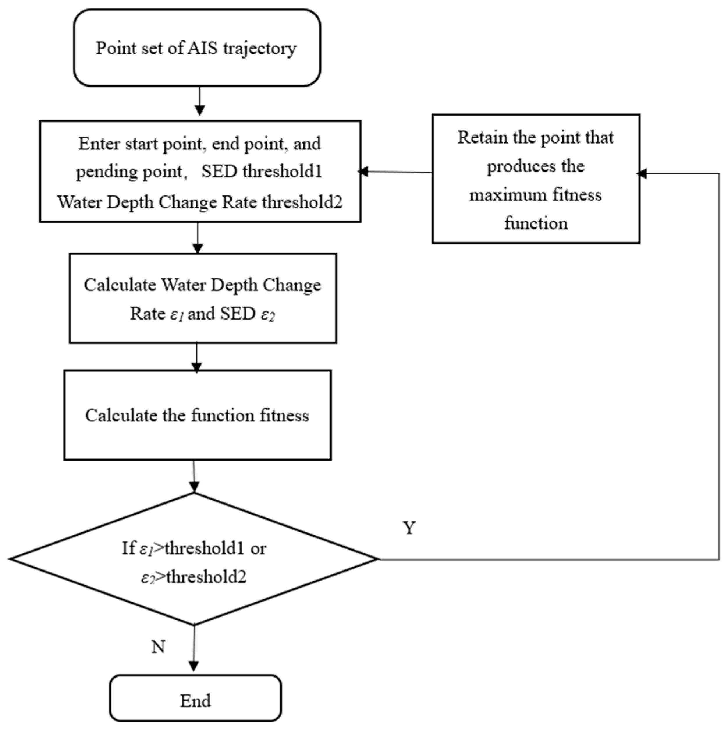
3.3. Trajectory Compression Algorithm via Geospatial Background Knowledge

In this paper, the SED is used as the distance error, as shown in Figure 3. There are three consecutive points in chronological order: P₁(x₁, y₁, t₁), P₂(x₂, y₂, t₂), and P3(x₃, y₃, t₃), where x and y represent the horizontal and vertical coordinates of the points, respectively, and t is the timestamp of the point. Point P’₂ is the synchronized time point, and the Euclidean distance between P₂ and P’₂ is the SED, which is presented as follows:

$${\mathrm{x}}_2^{\prime }=\left(\begin{array}{c}{\mathrm{x}}_3-{\mathrm{x}}_1\end{array}\right){\displaystyle \frac{{\mathrm{t}}_2 - {\mathrm{t}}_1}{{\mathrm{t}}_3 - {\mathrm{t}}_1}}$$

(1)

$${\mathrm{y}}_2^{\prime }=\left(\begin{array}{c}{\mathrm{y}}_3-{\mathrm{y}}_1\end{array}\right){\displaystyle \frac{{\mathrm{t}}_2 - {\mathrm{t}}_1}{{\mathrm{t}}_3 - {\mathrm{t}}_1}}$$

(2)

$${\mathrm{SED}}_2=\sqrt{{\left(\begin{array}{c}{\mathrm{x}}_2^{\prime }-{\mathrm{x}}_2\end{array}\right)}^2{+\left(\begin{array}{c}{\mathrm{y}}_2^{\prime }-{\mathrm{y}}_2\end{array}\right)}^2}$$

(3)

The DP algorithm is a trajectory compression algorithm aimed at minimizing the perpendicular Euclidean distance between points. In contrast, the TD-TR algorithm aims to minimize the SED error and preserve the spatio-temporal features of trajectories. Unlike the traditional DP algorithm, TD-TR not only considers spatial information but also pays special attention to temporal information to ensure that compressed trajectories are as close as possible to the original trajectories in both time and space. Calculating the SED error requires determining synchronized time points, which involves more computational effort compared to calculating perpendicular Euclidean distances. As a result, under the same compression rate, the TD-TR algorithm consumes more time than the DP algorithm.

AIS data contain positional information for trajectories but do not include water depth information. To calculate the water depth for each trajectory point, a nearest-point matching method is employed. The Electronic Navigation Chart (ENC) database includes both positional coordinates and water depth information. By finding the nearest location point in the ENC to the target point from the AIS data, the water depth of that nearest point is assigned to the target point. For non-navigable areas such as land, navigation markers, shipwrecks, and reefs, the water depth at their boundaries is set to 0. When the matched water depth information for a target point is 0, it indicates that the target point is either very close to an obstacle or within an obstacle.

Due to geographic heterogeneity, in shallow water areas, for example, if the water depth of an original trajectory point is 10 m and the compressed water depth is 20 m, the water depth error is 10 m, which is 1 times the original water depth. However, when the original point has a water depth of 100 m and the compressed point has a water depth of 90 m, the water depth error is also 10 m, but the latter’s water depth error is only 0.1 times the original water depth. This paper adopts the ratio of the difference in water depth before and after compression to the original water depth as an evaluation index for water depth error.

The basic idea of the TD-TR algorithm is to find the point with the maximum SED error as the segmentation point each time. However, the goal of this paper is to identify a segmentation point that maximizes both the water depth change rate and the SED error. It is important to note that the point with the maximum water depth variation rate may not coincide with the point having the maximum distance error. Therefore, this paper adopts a fitness function that considers both factors to determine the optimal segmentation point. Given that the units and magnitudes of water depth error and distance error can differ significantly, normalization is required. Water depth errors and distance errors are calculated separately, and the min–max normalization method is used to map these errors to a range of [0, 1]. The transformation equation is presented as follows:

$$\mathrm{F}={\displaystyle \frac{\mathrm{f} - \min }{\max - \min }}$$

(4)

where max and min represent the maximum and minimum values in the set, f is the original objective function, and F is the normalized objective function.

The adaptation function fitness is calculated as follows:

$$\mathrm{fitness}=\mathsf{\alpha } \times \mathrm{d}+\mathsf{\beta } \times \mathsf{\eta }$$

(5)

$$\mathsf{\alpha }+\mathsf{\beta }=1$$

(6)

where d is the normalized distance error, and η is the normalized rate of water depth change. α and β are weight factors for the distance error and the water depth change rate, respectively, which can be adjusted according to user requirements. In this paper, both α and β are set to 0.5.

As shown in Figure 4, the steps of the algorithm in this paper are as follows.

Set the thresholds for the water depth change rate and the SED error, and input the trajectory that needs to be compressed. Connect the start and end points of each trajectory segment, find the synchronized time point corresponding to each original point, and calculate the SED error and water depth change rate separately. Compute the fitness function value, and retain the maximum value as the compressed point. If either the water depth change rate or the SED error exceeds its threshold, repeat the above operations. Once both the water depth change rate and the SED error are within their respective thresholds, output the compressed trajectory. The pseudo-code for the trajectory compression algorithm using geospatial background knowledge is shown in Algorithm 1.

Algorithm 1. Trajectory Compression Algorithm via Geospatial Background Knowledge

Input: A trajectory T = {p0, p1,…, pi−1}, water depth change rate threshold1, distance threshold2. Output: Simplified trajectory points set KS Initialize KS with start point and end point Calculate the distance d from point p to the shoreline Determine threshold1 based on d ε1_values = [] ε2_values = [] for each point p in T do   Calculate Water Depth Change Rate ε1, append ε1 to ε1_values   Calculate SED ε2, append ε2 to ε2_values end for Normalize ε1 and ε2 using Equation (4) Calculate fitness using Equation (5) max_fitness_index is the index of the maximum value in fitness ε1_max = ε1_values[max_fitness_index] ε2_max = ε2_values[max_fitness_index] if ε1_max >= threshold1 or ε2_max >= threshold2 then   Add T[max_fitness_index] to KS else   break end if return KS

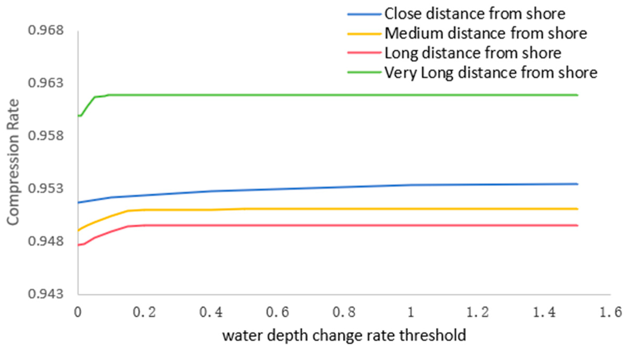
3.4. Water Depth Change Rate Threshold and Distance Threshold Selection

Generally, the greater the threshold for the water depth change rate is, the larger the error of the average water depth change rate becomes, and the higher the compression rate will be. A reasonable threshold for the water depth change rate can maintain a high compression rate while keeping the average water depth change rate relatively low. Due to the heterogeneity of geographic information, different thresholds for the water depth change rate need to be adopted for each interval. To select a reasonable compression threshold, Huang et al. [28] proposed an average compression score to balance the compression rate and length loss rate. The goal of this paper is to achieve as high a compression rate as possible while keeping the average water depth change rate error as low as possible. Therefore, this paper identifies a reasonable threshold for the water depth change rate by calculating the compression score. In this study, the distance error threshold is fixed at 50 m, and by varying the threshold for the water depth change rate, a balance is achieved between the average water depth change rate and the compression rate.

The compression rate is the ratio of the number of discarded trajectory points to the original number of trajectory points. The compression rate (CR) of all trajectories is as follows:

$$\mathrm{CR}={\displaystyle \frac{\mathrm{M}}{\mathrm{N}}}$$

(7)

where N represents the number of track points of all trajectories and M denotes the total number of discarded points.

The formula for calculating the compression score is as follows:

$$\mathrm{CS}=1 - {\displaystyle \frac{\mathrm{CR} - \mathrm{C}{\mathrm{R}}_{\mathrm{MIN}}}{\mathrm{C}{\mathrm{R}}_{\mathrm{MAX}} - \mathrm{C}{\mathrm{R}}_{\mathrm{MIN}}}}+{\displaystyle \frac{\mathrm{AWDCR} - \mathrm{AWDC}{\mathrm{R}}_{\mathrm{MIN}}}{\mathrm{AWDC}{\mathrm{R}}_{\mathrm{MAX}} - \mathrm{AWDC}{\mathrm{R}}_{\mathrm{MIN}}}}$$

(8)

where CS is the compression score; CR is the compression rate; CR_MIN and CR_MAX are the maximum compression rate and minimum compression rate, respectively; CS is the compression score; AWDCR is the average water depth change rate; AWDCR_MIN and AWDCR_MAX are the maximum average water depth change rate and minimum average water depth change rate, respectively.

By calculating the compression score, it is found that the score reaches its minimum when the water depth change rate thresholds are set to 0.05, 0.1, 0.1, and 0.5, respectively. This indicates a balance between the compression rate and the water depth change rate. When the trajectory is at a medium or long distance from the shoreline, changes in the average water depth variation rate and compression rate are largely consistent; therefore, these two cases can be merged into one category.

Figure 5 shows the error in the average water depth change rate for different thresholds of the water depth change rate across four scenarios. Figure 6 displays the compression rate for various thresholds of the water depth change rate in these four scenarios. As the threshold for the water depth change rate increases, both the error in the average water depth variation rate and the compression rate exhibit a trend of rapidly rising before gradually stabilizing. In the four scenarios, within the intervals of [0, 1], [0, 0.15], [0, 0.15], and [0, 0.1] for the water depth change rate threshold, significant changes occur in both the error of the average water depth change rate and the compression rate. The primary reason for this is that shallow water areas are more common near the shore, where small changes in water depth before and after compression can result in relatively large water depth change rates. Additionally, ships near the shore tend to maneuver more frequently compared to those further from the shoreline, leading to higher water depth change rates. Tracks farther away from the shoreline have deeper waters, and vessels do not frequently alter their course while navigating. When the threshold for the water depth change rate exceeds these intervals, both the compression rate and the error in the average water depth change rate tend to stabilize. Specifically, the compression rate increased by only approximately 0.2% in all four scenarios as the threshold for the water depth change rate was gradually raised from 0 to 1, indicating that the algorithm presented in this paper only needs to retain a small portion of points to preserve more water depth information.

The distance threshold is an important parameter in trajectory compression. Selecting an appropriate distance threshold is a critical step to ensure that trajectory compression can effectively reduce data volume without losing key information. Therefore, this paper identifies a reasonable distance threshold by calculating the compression score. To determine the appropriate distance threshold, this paper adopts the Average Compression Score (ACS) proposed by Huang et al. [28] to establish the compression threshold, a trajectory point set (T = {p₁, p₂, …, p_i}), the original trajectory set (TR_orginal = {T₁, T₂, …, T_n}), and the compressed trajectory set (TR_compress = {T′₁, T′₂, …, T′_n}).

The formula is as follows:

$$\left|\begin{array}{c}\mathrm{T}\end{array}\right|=\sum _{\mathrm{j}=1}^{\mathrm{i}-1}\left|{\mathrm{p}}_{\mathrm{j}}{\mathrm{p}}_{\mathrm{j}+1}\right|$$

(9)

$$\left|\begin{array}{c}\mathrm{T}\_\mathrm{b}\mathrm{a}\mathrm{s}\mathrm{e}\mathrm{l}\mathrm{i}\mathrm{n}\mathrm{e}\end{array}\right|=\left|\begin{array}{c}{\mathrm{p}}_1{\mathrm{p}}_{\mathrm{i}}\end{array}\right|$$

(10)

$$\mathrm{IALLR} ={\displaystyle \frac{\sum _{\mathrm{j}=1}^{\mathrm{n}}\left|{\mathrm{T}}_{\mathrm{j}}\right| - \sum _{\mathrm{j}=1}^{\mathrm{n}}\left|{\mathrm{T}}_{\mathrm{j}}^{\prime }\right|}{\sum _{\mathrm{j}=1}^{\mathrm{n}}\left|{\mathrm{T}}_{\mathrm{j}}\right| - \sum _{\mathrm{j}=1}^{\mathrm{n}}\left|\begin{array}{c}{\mathrm{T}\_\mathrm{baseline}}_{\mathrm{j}}\end{array}\right|}}$$

(11)

$$\mathrm{ACS}=1 - \mathrm{CR}+\mathrm{IALLR}$$

(12)

where |T| is the distance of the trajectory; |T_baseline| is the distance between the starting and ending points of the trajectory; IALLR is the improved indicator of the average length loss rate, and it can preserve the robustness of the ACS.

With the increase in the distance threshold, the ACS gradually decreases, reaching its minimum when the distance threshold is 60 m, and then gradually increases. The distance threshold is optimal when the ACS is at its smallest, as shown in Figure 7. Therefore, this paper sets the distance threshold to 60 m.

4. Experiments and Analyses

In this paper, we used AIS data from the waters near Ningbo-Zhoushan Port collected between 1 May and 7 May 2020, comprising a total of 13,627,909 data points. To validate the effectiveness of the algorithms, our proposed algorithm, which incorporates geospatial background knowledge, was compared with the DP algorithm, TD-TR algorithm, and algorithms that consider ship speed and course. Under the condition of the same compression rate, we compared the average SED error, maximum SED error, average water depth variation rate, maximum water depth variation rate, average water depth error, and maximum water depth error among these algorithms. Furthermore, a visual analysis was also conducted. All the experiments are conducted on a laptop with processer i5-9300H and RAM 8 GB. The programming language is Python 3.7.

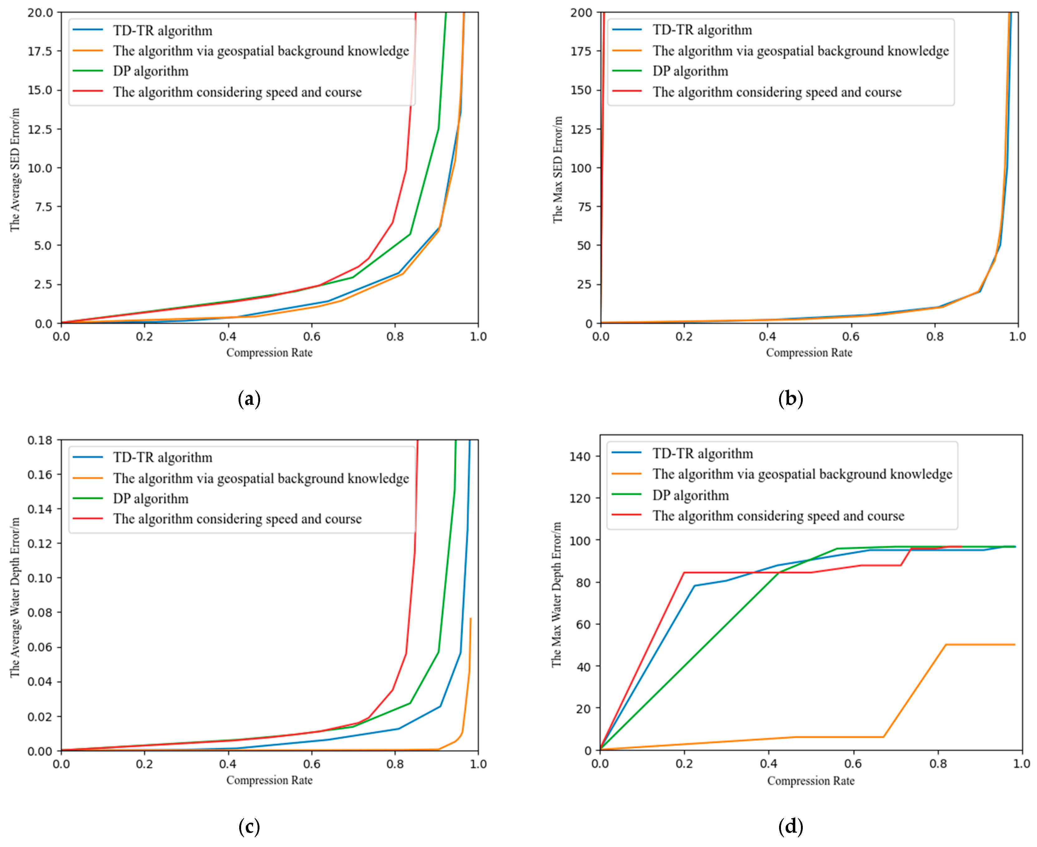
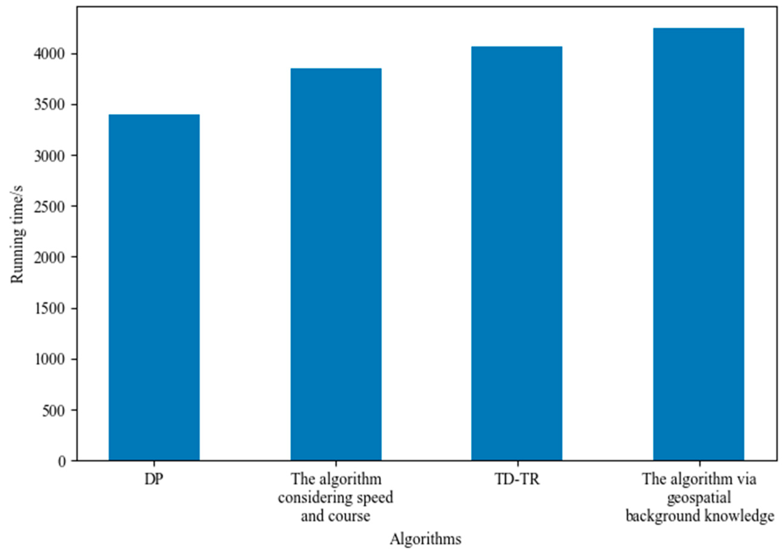
4.1. Comparison with Other Algorithms

Figure 8 shows the comparative results of different algorithms. (a), (b), (c), (d), (e), and (f) represent the average SED error, the maximum SED error, the average water depth error, the maximum water depth error, the average water depth change, and the maximum water depth change of the four algorithms under the same compression rate, respectively. Compared with the TD-TR algorithm, the proposed method exhibits a similar average SED error. Both algorithms use SED as the distance error metric, while the proposed algorithm employs a fitness function that considers both the rate of water depth change and the SED error. With the same SED error settings for both algorithms, the proposed approach retains only approximately 0.2% more points, thus resulting in similar average SED errors under the same compression rate. In comparison with the DP algorithm and the algorithm that considers ship speed and course, the proposed algorithm achieves a lower SED error under the same compression rate. This is due to the fact that the DP algorithm and the algorithm considering ship maneuvering behavior both utilize vertical Euclidean distance as the error metric for compression. However, the algorithm that takes into account ship maneuvering behavior retains more points related to speed and heading information, leading to a lower compression rate at the same error level.

It can be observed that ignoring water depth information would result in significant water depth errors. Compared with other algorithms, the average and maximum water depth errors of the proposed algorithm are much smaller. Moreover, the proposed algorithm sets a threshold for the water depth change rate, ensuring that the maximum water depth change rate does not exceed this threshold, leading to a substantial reduction in the average water depth change rate. When the compression rate exceeds 0.8, the maximum water depth error of the proposed algorithm is 50 m, whereas the maximum water depth error of other algorithms reaches 96.6 m, which is nearly double that of the proposed algorithm. The maximum water depth change rate of the proposed algorithm is 0.5, while that of other algorithms can reach up to 399, significantly higher than that of the proposed algorithm. At a compression ratio of 0.9, the average water depth change rate of the proposed algorithm is 0.003%, and the average water depth error is 0.00051 m. The average water depth change rates of the TD-TR and DP algorithms are 83 times and 183 times higher than that of the proposed algorithm, respectively, and their average water depth errors are 50 times and 111 times higher. Clearly, the proposed algorithm excels in retaining water depth information compared to other algorithms.

As shown by the curves of average water depth error and average water depth change rate in Figure 8c,e, it is evident that when the compression ratio is below 0.9, both the average water depth error and the average water depth change rate remain relatively stable. Within this range, the semantic integrity of water depth information is effectively maintained. However, once the compression ratio exceeds 0.9, these metrics exhibit a notable increase, indicating that the semantic accuracy of water depth information becomes significantly compromised. Moreover, as the compression ratio continues to increase, the adverse impact on water depth information becomes increasingly pronounced.

To evaluate the performance of the algorithms, they were tested under a uniform compression rate of 97%. As shown in Figure 9, the DP algorithm had the shortest runtime at 3399.7 s, while the TD-TR algorithm required 4060.1 s. The algorithm presented in this paper had the longest runtime at 4247.5 s, which is 25% longer than that of the DP algorithm and 4.6% longer than that of the TD-TR algorithm. The additional consideration of bathymetric information in this algorithm makes the calculations more complex, thus slightly increasing the runtime. When compressing AIS data, processing time can be reduced by optimizing data structures, simplifying computational steps, and eliminating redundant calculations.

4.2. The Validation of Visual Observation

To better demonstrate the visual effects of the proposed algorithm, the original trajectory and the compressed trajectory were plotted separately. The distance threshold for the algorithm was set to 60 m. As shown in Figure 10, the blue line represents the shoreline contour, while the green line represents the ship’s trajectory. The number of original trajectory points is 13,627,909, whereas the number of compressed trajectory points is 574,621, resulting in a compression rate of 95.78%. The average water depth error is 0.0085 m. Under the same compression rate, the average water depth errors of the TD-TR algorithm and DP algorithm are 0.0564 m and 0.302 m, respectively. The average water depth change rate is 0.000486. Under the same compression rate, the average water depth change rates of the TD-TR algorithm and DP algorithm are 0.00645 and 0.0457, respectively. The original trajectory is dense, while the compressed trajectory is relatively sparse. It can be observed that the simplified trajectory generated by the proposed algorithm is almost identical to the shape of the original trajectory, while retaining more water depth information. This allows it to accurately describe macroscopic traffic flow conditions.

Figure 11 shows the compression results of the TD-TR algorithm and the proposed algorithm for the MMSI number 413,411,600. When the trajectory is compressed using the TD-TR algorithm, the compressed trajectory passes through obstacles. Since the threshold for the water depth change rate in the proposed algorithm is set to 0.5, when a synchronized time point is close to or within an obstacle, the water depth at that point is 0 m, resulting in a water depth change rate of 1. Consequently, the compression process continues until the water depth change rate becomes less than 0.5. This demonstrates that the proposed algorithm can accurately avoid obstacles.

5. Conclusions

The AIS records a large amount of spatio-temporal information regarding ship trajectories, and to reduce its storage space, redundant information needs to be removed. To preserve the geospatial background information of these trajectories, this paper proposes a trajectory compression algorithm that considers geographical background information. In order to adapt to different geographical locations, trajectories are divided into four intervals based on their distance from the shoreline, with appropriate thresholds for water depth change rates selected for each interval. The DP algorithm is improved to better preserve the water depth information of the trajectories. Additionally, using the algorithm proposed in this paper to compress trajectories ensures that the compressed trajectories can accurately avoid obstacles. To verify the effectiveness of the algorithm, AIS data from the waters near Ningbo-Zhoushan Port were compressed, and comparisons were made with the DP algorithm, TD-TR algorithm, and algorithms considering speed and course. These comparisons included metrics such as average SED error, maximum SED error, average water depth error, maximum water depth error, average water depth change rate, and maximum water depth change rate. The experiments show that under the same compression rate, the proposed algorithm can better preserve water depth information. Through visual analysis, it is demonstrated that the algorithm can significantly reduce the number of trajectory points while maintaining the basic characteristics of the original trajectory. Consequently, through the trajectory compression algorithm proposed in this paper, the storage costs of AIS data are significantly reduced, and the efficiency of data processing is improved.

The limitation of this paper lies in the fact that the algorithm requires matching water depth with trajectory points, which consumes more time. Consequently, the processing time for this algorithm is longer compared to other algorithms. Moreover, the distance threshold used in this study is selected based on the compression ratio and remains fixed, unable to adapt to different ship trajectories. Additionally, the algorithm does not take into account the speed and heading information of ships, resulting in inferior performance in these aspects compared to other algorithms. Therefore, future research will focus on adopting more efficient indexing structures to accelerate the matching process between water depth and trajectory points or employing parallel processing techniques to reduce processing time. By using machine learning methods, we aim to adaptively adjust the distance thresholds. Furthermore, we will integrate speed, heading, and other semantic information to improve the accuracy and rationality of the compression results.

References

1. Schöller, F.E.; Enevoldsen, T.T.; Becktor, J.B.; Hansen, P.N. Trajectory prediction for marine vessels using historical ais heatmaps and long short-term memory networks. IFAC PapersOnLine 2021, 54, 83–89. [Google Scholar] [CrossRef]
2. Li, Z.C.; Liu, T.; Peng, X.; Ren, J.X.; Liang, S. An AIS-based deep learning model for multi-task in the marine industry. Ocean Eng. 2024, 293, 116694. [Google Scholar] [CrossRef]
3. Wang, S.W.; Li, Y.; Xing, H.; Zhang, Z.Y. Vessel trajectory prediction based on spatio-temporal graph convolutional network for complex and crowded sea areas. Ocean Eng. 2024, 298, 117232. [Google Scholar] [CrossRef]
4. Li, G.C.; Zhang, X.Y.; Jiang, L.L.; Wang, C.B.; Huang, R.N.; Liu, Z.S. An approach for traffic pattern recognition integration of ship AIS data and port geospatial features. Geo-Spat. Inf. Sci. 2024, 27, 1–28. [Google Scholar] [CrossRef]
5. Xie, Z.X.; Bai, X.E.; Xu, X.F.; Xiao, Y.J. An anomaly detection method based on ship behavior trajectory. Ocean Eng. 2024, 293, 116640. [Google Scholar] [CrossRef]
6. Shu, Y.Q.; Han, B.Y.; Song, L.; Yan, T.; Gan, L.X.; Zhu, Y.X.; Zheng, C.M. Analyzing the spatio-temporal correlation between tide and shipping behavior at estuarine port for energy-saving purposes. Appl. Energy 2024, 367, 123382. [Google Scholar] [CrossRef]
7. Shu, Y.Q.; Cui, H.L.; Song, L.; Gan, L.X.; Xu, S.; Wu, J.; Zheng, C.M. Influence of sea ice on ship routes and speed along the Arctic Northeast Passage. Ocean Coastal Manag. 2024, 256, 107320. [Google Scholar] [CrossRef]
8. Ma, Q.D.; Tang, H.; Liu, C.; Zhang, M.Y.; Zhang, D.Z.; Liu, Z.; Zhang, L.Y. A big data analytics method for the evaluation of maritime traffic safety using automatic identification system data. Ocean Coastal Manag. 2024, 251, 107077. [Google Scholar] [CrossRef]
9. Lin, Q.; Yin, B.B.; Zhang, X.Y.; Grifoll, M.; Feng, H.X. Evaluation of ship collision risk in ships' routeing waters: A Gini coefficient approach using AIS data. Phys. A 2023, 624, 128936. [Google Scholar] [CrossRef]
10. Feng, H.X.; Grifoll, M.; Yang, Z.Z.; Zheng, P.J. Collision risk assessment for ships? routeing waters: An information entropy approach with Automatic Identification System (AIS) data. Ocean Coastal Manag. 2022, 224, 106184. [Google Scholar] [CrossRef]
11. Shu, Y.Q.; Hu, A.Y.; Zheng, Y.Z.; Gan, L.X.; Xiao, G.N.; Zhou, C.H.; Song, L. Evaluation of ship emission intensity and the inaccuracy of exhaust emission estimation model. Ocean Eng. 2023, 287, 11. [Google Scholar] [CrossRef]
12. Zhang, K.; Lin, Q.; Lian, F.; Feng, H.X. Estimating emissions from fishing vessels: A big Beidou data analytical approach. Front. Mar. Sci. 2024, 11, 1418366. [Google Scholar] [CrossRef]
13. Yang, Y.; Liu, Y.; Li, G.R.; Zhang, Z.K.; Liu, Y.B. Harnessing the power of Machine learning for AIS Data-Driven maritime Research: A comprehensive review. Transp. Res. Part E Logist. Transp. Rev. 2024, 183, 103426. [Google Scholar] [CrossRef]
14. Zhang, Y.Q.; Shi, G.Y.; Li, S.; Zhang, S.K. Vessel Trajectory Online Multi-Dimensional Simplification Algorithm. J. Navig. 2020, 73, 342–363. [Google Scholar] [CrossRef]
15. Douglas, D.H.; Peucker, T.K. Algorithms for the reduction of the number of points required to represent a digitized line or its caricature. Cartogr. Int. J. Geogr. Inf. Geovis. 1973, 10, 112–122. [Google Scholar] [CrossRef]
16. Meratnia, N.; de By, R.A. Spatiotemporal compression techniques for moving point objects. In Proceedings of the Advances in Database Technology-EDBT 2004: 9th International Conference on Extending Database Technology, Heraklion, Crete, Greece, 14–18 March 2004; pp. 765–782. [Google Scholar]
17. Singh, A.K.; Aggarwal, V.; Saxena, P.; Prakash, O. Performance analysis of trajectory compression algorithms on marine surveillance data. In Proceedings of the 2017 International Conference on Advances in Computing, Communications and Informatics (ICACCI), Udupi, India, 13–16 September 2017; pp. 1074–1079. [Google Scholar]
18. Keogh, E.; Chu, S.; Hart, D.; Pazzani, M. An online algorithm for segmenting time series. In Proceedings of the 2001 IEEE International Conference on Data Mining, San Jose, CA, USA, 29 November–2 December 2001; pp. 289–296. [Google Scholar]
19. Muckell, J.; Olsen, P.W.; Hwang, J.-H.; Lawson, C.T.; Ravi, S. Compression of trajectory data: A comprehensive evaluation and new approach. GeoInformatica 2014, 18, 435–460. [Google Scholar] [CrossRef]
20. Long, C.; Wong, R.C.-W.; Jagadish, H. Direction-preserving trajectory simplification. Proc. VLDB Endow. 2013, 6, 949–960. [Google Scholar] [CrossRef]
21. Yang, M.; Yan, X.F.; Zhang, X.; Li, X.G. Constrained trajectory simplification with speed preservation. Cartogr. Geogr. Inf. Sci. 2020, 47, 110–124. [Google Scholar] [CrossRef]
22. Lin, C.-Y.; Hung, C.-C.; Lei, P.-R. A velocity-preserving trajectory simplification approach. In Proceedings of the 2016 Conference on Technologies and Applications of Artificial Intelligence (TAAI), Hsinchu, Taiwan, 25–27 November 2016; pp. 58–65. [Google Scholar]
23. Gao, J.B.; Cai, Z.; Yu, W.J.; Sun, W. Trajectory Data Compression Algorithm Based on Ship Navigation State and Acceleration Variation. J. Mar. Sci. Eng. 2023, 11, 216. [Google Scholar] [CrossRef]
24. Ma, L.; Shi, G.Y.; Li, W.F.; Jiang, D.P. A Direction-Preserved Vessel Trajectory Compression Algorithm Based on Open Window. J. Mar. Sci. Eng. 2023, 11, 2362. [Google Scholar] [CrossRef]
25. Liu, C.; Zhang, S.Z.; Cao, L.F.; Lin, B. The Identification of Ship Trajectories Using Multi-Attribute Compression and Similarity Metrics. J. Mar. Sci. Eng. 2023, 11, 2005. [Google Scholar] [CrossRef]
26. Zhang, S.K.; Liu, Z.J.; Cai, Y.; Wu, Z.L.; Shi, G.Y. AIS Trajectories Simplification and Threshold Determination. J. Navig. 2016, 69, 729–744. [Google Scholar] [CrossRef]
27. Tang, C.H.; Wang, H.; Zhao, J.H.; Tang, Y.Q.; Yan, H.R.; Xiao, Y.J. A method for compressing AIS trajectory data based on the adaptive-threshold Douglas-Peucker algorithm. Ocean Eng. 2021, 232, 109041. [Google Scholar] [CrossRef]
28. Huang, C.H.; Qi, X.C.; Zheng, J.; Zhu, R.C.; Shen, J. A maritime traffic route extraction method based on density-based spatial clustering of applications with noise for multi-dimensional data. Ocean Eng. 2023, 268, 113036. [Google Scholar] [CrossRef]
29. Zhu, F.X.; Ma, Z.H. Ship Trajectory Online Compression Algorithm Considering Handling Patterns. IEEE Access 2021, 9, 70182–70191. [Google Scholar] [CrossRef]
30. Wei, Z.K.; Xie, X.L.; Zhang, X.J. AIS trajectory simplification algorithm considering ship behaviours. Ocean Eng. 2020, 216, 108086. [Google Scholar] [CrossRef]
31. Zhou, Z.; Zhang, Y.J.; Yuan, X.Y.; Wang, H.B. Compressing AIS Trajectory Data Based on the Multi-Objective Peak Douglas-Peucker Algorithm. IEEE Access 2023, 11, 6802–6821. [Google Scholar] [CrossRef]
32. Lee, W.; Cho, S.W. AIS Trajectories Simplification Algorithm Considering Topographic Information. Sensors 2022, 22, 7036. [Google Scholar] [CrossRef] [PubMed]
33. Yan, R.; Mo, H.Y.; Yang, D.; Wang, S.A. Development of denoising and compression algorithms for AIS-based vessel trajectories. Ocean Eng. 2022, 252, 111207. [Google Scholar] [CrossRef]
Figure 1. Flow chart of trajectory compression algorithm via geospatial background knowledge.
Jmse 13 00406 g001
Figure 2. The number of clusters–WCSS diagram.
Jmse 13 00406 g002
Figure 3. An illustration of the calculation of SED.
Jmse 13 00406 g003
Figure 4. Trajectory compression algorithm via geospatial background knowledge.
Jmse 13 00406 g004
Figure 5. The average water depth change rate with different threshold coefficients.
Jmse 13 00406 g005
Figure 6. The compression rate with different threshold coefficients.
Jmse 13 00406 g006
Figure 7. The ACS for different distance thresholds.
Jmse 13 00406 g007
Figure 8. Comparison of different algorithms. (a) the average SED error with different compression rates; (b) the maximum SED error with different compression rates; (c) the average water depth error with different compression rates; (d) the max water depth error with different compression rates; (e) the average water depth change with different compression rates; (f) the max water depth change with different compression rates.
Jmse 13 00406 g008aJmse 13 00406 g008b
Figure 9. Running times of the different algorithms.
Jmse 13 00406 g009
Figure 10. The trajectory comparison before and after compression: (a) the trajectories before compression; (b) the trajectories after compression. The blue lines represent the shoreline, and the green lines represent the trajectories.
Jmse 13 00406 g010
Figure 11. The compression results of different algorithms. (a) Original trajectory; (b) TD-TR algorithm compression result; (c) the proposed algorithm compression result.
Jmse 13 00406 g011
Disclaimer/Publisher’s Note: The statements, opinions and data contained in all publications are solely those of the individual author(s) and contributor(s) and not of MDPI and/or the editor(s). MDPI and/or the editor(s) disclaim responsibility for any injury to people or property resulting from any ideas, methods, instructions or products referred to in the content.