Actual Truck Arrival Prediction at a Container Terminal with the Truck Appointment System Based on the Long Short-Term Memory and Transformer Model

Abstract

The implementation of the truck appointment system (TAS) in various ports shows that it can effectively reduce congestion and enhance resource utilization. However, uncertain factors such as traffic and weather conditions usually prevent the external trucks from arriving at the port on time according to the appointed period for container pickup and delivery operations. Comprehensively considering the significant factors associated with truck appointment no-shows, this paper proposes a deep learning model that integrates the long short-term memory (LSTM) network with the transformer architecture based on the cascade structure, namely the LSTM-Transformer model, for actual truck arrival predictions at the container terminal using TAS. The LSTM-Transformer model combines the advantages of LSTM in processing time dependencies and the high efficiency of the transformer in parsing complex data contexts, innovatively addressing the limitations of traditional models when faced with complex data. The experiments executed on two datasets from a container terminal in Tianjin Port, China, demonstrate superior performance for the LSTM-Transformer model over various popular machine learning models such as random forest, XGBoost, LSTM, transformer, and GRU-Transformer. The root mean square error (RMSE) values for the LSTM-Transformer model on two datasets are 0.0352 and 0.0379, and the average improvements are 23.40% and 18.43%, respectively. The results of sensitivity analysis show that possessing advanced knowledge of truck appointments, weather, traffic, and truck no-shows will improve the accuracy of model predictions. Accurate forecasting of actual truck arrivals with the LSTM-Transformer model can significantly enhance the efficiency of container terminal operational planning.

1. Introduction

As container maritime trade volumes grow and vessels increase in size, major global container hub terminals face significant challenges in their collection and distribution system. Moreover, with the container collection and distribution of most Chinese ports predominantly reliant on drayage trucks, the peak of external truck arrivals exacerbates port congestion, resource wastage, and air pollutant emissions. Ports such as Los Angeles and Long Beach [1] in the US, along with China’s Tianjin, Shanghai, and Shenzhen Yantian, effectively manage truck arrivals using the truck appointment system (TAS). This system allocates truck arrival times and volumes, significantly mitigating congestion and resource wastage during container terminal peak periods. Furthermore, the TAS can shift the information on pending tasks in the terminal yard system from unpredictable to partially known, thereby enhancing terminal resource utilization. Container terminals now utilize truck appointment data to enhance yard space allocation and crane setups [2,3,4] and to optimize the sequencing of container handling and pickup in real-time [5,6], thus reducing unnecessary container movements and boosting yard operational efficiency. Nonetheless, influenced by traffic, weather, and human factors, trucks occasionally arrive earlier or later than scheduled, resulting in discrepancies between the actual arrivals and the appointment quotas (i.e., the number of appointments available in an appointment period). These discrepancies can significantly disrupt scheduling plans developed based on the terminal operating system (TOS) and decrease service resource utilization, requiring frequent schedule adjustment, as illustrated in Figure 1.

Variability in container collection and distribution demand directly impacts yard operational efficiency and resource utilization. Advances in the internet of things (IoTs) and big data analytics have made real-time data collection and processing increasingly viable, and some scholars have introduced predictive–reactive scheduling methods to tackle container terminal scheduling challenges in uncertain environments [7]. However, the effectiveness of operation schedules from predictive–reactive methods heavily rely on the forecast accuracy. Therefore, developing an effective model to forecast actual truck arrivals is crucial. Accurate predictions enable container terminals to create robust yard operation plans and adjust them in a timely manner, significantly reducing the impact of truck no-shows on container terminal operations.

Prediction research in the container terminal domain is well-established and is generally divided into qualitative and quantitative approaches. The methods of the qualitative approach mainly include the Delphi method and scenario analysis. However, these approaches may in some cases fail to provide port managers and decision makers with sufficiently detailed data and information to address the various challenges affecting terminal planning and development. Therefore, quantitative prediction methods are often favored in practice, encompassing statistical prediction and machine learning-based intelligent prediction. The former, such as probability distribution with parameters and adaptive boundary kernel estimation [8,9], depends on scientific statistical techniques, using quantitative analysis to infer the future and estimate probability confidence. However, statistical prediction methods typically rely on specific assumptions like data normality and linear relationships. Actual data may not fully follow these assumptions, resulting in deviations in prediction results. Additionally, this method depends on ample historical data of good quality and completeness. Incomplete data or data with substantial noise can compromise prediction accuracy. Particularly with complex data patterns or trends, traditional statistical prediction methods may struggle to effectively capture these, thereby impacting forecast accuracy.

Deep learning technologies, as a branch of machine learning, have rapidly evolved and have been widely applied to both classification and regression problems, achieving success in forecasts related to container terminals. Commonly used deep learning methods include convolutional neural networks (CNNs), recurrent neural networks (RNNs), a long short-term memory network (LSTM) and so on. Despite the broad application of deep learning in container terminal prediction, the above deep learning methods still exhibit inherent limitations. For example, RNN is susceptible to vanishing and exploding gradients during back propagation [10]. And although continuously improving, the structure of LSTM networks used for terminal production scheduling limits their long-term prediction capability; as the prediction time range becomes longer, LSTM’s inference speed rapidly decreases, leading to model ineffectiveness [11]. To address these shortcomings, Vaswani et al. [12] introduced an innovative deep learning architecture called transformer, employing a self-attention mechanism to replace traditional CNN and RNN frameworks, achieving significant success in natural language processing (NLP). Compared to the sequential structures of RNN and CNN, the self-attention mechanism in transformer allows for parallel training, facilitating easier access to global information. The transformer architecture has achieved state-of-the-art results in many tasks due to its strong ability to process sequential data. And thanks to the self-attention mechanism, it has strong performance in capturing long-term dependencies, which makes it possible to solve long-term prediction tasks.

However, directly applying transformer to truck arrival prediction may not be suitable due to several reasons: (1) the self-attention mechanism can disrupt time series continuity, leading to loss of correlation [13]; (2) transformer uses a sinusoidal-cosine method for positional encoding in sequence data, which may not provide adequate positional information [14]. This paper merges the strengths of both models, proposing a hybrid LSTM-Transformer model for forecasting truck arrivals. The enhancements include: (1) using self-attention to capture long-term dependencies and LSTM for short-term dependencies, a combination which preserves essential fine-scale information for precise predictions; (2) to solve the problem that the self-attention mechanism destroys the continuity of the time series and causes the loss of relevance, we use LSTM to maintain sequential continuity and positional learning. Previous studies on truck arrival forecasting have considered limited factors, mostly only weather and traffic, etc. The innovation of this paper is also that it comprehensively considers more factors, such as truck appointments, truck appointment period, truck no-show, weather, and traffic, which not only reflects the characteristics of container drayage operations under the TAS and is thus more realistic, but it also demonstrates an improvement in prediction accuracy.

The structure of the remainder of this paper is as follows. The literature review is presented in Section 2. Section 3 provides a detailed description of the model proposed in this paper. Section 4 elaborates on the feature selection, data collection, and processing in this paper, providing an overview of the hyper-parameter tuning process in model training and presents the evaluation metrics used in this paper. Section 5 presents detailed experimental results and analysis. Finally, in Section 6, this paper is summarized, and conclusions are drawn.

2. Literature Review

2.1. Study of Prediction Methods in Container Terminal Operations

Container terminals are a crucial component of the modern logistics and transportation system, handling extensive cargo loading and trans-shipment duties. Scientific and rational prediction methods are vital in enhancing operational efficiency, optimizing resource use, and planning loading and unloading workflows at container terminals. By utilizing advanced prediction methods, terminal managers can accurately predict container truck arrival times, turnover times, terminal throughput, and so on, allowing for precise operational planning, ship scheduling, and terminal equipment management to effectively address dynamic work scenarios and market demands.

In the container terminal domain, prevalent prediction methods include time-series analysis-based models, machine learning-based methods, and deep learning-based approaches. Each method has unique characteristics, making them suitable for various types and complexities of prediction tasks. Initially, time-series analysis-based models represent a common prediction approach, with typical methods including moving averages, exponential smoothing, and trend prediction. These methods analyze time series patterns in historical data, seasonality, and cyclicality to forecast future trends, providing decision support to terminal managers [15,16]. Compared to them, machine learning-based approaches not only enhance prediction efficiency and accuracy but also offer more precise predictions even when data trends are unclear. Key techniques include support vector machine (SVM), gray prediction, random forest (RF), and neural networks. Machine learning-based prediction methods are extensively utilized in the container terminal domain. For instance, Mateo-Pérez et al. [17] leveraged satellite data with SVM, RF, and multivariate adaptive regression splines to predict port water depths.

However, deep learning surpasses traditional machine learning in flexibility and precision and has seen rapid advancements recently. Deep learning-based prediction methods, through constructing deep neural networks, learn complex data patterns and relationships, leading to more accurate predictions. Deep learning-based prediction methods, an emerging approach, are increasingly used in the container terminal domain, particularly involving extensive research into CNN, RNN, LSTM [18,19,20], etc.

In summary, effective prediction methods are vital in container terminal management, enhancing decision-making and operational efficiency. Among the discussed prediction methods, deep learning-based approaches hold the most promise. Firstly, deep learning models boast significant data processing capabilities, handling large-scale, high-dimensional data like truck appointments, ship information, and weather data, extracting useful information for prediction tasks. Furthermore, they excel in identifying complex patterns and dependencies in data, handling nonlinear interactions and external influences with high precision. As technology progresses and application scenarios expand, the use of deep learning-based prediction methods in the container terminal domain is set to become more widespread and in-depth.

2.2. Study of Prediction Methods in Machine Learning

2.2.1. Study of Traditional Machine Learning Techniques

Traditional machine learning methods form the cornerstone of the field, encompassing a variety of classic algorithms and techniques used for tasks like classification, regression, and clustering. These approaches rely on learning from existing data, utilizing mathematical models for prediction or data analysis. Although varying in principles and applications, these methods share the objective of extracting information from data for decision-making or deeper understanding. Widely applied techniques include random forest and XGBoost, among others. Random forest (RF) employs ensemble learning techniques for classification and regression tasks [21]. The RF model utilizes a tree-based ensemble learning technique, where the predictive outcome is derived from the average of multiple trees. Differing from constructing trees on original samples, each tree in RF is built on bootstrap samples—a technique referred to as bagging that aids in reducing overfitting. XGBoost was developed to address the limitations of models like linear regression and decision trees, which perform poorly with large-scale, high-dimensional, and complex data structures. Given its rapid, efficient computational speed and performance, coupled with the use of various optimization techniques, XGBoost has become a favored tree-based model in the field [22].

Traditional machine learning methods are grounded in intuitive mathematical principles, making them accessible for understanding and application. They typically perform well on simple to moderately complex problems, providing reliable results with clear interpretability, which explains how predictions are derived. However, traditional machine learning methods have some shortcomings. Initially, traditional machine learning methods may be sensitive to outliers and susceptible to noise, which can diminish model performance. Furthermore, traditional methods might not handle large datasets efficiently, leading to slow processing. They are also susceptible to overfitting, particularly with complex models or limited data, limiting their ability to generalize to new situations. In complex, nonlinear scenarios, their performance generally falls short compared to deep learning approaches.

2.2.2. Study of Deep Learning Technique

Deep learning, as a forefront technology in artificial intelligence, has achieved notable successes across diverse fields. Based on neural networks, deep learning methods learn complex representations and patterns from data via multi-level nonlinear transformations. Compared to traditional machine learning approaches, deep learning methods exhibit superior learning and expressive capabilities. They efficiently manage high-dimensional, nonlinear, and large-scale data, achieving significant breakthroughs in areas like image recognition, natural language processing, and speech recognition.

The essence of deep learning lies in neural networks, which mimic the structure and functionality of biological neural networks with layers of neurons interconnected by weights, enabling information transfer and processing. Deep learning models typically comprise an input layer, several hidden layers, and an output layer, utilizing optimization algorithms like gradient descent to adjust parameters and minimize the loss function, enabling learning and prediction from data. An RNN is a type of neural network designed for sequential data processing and is extensively used in areas like natural language processing and time-series analysis. An RNN models sequential data via recurrent connections, capturing temporal dependencies within data and facilitating tasks like sequence generation, classification, and prediction. An LSTM network falls under the RNN architecture and effectively addresses issues with the gradient exploding or vanishing in RNNs, primarily employing a gating mechanism to regulate information updates [23].

The transformer model, based on a self-attention mechanism, has advanced rapidly alongside technologies like ChatGPT-3.5 and foundational visualization models. It has achieved leading performance in diverse fields such as computer vision, natural language processing, and time-series analysis. The self-attention mechanism of the transformer mimics human information processing focus, enabling machines to selectively allocate attention to more critical aspects rather than globally. This enhances both the quality and efficiency of information processing, significantly boosting model performance [24].

Although deep learning techniques have developed rapidly and are increasingly used in container terminal operations, few studies have applied deep learning technology to truck arrival prediction. Accurately forecasting the actual truck arrivals can help to plan terminal yard operations more effectively. In addition, most of the predictions in previous studies were based on statistics or took fewer realistic factors into consideration. As the pioneering work to address the above challenges, this paper has made contributions as follows: (1) this paper establishes the precise prediction of actual truck arrivals towards container terminal using the proposed LSTM-Transformer model for big data applications; (2) considers various realistic factors and studies their impact on truck arrival to improve the accuracy of the model’s prediction of truck arrival.

3. Methodology Formulation

3.1. Long Short-Term Memory (LSTM)

Figure 2 illustrates the specific structure of an LSTM unit, composed of three gates: the forget gate, input gate, and output gate, utilizing a memory cell to store historical information. The forget gate eliminates non-essential information from the storage unit, the input gate manages the addition of new information, and the output gate dictates the output based on the storage unit’s status. The specific calculation process is as follows:

$$f_t=\sigma (W_{xf}{x}_t+W_{hf}{h}_{t-1}+b_f)$$

(1)

$$i_t=\sigma (W_{xi}{x}_t+W_{hi}{h}_{t-1}+b_i)$$

(2)

$$c_t=f_t\otimes c_{t-1}+i_t\otimes \tanh (W_{xc}{x}_t+W_{hc}{h}_{t-1}+b_c)$$

(3)

$$o_t=\sigma (W_{xo}{x}_t+W_{ho}{h}_{t-1}+b_o)$$

(4)

$$h_t=o_t\otimes \tanh (c_t)$$

(5)

where $c_t$ and $h_t$ are the cell state and hidden state at time $t$, and $f_t$, $i_t$, and $o_t$ are the forget gate, input gate, and output gate, respectively. $W_{x\cdot }$ is the weight matrix connected to the input layer, $W_{h\cdot }$ refers to the weight matrix associated with hidden nodes, $b_f,b_i,b_c,b_o$ are the bias vector, and $\otimes$ is element-wise multiplication.

3.2. Transformer

The transformer relies solely on self-attention mechanisms, devoid of recursion or convolutional layers. The transformer utilizes standard dot-product attention, with inputs consisting of queries (Q), keys (K), and values (V). Given an input sequence $X\in {ℝ}^{l\times d_{\mathrm{model}}}$, and Q, K, and V are derived through linear transformations, as follows:

$$Q=X{W}_q\hspace{1em}K=X{W}_k\hspace{1em}V=X{W}_v$$

(6)

where $W_q\in {ℝ}^{d_{\mathrm{model}}\times d_k}$,$W_k\in {ℝ}^{d_{\mathrm{model}}\times d_k}$, and $W_v\in {ℝ}^{d_{\mathrm{model}}\times d_v}$ are parameter matrices, and then $Q\in {ℝ}^{l\times d_k}$,$K\in {ℝ}^{l\times d_k}$, and $V\in {ℝ}^{l\times d_v}$.

In standard dot-product attention, the dot products between Q and K are computed and scaled by $\sqrt{d_k}$, and $d_k$ is the dimensionality of key vectors. The softmax function is then applied to derive weights for each value, which are subsequently used to scale V, determining the allocation of attention. Figure 3 presents the structure of the self-attention mechanism. And the self-attention mechanism is defined as follows:

$$\mathrm{Attention}(Q,K,V)=\mathrm{softmax}({\displaystyle \frac{Q{K}^T}{\sqrt{d_k}}})V$$

(7)

The transformer model extends self-attention to multi-head attention, utilizing N distinct learned linear projections on Q, K, and V—referred to as N attention heads. Each head captures information along different dimensions, processes these in parallel, then concatenates and projects them to generate the final output. The definition is as follows:

$$\mathrm{MultiHead}(Q,K,V)=\mathrm{Concat}({\mathrm{head}}_1,\dots ,{\mathrm{head}}_{\mathrm{N}})W^O$$

(8)

$${\mathrm{head}}_i=\mathrm{Attention}(Q{W}_i^Q,K{W}_i^K,V{W}_i^V)$$

(9)

where ${\mathrm{head}}_i$ is the self-attention distribution of head $i$, $W_i^Q$, $W_i^K$, and $W_i^V$ are the linear projection parameter matrices of head $i$, which are calculated similarly to the self-attention mechanism, and $W^O$ is the parameter matrix of the output projection.

3.3. LSTM-Transformer Model

The LSTM-Transformer model is a combined approach that leverages the strengths of the LSTM and transformer. This model initially employs LSTM to process sequential data and capture short-term trends. Then, the transformer can grasp long-distance dependencies and capture global features through its self-attention mechanism. This integration improves the overall effectiveness of information acquisition from data and enables high-precision prediction of actual truck arrivals. Figure 4 illustrates the structure involved in forecasting truck arrivals using the LSTM-Transformer model.

Concerning the model structure, the first step is to establish the input step size $L$, followed by selecting $d$ specific feature variables as the model input $X\in {ℝ}^{L\times d}$. Data dimensions are transformed into model dimensions through nonlinear mapping, followed by positional encoding to produce the original input $X_{\mathrm{en}}\in {ℝ}^{L\times d_{\mathrm{model}}}$ for the LSTM-Transformer. For nonlinear mapping, activation functions like Sigmoid, tanh, ReLU, Leaky ReLU, Swish, and Mish are utilized, with ReLU being the most commonly applied [25]. Thus, this paper employs ReLU as the activation function. Upon entering the encoder layer, the input first passes through the LSTM layer, where it processes data at each time point in the sequence, preserving the sequence’s order and temporal dynamics. The output shape from the LSTM layer is then adjusted to enter the multi-head attention layer, which further processes sequence information, generating output $X_{\mathrm{mh},\mathrm{en}}\in {ℝ}^{L\times d_{\mathrm{model}}}$ that can model long-term dependencies and captures global sequence dependencies. The output $X_{\mathrm{lstm},\mathrm{en}}\in {ℝ}^{L\times d_{\mathrm{model}}}$, encoded by the LSTM layer, is used to model short-term dependencies, learn the positional information of input data, and ensure data continuity. After computation, the results are summed and normalized to serve as input for the feed-forward layer, which enhances the model’s nonlinearity. The residual and normalization layers contribute further optimization to the model. The decoder layer features a structure similar to the encoder layer.

The method for calculating positional encoding is as follows:

$${\mathrm{PE}}_{(pos,2i)}=\sin (pos/10,{000}^{2i/d_{\mathrm{model}}})$$

(10)

$${\mathrm{PE}}_{(pos,2i+1)}=\cos (pos/10,{000}^{2i/d_{\mathrm{model}}})$$

(11)

where $pos$ is the sequence length index, $i$ is the dimension index, and $1\le 2i\le d_{\mathrm{mod}\mathrm{el}}$, with position encoding information $\mathrm{PE}\in {ℝ}^{L\times d_{\mathrm{model}}}$.

These two equations are derived from the original transformer model [12] and are used to inject positional information into the input embeddings. Since the transformer architecture does not inherently capture the order of the sequence, positional encoding is essential for preserving the temporal structure of the data. Positional encoding is added to the input embeddings before they are passed to the LSTM-Transformer model. This ensures that the model has access to both the content of the input and its position in the sequence. The sinusoidal nature of the encoding allows the model to generalize to unseen sequence lengths, making it robust for practical applications such as truck arrival prediction.

3.3.1. Encoder and Decoder

The encoder is composed of a stack of N identical encoder layers, each consisting of two interconnected sub-layers. The first sub-layer consists of an LSTM layer, multi-head self-attention layer, residual connection layer [26], and normalization layer [27], while the second sub-layer comprises a feed-forward layer, residual connection layer, and normalization layer. The general equation for the $l_{th}$ layer of the encoder can be summarized as $X_{\mathrm{en}}^l=\mathrm{Encoder}(X_{\mathrm{en}}^{l-1})$, further detailed below:

$$X_{\mathrm{lstm},\mathrm{en}}^l=\mathrm{LSTM}(X_{\mathrm{en}}^{l-1})$$

(12)

$$X_{\mathrm{mh},\mathrm{en}}^l=\mathrm{LayerNorm}(X_{\mathrm{lstm},\mathrm{en}}^l+{\mathrm{M}}_{\mathrm{head}}(X_{\mathrm{lstm},\mathrm{en}}^l))$$

(13)

$$X_{\mathrm{en}}^l=\mathrm{LayerNorm}\left(X_{\mathrm{mh},\mathrm{en}}^l+\mathrm{FeedForward}\left(X_{\mathrm{mh},\mathrm{en}}^l\right)\right)$$

(14)

where $X_{\mathrm{lstm},\mathrm{en}}^l\in {ℝ}^{L\times d_{\mathrm{model}}}$ is the output from the LSTM encoding at the $l_{th}$ encoder layer, $X_{\mathrm{mh},\mathrm{en}}^l\in {ℝ}^{L\times d_{\mathrm{model}}}$ is the output following the first multi-head attention layer at the $l_{th}$ encoder layer, $X_{\mathrm{en}}^0=X_{\mathrm{en}},X_{\mathrm{en}}\in {ℝ}^{L\times d_{\mathrm{model}}}$ is the original input to the encoder layer, and $X_{\mathrm{en}}^l\in {ℝ}^{L\times d_{\mathrm{model}}}$ is the final output of the $l_{th}$ encoder layer.

The decoder also consists of N identical decoder layers stacked together, with a structure similar to that of the encoder. The general equation for the $l_{th}$ decoder layer can be summarized as $X_{\mathrm{de}}^l=\mathrm{Decoder}(X_{\mathrm{de}}^{l-1},X_{\mathrm{en}}^N)$, further detailed below:

$$X_{\mathrm{lstm},\mathrm{de}}^l=\mathrm{LSTM}(X_{\mathrm{de}}^{l-1})$$

(15)

$$X_{\mathrm{mh},\mathrm{de}}^l=\mathrm{LayerNorm}(X_{\mathrm{lstm},\mathrm{de}}^l+{\mathrm{M}}_{\mathrm{head}}(X_{\mathrm{lstm},\mathrm{de}}^l))$$

(16)

$$X_{\mathrm{de}}^l=\mathrm{LayerNorm}(X_{\mathrm{mh},\mathrm{de}}^l+{\mathrm{M}}_{\mathrm{head}}(X_{\mathrm{mh},\mathrm{de}}^l,X_{\mathrm{en}}^N))$$

(17)

where $X_{\mathrm{lstm},\mathrm{de}}^l\in {ℝ}^{L\times d_{\mathrm{model}}}$ is the output from the LSTM encoding at the $l_{th}$ decoder layer, $X_{\mathrm{de}}^0=X_{\mathrm{de}}$, $X_{\mathrm{de}}$ is the original input to the decoder layer, $X_{\mathrm{mh},\mathrm{de}}^l\in {ℝ}^{L\times d_{\mathrm{model}}}$ is the output following the first multi-head attention layer at the $l_{th}$ decoder layer, $X_{\mathrm{en}}^N\in {ℝ}^{L\times d_{\mathrm{model}}}$ is the output from the $N_{th}$ encoder layer, and $X_{\mathrm{de}}^l\in {ℝ}^{L\times d_{\mathrm{model}}}$ is the final output of the $l_{th}$ decoder layer.

3.3.2. Output Layer

After decoding the feature vector, the decoder processes it through a fully connected feed-forward layer, followed by a linear layer, ultimately resulting in the predicted output, which is defined as follows:

$$\mathrm{FeedForward}\left(\begin{array}{c}{X}_{\mathrm{de}}^N\end{array}\right)=\mathrm{ReLU}\left(\begin{array}{c}{X}_{\mathrm{de}}^N{W}_1+b_1\end{array}\right)W_2+b_2$$

(18)

$$W{Y}_{\mathrm{pred}}=\mathrm{Linear}(\mathrm{FeedForward}(X_{\mathrm{de}}^N))$$

(19)

where $W,W_1,W_2$ and $b_1,b_2$ represent the trainable weight matrix and bias vector, respectively, Linear represents the linear layer, and the predicted output is $Y_{\mathrm{pred}}$.

4. Model Training

4.1. Selection of Feature Variables

To forecast the actual truck arrivals $Y$, it is essential to both understand the historical data of external truck arrivals and identify the factors influencing their arrivals. The scarcity of studies on factors influencing truck no-shows prompted interviews with container terminal operators and truck drivers. Respondents commonly indicated that uncertainties in truck arrivals are associated with weather, traffic conditions, appointment period, and truck appointments.

Therefore, based on the literature review and expert interviews, this paper identifies nine factors that are associated with truck appointment no-shows. Given that each day is divided into 12 two-hour appointment periods, historical data are analyzed on an appointment period basis. Assuming it is appointment period $T$, and there is a need to forecast the actual truck arrivals for this appointment period $T+1$. The nine relevant influencing factors are listed below, followed by brief rationales for their inclusion:

$x_1$ the appointment period.

Rationale: different two-hour slots exhibit distinct arrival patterns, influenced by operational shifts, driver schedules, and peak congestion hours.

$x_2$ the weather conditions of the appointment period $T+1$.

Rationale: adverse weather (e.g., heavy rain, fog) can cause significant delays or cancelations, thus influencing the actual truck arrivals.

$x_3$ the traffic congestion coefficient of the appointment period $T+1$.

Rationale: road congestion directly affects arrival reliability, contributing to lateness or no-shows.

$x_4$ the truck appointments of the appointment period $T+1$.

Rationale: the truck appointments reflect the baseline demand; however, external disruptions can drive a wedge between appointments and actual arrivals.

$x_5$ the truck no-shows of the appointment period $T$.

Rationale: the missed truck may arrive in the next appointment period, which will affect the actual truck arrivals.

$x_6$ the truck appointments of the appointment period $T$.

Rationale: appointments in the previous time period may overflow into period $T$ when delays or rescheduling occur, thereby impacting arrivals in the current period.

$x_7$ the traffic congestion coefficient of the appointment period $T$.

Rationale: traffic congestion in the prior period can cause a chain reaction of delays, with trucks arriving later than planned.

$x_8$ the actual truck arrivals of appointment period $T-1$.

Rationale: including data from an earlier time period $T-1$ helps capture longer-term or lagged effects not fully reflected by a single previous period.

$x_9$ the actual truck arrivals of appointment period $T$.

Rationale: empirical evidence suggests autocorrelation in sequential arrival data, making the most recent actual arrivals a strong predictor.

By incorporating these nine feature variables, we aim to comprehensively account for the temporal dimension (i.e., sequential appointment periods), exogenous factors (e.g., weather, traffic), and historical patterns (previous periods’ appointments, no-shows, and arrivals), and their inclusion is anticipated to improve the accuracy of the model.

4.2. Data Collection and Processing

4.2.1. Data Collection

The historical data of relevant influencing factors from 20 January to 11 February, March 1 to 20 March 2023, and 1 April to 30 June 2024, at a container terminal in Tianjin Port, China, are collected to constitute the raw datasets of feature variables X and target variable Y which are then input into the prediction model. We name the former dataset as Data A and the latter dataset as Data B. Data A consists of 504 samples collected over a period of 42 days, while Data B consists of 1092 samples collected over a period of 91 days.

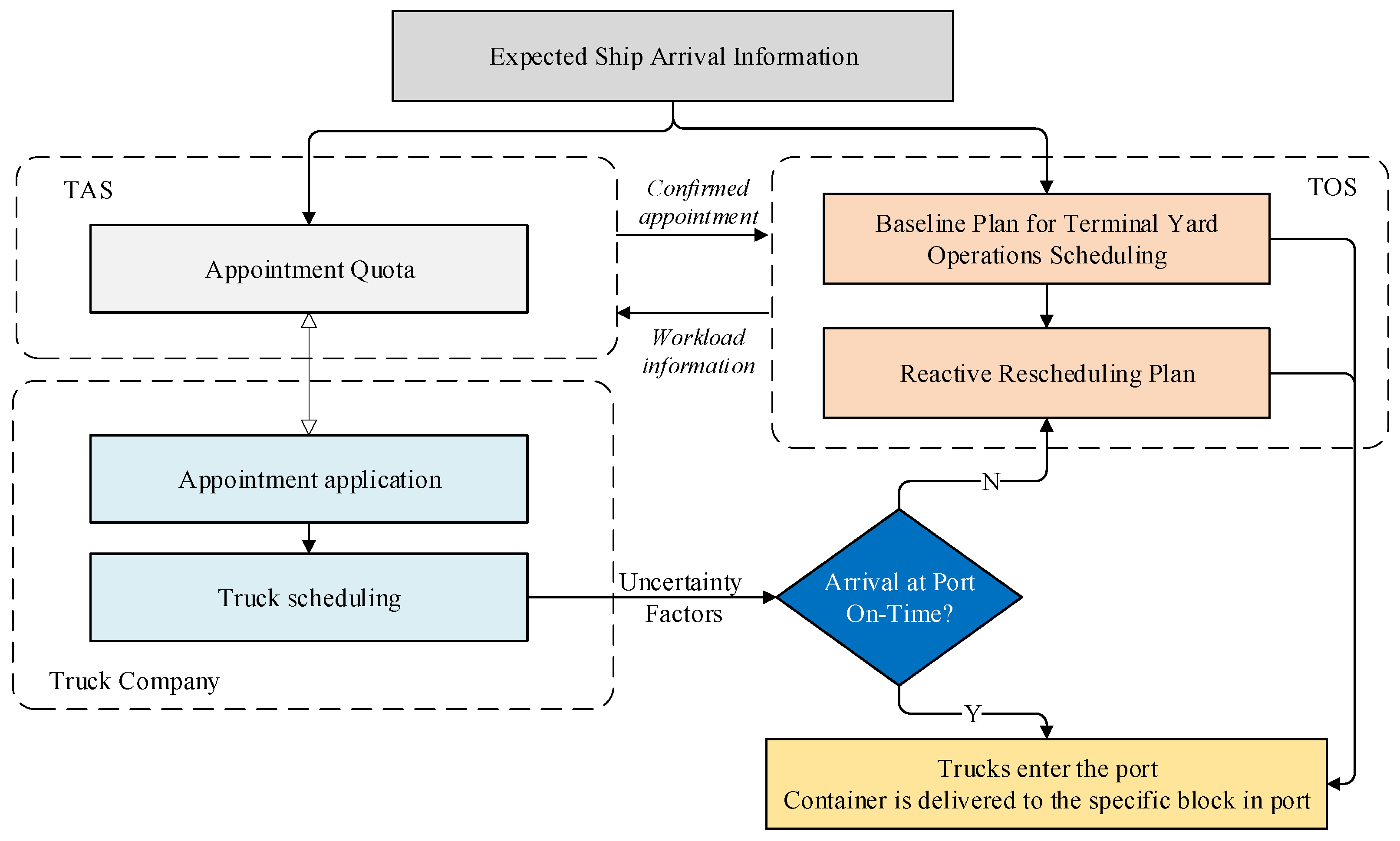
The data of truck arrivals, indexed by container identity (ID), are collected from the TOS. TOS refers to the software system used to manage and coordinate operations within a terminal. It handles tasks such as resource allocation, scheduling, and tracking of cargo, vehicles, and personnel to ensure efficient terminal operations. For each container, gate-in time, appointment start time, appointment end time, as well as delivery truck ID, etc., are recorded in the system. According to the above information, truck appointments, truck no-shows, and actual truck arrivals for each appointment period can be counted. In addition, this paper obtains relevant weather information and the traffic congestion coefficient for each appointment period drawn from a weather website and Baidu Maps’ big data platform, respectively.

To evaluate the model’s predictive performance and stability across different time scales, we first combined Data A and Data B to form a comprehensive dataset for model training. This unified training approach leverages the full range of information from both datasets, potentially enhancing the model’s ability to learn diverse patterns. After training the model on the combined dataset of Data A and Data B, we treated Data A and Data B separately for prediction. This approach allows us to assess whether the model can consistently perform well under varying temporal contexts and capture underlying patterns that may differ due to seasonal, operational, or external factors (e.g., weather, traffic). The separate treatment of Data A and Data B also allows us to explore whether there are significant differences in truck arrival patterns between the two periods, which could provide insights into the impact of temporal variations on prediction accuracy. For example, the weather conditions and traffic patterns in 2023 and 2024 may differ due to changes in port operations or external factors.

4.2.2. Outlier Detection and Missing Values Handling

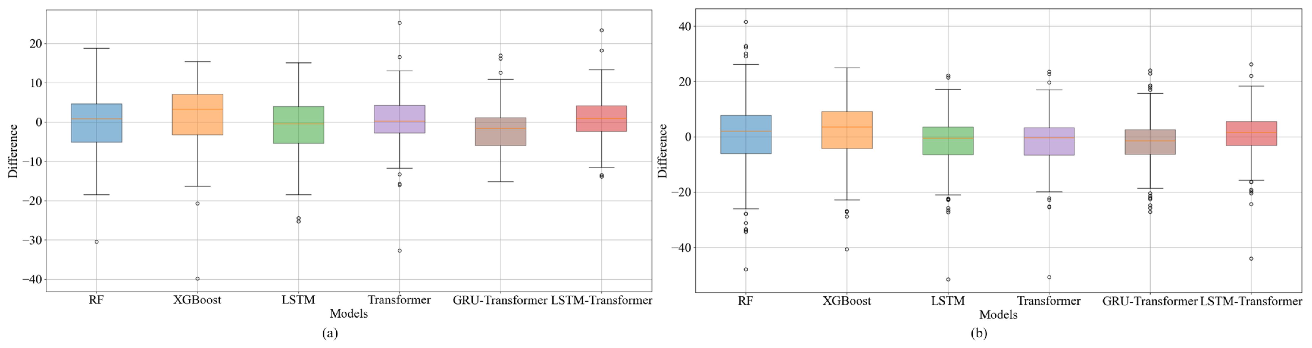
This paper employs the box plot method to detect outliers. The primary advantage of box plots is that they are resilient to outliers, enabling them to accurately and consistently represent the data’s distribution while aiding in data cleaning. For detected outliers, we treat them as missing values, as missing values can be imputed using information from existing variables. Rather than removing missing values, which would result in information loss, we use the KNN imputer for imputation, which calculates the values of k neighboring samples that are similar to the missing value sample to fill the missing values.

4.2.3. Data Processing

By collecting original data, we can find that the traffic congestion coefficient is a continuous variable greater than one, and we retain three decimals. The truck appointments, the truck no-shows, and the actual arrivals are integer variables greater than zero and do not need to be processed. Weather conditions typically encompass sunny, cloudy, rainy, foggy, and snowy days. Given that adverse weather conditions such as rain, fog, and snow significantly affect driving safety, these conditions are converted into binary variables, classified as “adverse” or “non-adverse”. There are 12 appointment periods in a day, and the appointment time period can be regarded as a multi-categorical variable, which is a discrete integer ranging from 1 to 12. If the discrete values are directly input, the model may mistakenly regard the relationship between these values as an ordered or linear relationship. Therefore, when building the model, we use the one-hot encoding technology to convert x₁ into 12 dummy variables. This approach can help the model better understand the categorical nature of this feature, avoid introducing wrong ordinal assumptions, and improve the accuracy of the model.

Table 1. Information on the datasets.

Factors	Variable Names	Variable Description	Data Sources
Weather conditions	Adverse weather	No = 0; Yes = 1	Weather website (https://tianqi.2345.com/, accessed on 1 July 2024.)
Appointment periods	Appointment periods	Convert to 12 dummy variables	TOS
Truck appointments	Truck appointments	Integer variable
Actual no-shows	Actual no-shows	Integer variable
Actual truck arrivals	Actual truck arrivals	Integer variable
Traffic conditions	Congestion coefficient	Continuous variable	Baidu Maps Traffic and Transportation Big Data Platform (https://jiaotong.baidu.com/, accessed on 1 July 2024)

illustrates the details of the datasets. These features are on vastly different scales, which complicates the training process of the model. To address this, this paper adopts data normalization. Normalization is a technique in deep learning that minimizes the likelihood of gradient explosions, accelerates convergence, stabilizes training, and boosts model performance [28]. Thus, before being input into algorithms, all raw data except binary variables and dummy variables are normalized using the following formula:

$$x^{\prime }={\displaystyle \frac{x-min(x)}{max(x)-min(x)}}$$

(20)

where the range of the normalized data are [0, 1], where $min(x)$ and $max(x)$ represent the minimum and maximum values of the sample data $x$, respectively.

Table 2. The statistics of datasets.

Factors	Data A				Data B
	Mean	Std	Skewness	Kurtosis	Mean	Std	Skewness	Kurtosis
x1	6.50	3.46	0.00	−1.22	6.50	3.45	0.00	−1.22
x2	0.09	0.28	2.98	6.89	0.05	0.23	3.91	13.32
x3	1.14	0.12	1.14	0.66	1.15	0.18	−0.21	−0.22
x4	28.26	26.38	0.96	0.41	43.33	33.06	0.64	−0.08
x5	1.05	1.84	2.61	8.15	1.03	1.83	3.44	19.99
x6	28.23	26.40	0.96	0.40	43.33	33.06	0.64	−0.08
x7	1.14	0.12	1.14	0.65	1.15	0.18	−0.21	−0.23
x8	28.17	26.83	1.04	0.60	43.32	32.52	0.71	0.01
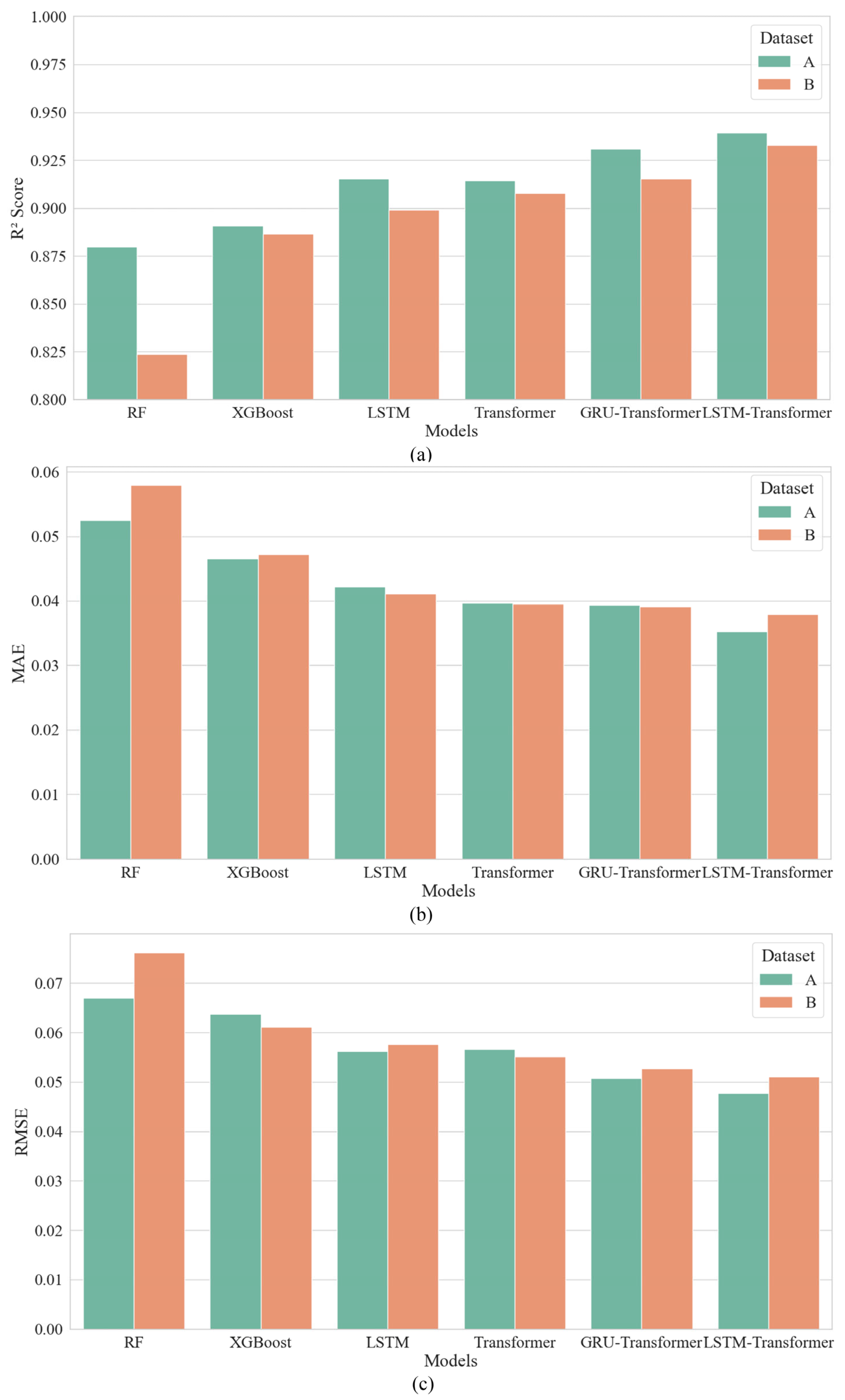
x9	28.24	26.80	1.03	0.60	43.33	32.51	0.72	0.01

presents the statistics of the two datasets. It can be seen that some factors of the two datasets have obvious differences in mean value, standard deviation (Std), skewness, and kurtosis. It indicates that there are differences in the centralized tendency, dispersion degree, and the sharpness of the two datasets. Training the LSTM-Transformer model on two datasets that have certain different statistical characteristics can significantly enhance the model’s performance and generalization capabilities. The training set comprises 80% of the two datasets, used for training model parameters. Then, 20% of each dataset is taken as the test set which is used for evaluating model performance.

4.3. Hyper-Parameter Tuning

To effectively train the model, it is essential to preset hyper-parameters that affect the learning process, such as the number of neurons, learning rate, and batch size. The learning efficiency and convergence of a model can vary based on hyper-parameter settings, and inappropriate hyper-parameters can lead to reduced performance. As there is no universally optimal value for hyper-parameters, it is necessary to find the best settings through hyper-parameter tuning. However, manually tuning hyper-parameters is both time-consuming and inefficient, and it is challenging to ensure that the optimal values are found. To address this challenge, we employ Optuna, an open-source hyper-parameter optimization framework grounded in Bayesian optimization algorithms. Optuna enables efficient and automatic hyper-parameter search by intelligently exploring the hyper-parameter space [29]. It supports multiple optimization algorithms, including tree-structured parzen estimator (TPE), and integrates seamlessly with leading machine learning libraries such as PyTorch 1.8.0, TensorFlow, Scikit-Learn, and XGBoost [25].

During the training phase, we employed mean square error (MSE) as the loss function and ADAM [30] as the optimizer. The hyper-parameter tuning process involved 100 trials, where each trial evaluated a unique combination of hyper-parameters. The model was trained for 100 epochs in each trial to refine predictions and better approximate actual values. Figure 5 illustrates the optimization process, with the x-axis representing the trial number (i.e., the number of evaluations of hyperparameter combinations) and the y-axis representing the model loss. This figure allows us to observe the changes in model performance throughout the optimization process, showing whether the objective value improves as the number of trials increases. The results demonstrate that Optuna effectively reduced the model loss, indicating successful optimization of the hyper-parameters.

Table 3. Results of model hyper-parameters tuning.

Hyper-Parameters	Meaning	Range of Tuning	Results
trans_nheads	The number of transformer heads	1~6	2
lstm_hidden_size	The dimension of the LSTM hidden layer	32~256	208
lstm_num_layers	The number of LSTM layers	1~3	2
trans_num_layers	The number of transformer layers	1~3	1
learning_rate	The learning rate for the optimizer	0.00001~0.1	0.00005

shows the hyper-parameters of the LSTM-Transformer model that we tuned using Optuna, the search range of hyper-parameters, and the best hyper-parameters determined by Optuna after 100 trials.

Figure 6 shows the interaction between hyper-parameters and the impact of different values on model performance, where the x-axis represents different hyper-parameters, with each vertical axis corresponding to a hyper-parameter, and the y-axis shows the value range of each hyper-parameter. Each line represents a trial, connecting the hyper-parameter values with the objective value. This figure helps analyze the relationship between hyper-parameter combinations and model performance, identifying which combinations lead to better optimization results.

4.4. Evaluation Metric

The coefficient of determination $R^2$, mean absolute error (MAE), and root mean square error (RMSE) are widely recognized metrics for model performance evaluating. The $R^2$ is used to measure the degree of fit between the predicted values and the actual values, with the closer the value is to one the better the fit. The MAE is a metric to measure the size of the prediction error with lower values indicating better performance. The RMSE is commonly used to address the discrepancies between estimates or predicted values and actual values in real settings. The smaller RMSE values indicate better outcomes and reflect the accuracy of models. The formulas for the coefficient of determination $R^2$, MAE, and RMSE are as follows:

$$R^2=1-{\displaystyle \frac{{\displaystyle \sum _{i=1}^n}{(y_i-\widehat{y_i})}^2}{{\displaystyle \sum _{i=1}^n}{(y_i-\overline{y})}^2}}$$

(21)

$$\mathrm{MAE}={\displaystyle \frac{{\displaystyle \sum _{i=1}^n}|y_i-\widehat{y_i}|}{n}}$$

(22)

$$\mathrm{RMSE}=\sqrt{{\displaystyle \frac{{\displaystyle \sum _{i=1}^n}{\left(y_i-\widehat{y_i}\right)}^2}{n}}}$$

(23)

where $y_i$ is actual value, $\widehat{y_i}$ is predicted value, $\overline{y}$ is mean of actual values, and $n$ is the number of samples.

5. Experiments and Analysis

5.1. Model Performance on One-Step Forecasting

Experiments were conducted on a PC running Windows with a 12th Gen Intel (R) Core (TM) i7-12700 2.10 GHz. Programming was conducted in Python 3.10, using the deep learning library Pytorch 1.8.0. To evaluate the performance of the LSTM-Transformer model, we first make one-step forecasting for actual truck arrivals on two datasets of different sample sizes.

Table 4. The performance of models on datasets.

Datasets	Model	R2	MAE	RMSE	Gap1 (%)	Gap2 (%)	Gap3 (%)
Data A	RF	0.8797	0.0525	0.0670	6.76	49.15	40.46
	XGBoost	0.8908	0.0465	0.0637	5.50	32.10	33.54
	LSTM	0.9152	0.0422	0.0562	2.73	19.89	17.82
	Transformer	0.9144	0.0397	0.0566	2.82	12.78	18.66
	GRU-Transformer	0.9309	0.0393	0.0508	0.94	11.65	6.50
	LSTM-Transformer	0.9392	0.0352	0.0477	-	-	-
Data B	RF	0.8238	0.0579	0.0761	12.38	52.77	48.92
	XGBoost	0.8864	0.0472	0.0611	5.26	24.54	19.57
	LSTM	0.8990	0.0411	0.0576	3.83	8.44	12.72
	Transformer	0.9077	0.0395	0.0551	2.84	4.22	7.83
	GRU-Transformer	0.9152	0.0391	0.0527	1.99	3.17	3.13
	LSTM-Transformer	0.9327	0.0379	0.0511	-	-	-

Note: $\mathrm{Gap}1={\displaystyle \frac{R^2(\mathrm{LSTM}\text{-}\mathrm{Transformer})-R^2(\mathrm{Baseline} \mathrm{model})}{R^2(\mathrm{Baseline} \mathrm{model})}}$, $\mathrm{Gap}2={\displaystyle \frac{\mathrm{MAE}(\mathrm{Baseline} \mathrm{model})-\mathrm{MAE}(\mathrm{LSTM}\text{-}\mathrm{Transformer})}{\mathrm{MAE}(\mathrm{LSTM}\text{-}\mathrm{Transformer})}}$, $\mathrm{Gap}3={\displaystyle \frac{\mathrm{RMSE}(\mathrm{Baseline} \mathrm{model})-\mathrm{RMSE}(\mathrm{LSTM}\text{-}\mathrm{Transformer})}{\mathrm{RMSE}(\mathrm{LSTM}\text{-}\mathrm{Transformer})}}$.

shows the results of the LSTM-Transformer model and baseline models, and Figure 7 shows visualized results.

Based on Data A and Data B, it presents an average improvement (Gap1, Gap2, and Gap3) of 3.75%, 25.11%, 23.40% and 5.26%, 18.63%, 18.43%, respectively, compared to the mean values of other models. LSTM-Transformer has achieved the best prediction results on both datasets, which demonstrates well the effectiveness and generalization ability of LSTM-Transformer. Moreover, we subtract the actual value from the predicted value, and draw the results into a box plot, as shown in Figure 8, where the x-axis is the different models and the y-axis is difference. The smaller the difference, the better the prediction performance. It can be seen that the predictions by LSTM-Transformer are the closest to the real data, indicating that LSTM-Transformer has the best prediction performance.

As can be seen from the table, the performance of the models on different datasets varies, because Data A and Data B differ in terms of sample size, temporal distribution, and operational complexity (e.g., variations in truck arrival, weather conditions, and traffic congestion), causing the differences in dataset length, distribution, and complexity between Data A and Data B, which can lead to variations in model performance. However, our experimental results demonstrate that the LSTM-Transformer model exhibits remarkable robustness across both datasets, with consistently high-performance metrics (R²: 0.9392 for Data A and 0.9327 for Data B; MAE: 0.0352 for Data A and 0.0379 for Data B; RMSE: 0.0477 for Data A and 0.0511 for Data B). This robustness can be attributed to the model’s ability to capture both long-term dependencies and complex temporal patterns through the integration of the LSTM and transformer architectures. In contrast, other models show more significant variations in performance between the two datasets. For example, the RF model’s R² decreases from 0.8797 (Data A) to 0.8238 (Data B), and the LSTM model’s R² declines from 0.9152 (Data A) to 0.8990 (Data B). This highlights the LSTM-Transformer model’s ability to generalize well across datasets with different characteristics and underscores the model’s potential as a reliable tool for predicting truck arrivals and optimizing terminal operations in diverse scenarios.

5.2. Model Performance on Multi-STEP Forecasting

As Figure 9 shows, when making two-step predictions, the average RMSE of all models increases significantly, but the average RMSE of transformer, GRU-Transformer and LSTM-Transformer are all low and close. Transformer and GRU-Transformer perform well in individual steps (such as steps 2 to 3), but as the number of prediction steps increases, all models except LSTM-Transformer show different degrees of error accumulation and fluctuation. In contrast, LSTM-Transformer, relying on the complementarity of LSTM’s ability to depict local temporal dependencies and transformer’s global attention mechanism, continues to maintain a lower average RMSE in medium- and long-term predictions (steps 4 to 7), which is significantly different from other models. This shows that LSTM-Transformer is more robust and generalizable in modeling long sequence dynamics and can effectively alleviate the error accumulation problem in multi-step prediction scenarios, thereby showing better performance in long-term prediction tasks.

5.3. Features Grouping

To better study the impact of features on the actual truck arrival, we conducted a Pearson correlation analysis between each feature and the actual truck arrival based on Data A, as Figure 10 shows.

To focus on the most significant features influencing actual truck arrivals, we selected features with a Pearson correlation coefficient greater than 0.4, a threshold that indicates a moderate to strong positive correlation [31]. This ensures that we are capturing the impact of key features on model performance while reducing noise from weakly correlated or irrelevant features. To further validate the model’s performance and explore potential feature interactions, we constructed six feature groups by progressively adding features based on their Pearson correlation coefficients. The feature groups are defined as follows: top one feature (1F), top two features (2F), top three features (3F), top four features (4F), top five features (5F), and all features (AF). This approach allows us to systematically evaluate the model’s performance and robustness under different feature combinations and investigate whether there are synergistic interactions between features.

Table 5. The best hyper-parameters of different feature groups.

Feature Groups	Features	Hyper-Parameters
		Trans_Nheads	Hidden_Size	Lstm_Num_Layers	Trans_Num_Layers	Learning_Rate
1F	x4	1	103	2	1	0.00002
2F	x4, x9	3	183	2	2	0.00002
3F	x4, x9, x6	4	172	2	1	0.00004
4F	x4, x9, x6, x8	2	222	2	1	0.00019
5F	x4, x9, x6, x8, x5	2	112	1	1	0.00030
AF	All Features	2	208	2	1	0.00005

summarizes the best hyper-parameters of different feature groups.

5.4. Feature Groups Comparisons and Analysis

In order to validate the accuracy of the proposed LSTM-Transformer model, we selected RF, XGBoost, LSTM, GRU-Transformer, and transformer models for comparison. For these models, the hyper-parameters were optimized by Optuna, manual parameter adjustment, or grid search to ensure the validity of the experimental results. All models were trained on the same training set and predicted on the test set of Data A based on different feature combinations. The performance of different models in forecasting the actual truck arrivals was assessed using the test set, and the results are visualized, as shown in Figure 11. The details of the model performance evaluation metrics of each model considering different feature groups are shown in Appendix A. Moreover, in order to compare the prediction performance of different models considering different feature groups, a box plot of the residuals is drawn, as shown in Figure 12.

Based on the results, the following conclusions can be drawn:

(1)

Compared to other popular machine learning models, the LSTM-Transformer model demonstrates superior and more stable performance across all feature groups, consistently achieving high prediction accuracy with minimal variation in results and maintaining lower MAE and RMSE values, excelling in capturing both short-term temporal dependencies and long-range patterns by integrating the strengths of LSTM and transformer. Although its prediction accuracy for certain feature groups, such as 1F (x₄) and 3F (x₄, x₆, x₉), is marginally lower than that of the standalone LSTM or transformer models due to the added complexity of the LSTM-Transformer architecture in scenarios where simpler models suffice—such as the 1F feature group, where the standalone LSTM effectively models short-term dynamics, and the 3F feature group, where the inclusion of x₆ may introduce redundant temporal information—these differences are not statistically significant, underscoring the LSTM-Transformer model’s robust predictive capabilities and suitability for complex forecasting tasks in container terminal applications.

(2)

The results show that as the number of features increases, the prediction performance of GRU-Transformer and LSTM-Transformer is gradually improving overall. However, LSTM-Transformer performs better, with the best performance under feature group AF. This suggests that the features in our study have complementary effects. Even though factors such as weather, congestion coefficient, and appointment periods may be weakly correlated with the actual truck arrivals, the LSTM-Transformer model can still extract more information from these factors that are closely related to the truck no-shows. The combination of features enables the model to capture more complex patterns in the data, helping to improve the model’s prediction accuracy.

(3)

Although LSTM and transformer exhibit high prediction accuracy, significantly outperforming RF and XGBoost, their accuracy tends to decrease as the number of feature variables increases, with LSTM showing a decline and transformer experiencing fluctuating decreases. This is primarily because when there are too many features relative to the number of samples, both the LSTM and transformer models exhibit unstable learning and are prone to overfitting. Although GRU-Transformer has a higher prediction accuracy than transformer, the accuracy and overall performance are still lower than LSTM-Transformer. The LSTM-Transformer model proposed in this paper, by integrating the temporal data processing capabilities of LSTM with the efficient context capturing features of the transformer, effectively avoids overfitting issues and enhances the model’s generalization capabilities in multi-feature environments. Additionally, the transformer component, through its self-attention mechanism, focuses on the features most relevant to the prediction task, thereby filtering out unnecessary noise.

5.5. Sensitivity Analysis of Input Features

To further determine the influence of different features, the input is decomposed and analyzed. In detail, in this section we investigate the extent to which the truck appointment information, truck no-show, actual truck arrivals in other appointment periods, and the features (appointment period, weather condition, traffic congestion coefficient) with lower Pearson correlation coefficients affect the prediction accuracy. The following nine types of experiments with different input features are therefore set up. Their results are compared with the control group.

Test 1: LSTM-Transformer is fed with the dataset without the truck appointment information ($x_4$, $x_6$).

Test 2: LSTM-Transformer is fed with the dataset without the truck no-show information ($x_5$).

Test 3: LSTM-Transformer is fed with the dataset without actual truck arrivals in the previous two appointment periods ($x_8$, $x_9$).

Test 4: LSTM-Transformer is fed with the dataset without $x_4$, $x_5$, $x_6$, $x_8$, and $x_9$.

Test 5: LSTM-Transformer is fed with the dataset without the appointment period ($x_1$).

Test 6: LSTM-Transformer is fed with the dataset without the weather conditions ($x_2$).

Test 7: LSTM-Transformer is fed with the dataset without the traffic congestion coefficient ($x_3$, $x_7$).

Test 8: LSTM-Transformer is fed with the dataset without $x_1$, $x_2$, $x_3$, and $x_7$.

Control group: LSTM-Transformer is fed with all the input datasets.

Table 6. The comparison results with different input features.

	R2	MAE	RMSE
Test 1	0.5860	0.0915	0.1243
Test 2	0.9112	0.0452	0.0576
Test 3	0.9260	0.0407	0.0526
Test 4	0.3471	0.1156	0.1561
Test 5	0.9352	0.0349	0.0491
Test 6	0.9374	0.0357	0.0483
Test 7	0.9194	0.0427	0.0548
Test 8	0.9315	0.0353	0.0506
Control group	0.9392	0.0352	0.0477

shows the comparison results with different input features. Firstly, Test 1 shows significant difference from the control group, indicating that truck appointment information is an important factor affecting truck arrivals and is crucial for accurately predicting actual truck arrivals. During the implementation of the TAS, trucks can enter the port smoothly only when they arrive at the port within the appointment period. Late arrivals require rescheduling, which can incur additional costs. Therefore, except for force majeure, most trucks strive to ensure they arrive as scheduled, making the truck appointments of the appointment period an important basis for predicting actual truck arrivals. Secondly, the results of Test 2 and Test 3 suggest that information about the previous appointment periods’ truck no-shows and actual truck arrivals helps improve prediction accuracy. This is mainly because trucks that arrive late and miss their appointments often reschedule for subsequent periods, leading to actual arrivals in later periods that are higher than the scheduled volumes. Finally, the comparison of Test 4 and the control group once again demonstrates the importance of truck appointment information, previous appointment periods’ truck no-show information, and actual truck arrival information.

Test 5–8 shows that although the Pearson correlation coefficients of the weather, traffic congestion coefficient, and appointment period are relatively low at the overall data level, including these features can effectively improve the model prediction accuracy. Different appointment periods often correspond to different peak or idle periods, and the Pearson correlation coefficient may underestimate the actual impact of a specific period after averaging the overall data. Extreme weather and severe congestion often occur locally or in a small number of appointment periods, significantly disrupting arrival behavior. Therefore, the correlation coefficient cannot fully capture their impact, and they often have a key impact locally, or an interaction with other features, which can effectively improve the model’s prediction accuracy for complex real-life situations.

It is noteworthy that the control group performed the best, with the smallest difference from the actual values, indicating that the LSTM-Transformer model can effectively utilize various features to capture more information and identify hidden relationships between these features to enhance prediction accuracy, further validating the effectiveness of the LSTM-Transformer model.

6. Conclusions

This paper introduces improvements to the transformer deep learning model by designing a model structure that addresses both long-term and short-term trends, effectively capturing historical trends for prediction, improving the prediction accuracy of the actual truck arrivals. In comparative assessments, the LSTM-Transformer model outperforms other machine learning models, showing robust predictive performance and excellent generalization ability on datasets. This validates the improved transformer-based model proposed in this paper, showing its ability to accurately predict the actual truck arrivals and how, significantly, it can play an important role in the actual production activities of container terminals. This paper also discusses the impact of various factors on the actual arrival of container trucks, proving that the truck appointment information, truck no-show information, actual truck arrivals in previous two appointment periods, weather, and traffic will have an impact on the actual truck arrivals, providing a reference for future planning of terminal yard operations. The selected features are widely applicable to ports with TAS, thus the model established in this paper is also applicable to other ports with TAS. However, when the data characteristics of a port differ significantly from those in this paper, it is necessary to retrain the model using that port’s dataset. For ports without TAS, certain features may not be available. In such cases, we propose leveraging historical data and alternative features, such as the time series of daily truck arrivals, weekday parameters, and vessel-related variables, ensuring the model’s adaptability to ports with different operational characteristics.

However, this paper still has some limitations. In the future, we plan to introduce advanced techniques to analyze the weights of feature variables and refine the model’s algorithms, enabling a clearer identification of the most impactful factors. To further improve the model, we will explore a hybrid architecture that combines the predictive power of deep learning with the interpretability of traditional machine learning methods. This will be complemented by detailed case studies to analyze the impact of specific features in real-world scenarios, providing deeper insights into the relationships between features and predictions. While our model demonstrates strong performance for the port being studied, its generalizability to other ports with different operational constraints remains limited. To address this, we will collect data from multiple ports, incorporate port-specific features, and leverage transfer learning techniques to enhance adaptability. Moreover, we will investigate additional methodologies, such as data augmentation, synthetic data generation, and real-time adaptation techniques, to address data scarcity and dynamic operational changes. Integrating external data sources, such as real-time traffic, port operations, and socioeconomic factors, will also be explored to provide a richer context and further improve the prediction accuracy. As research on influential factors advances and the scope of data collection expands, the accuracy of truck arrival predictions using deep learning techniques will continue to improve, paving the way for more robust and practical applications.

References

1. Giuliano, G.; O’Brien, T. Reducing Port-Related Truck Emissions: The Terminal Gate Appointment System at the Ports of Los Angeles and Long Beach. Transp. Res. Part Transp. Environ. 2007, 12, 460–473. [Google Scholar] [CrossRef]
2. Ma, M.; Fan, H.; Ji, M.; Guo, Z. Integrated optimization of truck appointment for export containers and crane deployment in a container terminal. J. Transp. Syst. Eng. Inf. Technol. 2018, 18, 202–209. [Google Scholar] [CrossRef]
3. Li, N.; Chen, G.; Ng, M.; Talley, W.K.; Jin, Z. Optimized Appointment Scheduling for Export Container Deliveries at Marine Terminals. Marit. Policy Manag. 2020, 47, 456–478. [Google Scholar] [CrossRef]
4. Fan, H.; Peng, W.; Ma, M.; Yue, L. Storage Space Allocation and Twin Automated Stacking Cranes Scheduling in Automated Container Terminals. IEEE Trans. Intell. Transp. Syst. 2022, 23, 14336–14348. [Google Scholar] [CrossRef]
5. Zhao, W.; Goodchild, A.V. Using the Truck Appointment System to Improve Yard Efficiency in Container Terminals. Marit. Econ. Logist. 2013, 15, 101–119. [Google Scholar] [CrossRef]
6. Zeng, Q.; Feng, Y.; Yang, Z. Integrated Optimization of Pickup Sequence and Container Rehandling Based on Partial Truck Arrival Information. Comput. Ind. Eng. 2019, 127, 366–382. [Google Scholar] [CrossRef]
7. Cai, L.; Li, W.; Zhou, B.; Li, H.; Yang, Z. Robust Multi-Equipment Scheduling for U-Shaped Container Terminals Concerning Double-Cycling Mode and Uncertain Operation Time with Cascade Effects. Transp. Res. Part C Emerg. Technol. 2024, 158, 104447. [Google Scholar] [CrossRef]
8. Yang, Z.; Chen, G.; Moodie, D.R. Modeling Road Traffic Demand of Container Consolidation in a Chinese Port Terminal. J. Transp. Eng. 2010, 136, 881–886. [Google Scholar] [CrossRef]
9. Ma, M.; Zhao, W.; Fan, H.; Gong, Y. Collaborative Optimization of Yard Crane Deployment and Inbound Truck Arrivals with Vessel-Dependent Time Windows. J. Mar. Sci. Eng. 2022, 10, 1650. [Google Scholar] [CrossRef]
10. Huang, Y.; Shen, L.; Liu, H. Grey Relational Analysis, Principal Component Analysis and Forecasting of Carbon Emissions Based on Long Short-Term Memory in China. J. Clean. Prod. 2019, 209, 415–423. [Google Scholar] [CrossRef]
11. Zhou, H.; Zhang, S.; Peng, J.; Zhang, S.; Li, J.; Xiong, H.; Zhang, W. Informer: Beyond Efficient Transformer for Long Sequence Time-Series Forecasting. Proc. AAAI Conf. Artif. Intell. 2021, 35, 11106–11115. [Google Scholar] [CrossRef]
12. Vaswani, A.; Shazeer, N.; Parmar, N.; Uszkoreit, J.; Jones, L.; Gomez, A.N.; Kaiser, Ł.; Polosukhin, I. Attention is all you need. Adv. Neural Inf. Process. Syst. 2017, 30, 1–11. [Google Scholar]
13. Guo, Y.; Mao, Z. Long-Term Prediction Model for NOx Emission Based on LSTM–Transformer. Electronics 2023, 12, 3929. [Google Scholar] [CrossRef]
14. Yan, H.; Deng, B.; Li, X.; Qiu, X. TENER: Adapting Transformer Encoder for Named Entity Recognition. arXiv 2019, arXiv:1911.04474. [Google Scholar]
15. Farhan, J.; Ong, G.P. Forecasting Seasonal Container Throughput at International Ports Using SARIMA Models. Marit. Econ. Logist. 2018, 20, 131–148. [Google Scholar] [CrossRef]
16. Yi, Y.; Seyed Sadr, S.T. Algorithm Design of Port Cargo Throughput Forecast Based on the ES-Markov Model. Discret. Dyn. Nat. Soc. 2022, 2022, 7029980. [Google Scholar] [CrossRef]
17. Mateo-Pérez, V.; Corral-Bobadilla, M.; Ortega-Fernández, F.; Rodríguez-Montequín, V. Determination of Water Depth in Ports Using Satellite Data Based on Machine Learning Algorithms. Energies 2021, 14, 2486. [Google Scholar] [CrossRef]
18. Peng, W.; Bai, X.; Yang, D.; Yuen, K.F.; Wu, J. A Deep Learning Approach for Port Congestion Estimation and Prediction. Marit. Policy Manag. 2023, 50, 835–860. [Google Scholar] [CrossRef]
19. Yoo, S.-L.; Kim, K.-I. Deep Learning-Based Prediction of Ship Transit Time. Ocean Eng. 2023, 280, 114592. [Google Scholar] [CrossRef]
20. Li, N.; Sheng, H.; Wang, P.; Jia, Y.; Yang, Z.; Jin, Z. Modeling Categorized Truck Arrivals at Ports: Big Data for Traffic Prediction. IEEE Trans. Intell. Transp. Syst. 2023, 24, 2772–2788. [Google Scholar] [CrossRef]
21. Breiman, L. Random Forests. Mach. Learn. 2001, 45, 5–32. [Google Scholar] [CrossRef]
22. Chen, T.; Guestrin, C. XGBoost: A Scalable Tree Boosting System. In Proceedings of the 22nd ACM SIGKDD International Conference on Knowledge Discovery and Data Mining, San Francisco, CA, USA, 13–17 August 2016; ACM: New York, NY, USA, 2016; pp. 785–794. [Google Scholar]
23. Somu, N.; M R, G.R.; Ramamritham, K. A Hybrid Model for Building Energy Consumption Forecasting Using Long Short Term Memory Networks. Appl. Energy 2020, 261, 114131. [Google Scholar] [CrossRef]
24. Sun, K.; Qaisar, I.; Khan, M.A.; Xing, T.; Zhao, Q. Building Occupancy Number Prediction: A Transformer Approach. Build. Environ. 2023, 244, 110807. [Google Scholar] [CrossRef]
25. Ahn, J.M.; Kim, J.; Kim, H.; Kim, K. Harmful Cyanobacterial Blooms Forecasting Based on Improved CNN-Transformer and Temporal Fusion Transformer. Environ. Technol. Innov. 2023, 32, 103314. [Google Scholar] [CrossRef]
26. He, K.; Zhang, X.; Ren, S.; Sun, J. Deep Residual Learning for Image Recognition. In Proceedings of the 2016 IEEE Conference on Computer Vision and Pattern Recognition (CVPR), Las Vegas, NV, USA, 27–30 June 2016; pp. 770–778. [Google Scholar]
27. Ba, J.L.; Kiros, J.R.; Hinton, G.E. Layer Normalization. arXiv 2016, arXiv:1607.06450. [Google Scholar]
28. Xing, T.; Sun, K.; Zhao, Q. MITP-Net: A Deep-Learning Framework for Short-Term Indoor Temperature Predictions in Multi-Zone Buildings. Build. Environ. 2023, 239, 110388. [Google Scholar] [CrossRef]
29. Akiba, T.; Sano, S.; Yanase, T.; Ohta, T.; Koyama, M. Optuna: A Next-Generation Hyperparameter Optimization Framework. In Proceedings of the 25th ACM SIGKDD International Conference on Knowledge Discovery & Data Mining, Anchorage, AK, USA, 4–8 August 2019; ACM: New York, NY, USA, 2019; pp. 2623–2631. [Google Scholar]
30. Kingma, D.P.; Ba, J. Adam: A Method for Stochastic Optimization. arXiv 2014, arXiv:1412.6980. [Google Scholar]
31. Benesty, J.; Chen, J.; Huang, Y.; Cohen, I. Pearson Correlation Coefficient. In Noise Reduction in Speech Processing; Springer Topics in Signal Processing; Springer: Berlin/Heidelberg, Germany, 2009; Volume 2, pp. 1–4. ISBN 978-3-642-00295-3. [Google Scholar]
Figure 1. Schematic diagram.
Jmse 13 00405 g001
Figure 2. LSTM network.
Jmse 13 00405 g002
Figure 3. The structure of the self-attention mechanism.
Jmse 13 00405 g003
Figure 4. The structure of the LSTM-Transformer Model.
Jmse 13 00405 g004
Figure 5. Optimization progress visualization over trials.
Jmse 13 00405 g005
Figure 6. Parallel coordinate visualization of hyper-parameters.
Jmse 13 00405 g006
Figure 7. The visualization of model performance results. (a) R2, (b) MAE, and (c) RMSE.
Jmse 13 00405 g007
Figure 8. The difference between the actual value and the predicted value of each model on datasets. (a) Data A. (b) Data B.
Jmse 13 00405 g008
Figure 9. The multi-step prediction for models.
Jmse 13 00405 g009
Figure 10. The Pearson correlation coefficient between actual truck arrivals and different features.
Jmse 13 00405 g010
Figure 11. The performance evaluation results of different models considering different feature groups. (a) R2, (b) MAE, and (c) RMSE.
Jmse 13 00405 g011
Figure 12. The box plot of the residuals of different models considering different feature groups. (a) Feature group 1F. (b) Feature group 2F. (c) Feature group 3F. (d) Feature group 4F. (e) Feature group 5F. (f) Feature group AF.
Jmse 13 00405 g012