Research on Ellipse-Based Transient Impact Source Localization Methodology for Ship Cabin Structure

Abstract

This study explores the application of three localization methods in identifying transient impact sources in the ship cabin structure. These methods examined are based on energy curvature and cumulative error, time-reversed virtual focusing triangulation, and energy correlation localization. It presents an elliptical region-based transient impact source localization technique for the ship cabin structure. The center of the elliptical region is determined by calculating the arithmetic mean of the position coordinates obtained from three methods, and the long and short semi-axes of the ellipse are defined as three times the standard deviations in the horizontal and vertical directions, respectively, to construct an elliptical localization area for precise positioning. Experimental results indicate that the average error distance of this impact localization technique is 0.10 m, with the predicted position error of 22 impact points being 0 m. Among 15 impact points, 14 impact points have error distances ranging from 0 m to 0.40 m, while 1 impact point has an error distance of 1.08 m, primarily due to the weak connection between sensors and the ship cabin structure. The overall localization error of the ship cabin structure is low, meeting the required localization accuracy.

1. Introduction

Ship structures serving long-term in harsh environments such as the ocean are susceptible to the interaction of various loads. Sudden failures (such as the loosening of structural components) or low-speed impacts from foreign objects can induce damage in the structure, posing a significant threat to its reliability. Therefore, it is necessary to employ various acoustic and vibration sensors for health monitoring and localization of impact sources in the structure, thereby rapidly identifying the locations of abnormal impact sources and enhancing the quality maintenance level of ship structures [1,2,3,4].

Currently, commonly used methods for low-speed impact localization in structures based on vibration accelerometers are signal processing-based localization methods. These methods primarily involve arranging accelerometers on the structure to receive impact response signals and combining modern signal processing techniques with specific algorithms to achieve impact localization [5,6]. Researchers both domestically and internationally have proposed a multitude of structural impact localization methods, including hyperbolic localization [7,8], triangulation [9,10], four-point arc method [11,12], time-reversal focusing [13,14], and error function method [15,16,17,18,19]. The first three methods utilize the geometric relationship between wave arrival time, wave velocity, and sensor positions to achieve impact localization. Among them, the hyperbolic localization method calculates the focal distance by estimating the time difference of wave arrival at different sensors, thereby plotting two sets of hyperbolas and determining the intersection point as the impact source location [20,21]. The triangulation and four-point arc methods mainly extract the signal arrival time and establish a set of nonlinear equations based on the geometric relationship between sensors and the impact position, ultimately solving for the corresponding location results [22,23,24,25]. The general approach of these geometric localization methods is to first calculate the time difference of sensors and then use the wave velocity value within the structural region as a constant to solve the equation set, with the solution serving as the localization position. These methods, when applied to small-scale isotropic structures, yield relatively small error results. However, for large-scale complex anisotropic structures, the wave velocity is typically not constant, and using these methods for impact source localization can easily lead to larger errors. The time-reversal focusing method is a signal-processing technique based on wave theory. Its fundamental concept is that when the excitation signal propagates through the structural medium, it is affected by the medium’s inhomogeneity, resulting in scattering and attenuation. However, when these scattered signals propagate again in a direction opposite to the original path, they focus at the signal source location, forming a high-resolution focal point. The localization of structural impact sources can be achieved by measuring and analyzing the signal characteristics of this focal point [26,27]. The time-reversal focusing method can more accurately extract arrival times through signal enhancement. Wu, Z. [28] constructed a virtual time-reversal imaging function with impact position coordinates and narrowband group velocity as variables. By obtaining the adaptive time-reversal focusing image based on the maximum pixel curve corresponding to different group velocities, impact localization is realized. However, the accuracy of impact localization for large-scale complex anisotropic structures requires further investigation. The error function method is an emerging impact localization technique that acquires sensor arrival times to construct an error index function, achieving impact probability imaging localization based on the error index at each point within the structure, thereby avoiding the need to solve for wave velocity. Gorgin, R. [15] proposed a probability-based impact localization method for plate structures, introducing the root mean square threshold of the Time of Arrival (TOA) of impact waves to establish the localization equation of the error index, and validated the effectiveness of this localization method through experiments of steel ball impact on carbon fiber composite plates. Peng, T. [16] applied an error index-based collision localization algorithm in plate-shell and cylindrical-shell structures using the total residual error of the signal as the arrival time to construct the probability function of the collision point and verified the accuracy of the localization method under three different noise conditions. Yang, L. [17] proposed a new structural impact localization method that utilizes the complex Morlet wavelet transform to extract narrowband signals from the signal and calculate their modulus. An error function based on wave arrival time differences was constructed by measuring the arrival times and calculating the time differences between sensors. The method was validated on aluminum plates and composite-reinforced plates, demonstrating high localization accuracy. Shi, C. [18] proposed a new method for composite material impact localization, utilizing a piezoelectric sensor network to capture impact responses and extracting signal features through complex Morlet wavelet transform. Subsequently, the impact location is determined by constructing an error function and calculating the impact probability at each point within the structure. Impact experiments conducted on glass fiber-reinforced resin-based composite plates verified the effectiveness of this localization method. Yang, L. [19] introduced an error function probability imaging impact localization method, which extracts narrowband signals using complex Morlet wavelet transform and constructs an error function based on the time difference of arrival to calculate the probability value of the impact source. Drop hammer impact experiments on carbon fiber-reinforced composite-stiffened plates confirmed the effectiveness and accuracy of the impact method. The aforementioned error function-based localization methods do not rely on prior information such as wave velocity and are applicable for impact source localization in both anisotropic and isotropic structures. In addition to the aforementioned impact localization methods, data-driven structural impact localization methods have also been further studied in recent years. However, these methods require a large amount of data signals to pre-train the model before localization.

Current research on impact localization techniques has made certain advancements, particularly in the study of individual methods for specific applications. However, while numerous studies have focused on the impact localization performance of a single method, research on the integrated application of multiple localization methods in actual structures is relatively scarce. This research gap limits the comprehensive understanding of impact localization issues in complex structures, especially in environments with complex geometries and dynamic characteristics, such as ship cabin structures. This manuscript presents an impact localization experiment for transient impacts in ship cabin structures. In the experiment, the authors employed three different novel localization methods: the method based on energy curvature and cumulative error [29], the triangulation method based on time-reversed virtual focusing [30], and the method based on energy correlation [31]. Each of these methods has its unique advantages and limitations, but in practical applications, a single method often fails to meet the requirements of high precision and high reliability. To overcome this challenge, this manuscript proposes an elliptical region-based transient impact source localization technique for the ship cabin structure. The core of this technique lies in integrating the results of different localization methods, enhancing the accuracy and reliability of localization through comprehensive analysis and decision-making applications.

2. Localization Methods

The study applies a comprehensive localization analysis of transient impact sources in the ship cabin structure using three methods: localization based on energy curvature and cumulative error, triangulation based on time-reversed virtual focusing, and localization based on energy correlation. The method based on energy curvature and cumulative error determines the arrival times between different sensors by iteratively calculating the signal’s energy curvature until a non-zero value appears, then establishes an error function to solve for the minimum cumulative error to predict the impact location. The triangulation method based on time-reversed virtual focusing does not require constructing models or experimental means to determine the wave transfer function; it only focuses on the wave propagation velocity, and by obtaining the wave speed information, it can achieve the synthetic time-reversed focusing of Lamb waves in the structure. The localization method based on energy correlation theoretically establishes the relationship between sensor energy and the relative positions of sensors and the impact source, thereby directly achieving impact localization in the structure. The scene diagram of the impact positioning action is shown in Figure 1.

2.1. Localization Method Based on Energy Curvature and Cumulative Error

The principle of the impact localization method based on energy curvature and error function is to iteratively calculate the cumulative energy and curvature energy of signals from each sensor at different time points. The first non-zero moment of the signal curvature energy curve is taken as the predicted TOA. Based on the predicted TOA, a structural grid region is established, and an error function including the impact occurrence time is introduced for each pair of sensors. By minimizing the curvature cumulative energy error, the impact occurrence time is determined, thereby calculating the impact probability at each point in the structure. The grid with the highest impact probability is considered the predicted impact location [29]. The specific implementation process of this method is as follows:

(1)

The vibration signal a_i(t) collected by the acceleration sensor is zero-averaged, and the zero-averaged signal b_i(t) is obtained.

$$b_i(t)=a_i(t)-{\displaystyle \frac{{\displaystyle \sum _{n=1}^N{a}_i(n/f_s)}}{N}}$$

(1)

(2)

The maximum value of the absolute amplitude of the signal b_i(t) after zero-averaging is normalized, the normalized signal s_i(t) can be calculated, and the range of the s_i(t) value is between −1 and 1.

$$s_i(t)={\displaystyle \frac{b_i(t)}{\max \left|b_i\right|}}$$

(2)

(3)

For the preprocessed signal s_i(t), the acceleration sum of squares of the signal is calculated cumulatively, and the initial energy $E_{i,0}\left(t\right)$ can be obtained.

$$E_{i,0}\left(t\right)={\displaystyle \sum _{\tau =0}^t{s}_i{\left(\tau \right)}^2}$$

(3)

(4)

Solve the first-order derivative of the accumulated energy $E_{i,0}\left(t\right)$ twice consecutively to obtain the initial energy curvature $Q_{i,1}\left(t\right)$.

$$E_{i,1}\left(t\right)={\displaystyle \sum _{\tau =0}^t{Q}_{i,1}{\left(\tau \right)}^2}$$

(4)

(5)

Repeat the process from steps 3 to 4 four more times to obtain, respectively, the energy $E_{i,1}\left(t\right)$ and the energy curvature $Q_{i,2}\left(t\right)$ for the first cycle; the energy $E_{i,2}\left(t\right)$ and the energy curvature $Q_{i,3}\left(t\right)$ for the second cycle; the energy $E_{i,3}\left(t\right)$ and the energy curvature $Q_{i,4}\left(t\right)$ for the third cycle; and the final energy $E_{i,4}\left(t\right)$ after the fourth cycle.

(6)

The moment corresponding to the first non-zero value of $E_{i,4}\left(t\right)$ is taken as the TOA of each sensor.

(7)

Divide the structural impact monitoring area into several grids and find the distance Li between each grid point and each sensor.

(8)

Construct the cumulative error function formula as shown in Equation (5), then define the cumulative error value corresponding to any grid point at a certain value of time t_k in the time interval where the impact may occur, as follows:

$${\epsilon }_k\left(x_i,y_i\right)={\displaystyle \sum _{m=1}^N{\displaystyle \sum _{n=1}^N\left|\frac{TO{A}_m-t_k}{TO{A}_n-t_k}-\frac{\sqrt{{\left(x_i-x_m\right)}^2+{\left(y_i-y_m\right)}^2}}{\sqrt{{\left(x_i-x_n\right)}^2+{\left(y_i-y_n\right)}^2}}\right|}}$$

(5)

where N is the number of accelerometers, and (x_i, y_i) are the grid coordinates of the monitoring area. (x_m, y_m), (x_n, y_n) are the positional coordinates of sensors, and t_k is the computed time of impact occurrence.

(9)

Compare the cumulative error values at each sampling time t_k in the possible time interval, and take the position (x_i, y_i) corresponding to the minimum cumulative error as the localization result and the time t_k corresponding to the minimum cumulative error as the shock moment.

(10)

Define the impact probability of each grid point in the monitoring area, as shown in Equation (6), and take the grid position with the largest probability as the predicted impact coordinates, as shown in Figure 2.

$$PIL={\displaystyle \frac{\min ({\epsilon }_k(x_i,y_i))}{{\epsilon }_k(x_i,y_i)}}\times 100\%$$

(6)

2.2. Triangular Localization Method Based on Time-Reversal Virtual Focusing

The principle of the triangulation method based on time-reversed virtual focusing is to capture impact response signals using a sensor network and then reverse the signals in time, causing them to propagate backward along their original paths and focus at the impact source location [30]. Specifically, when a structure is impacted, the resulting stress waves are captured by sensors arranged on the structure. After undergoing time-reversal processing, these signals are re-emitted, and they return along their propagation paths, achieving energy concentration at the impact source [32]. The specific implementation process of this method is as follows:

(1)

Calculation of sensor vibration signal energy power: data inputs are selected from sensors with higher rankings in energy power.

(2)

Signal wavelet packet decomposition: Lamb waves are generated in the structure under excitation. The dispersive characteristics of Lamb waves result in a rich spectrum of frequency components within the original vibration signal, leading to significant frequency dispersion influence. Wavelet packet decomposition of signals is a time-frequency analysis technique that overcomes the frequency resolution limitations of traditional short-time Fourier transforms, providing localized time-frequency features of signals. Initially, a mother wavelet function that meets specific conditions is determined. Subsequently, the mother wavelet is scaled, translated, and convolved with the original signal to achieve decomposition at different scales and positions. Further, by recursively applying wavelet packet decomposition to both the high-frequency and low-frequency components of the signal, multi-level decomposition is realized to enhance frequency resolution. During the decomposition process, the signal is divided into approximation and detail components, forming a tree-like structure. Based on the analysis results, the signal is synthesized stepwise from the frequency subbands of interest until the original signal is reconstructed. Finally, by combining the wavelet packet decomposition coefficients and the inverse wavelet transform, the signal is converted from the frequency domain back to the time domain, yielding the reconstructed signal.

(3)

Time-reversed virtual focusing: this is a technique based on wave propagation characteristics, applicable for localizing impact sources. Initially, waves emitted from the impact source propagate through the medium and are captured by sensors. The captured signals are then processed and time-reversed, allowing them to travel backward along their original paths. The time-reversal operation reverses the wave propagation paths and reflection effects, achieving energy concentration at the impact source and thereby enabling imaging. Each sensor processes the received signal in reverse time order and re-emits it. By following a specific sequence (earlier arrivals are emitted later, and later arrivals are emitted earlier), the signals converge back to the impact source, achieving the reconstruction and localization of the impact source signal [33,34,35]. This is shown in Figure 3.

(4)

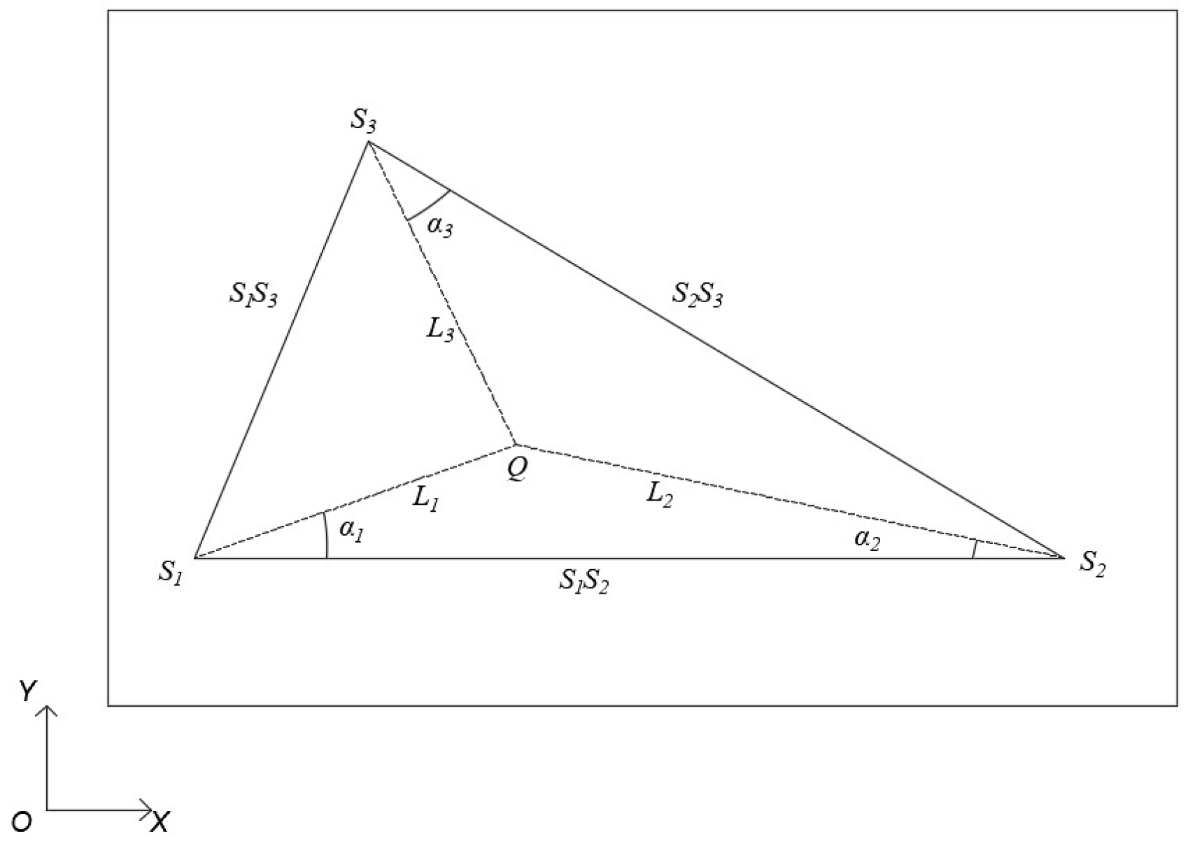
Triangulation localization: This is a position determination method based on triangular geometric relationships, which locates the target by measuring the distances between the target point and three known reference points. The method relies on trigonometric principles, such as the sum of interior angles theorem and the sine rule, to establish equations containing wave velocity and solve for the target position. In anisotropic structures, where wave velocity varies in different directions, an estimated average wave velocity can be used for calculations. The peak time of the signal processed by time-reversed virtual focusing is used to determine the arrival time of stress waves at each sensor. The arrival time differences between different sensors are then calculated based on the stress wave arrival times. Finally, the average wave velocity is estimated by fitting the slope of the line using the sensor spacing and arrival time differences, and this velocity value is used to replace the wave velocity in the anisotropic structure of the region. This is shown in Figure 4.

2.3. Localization Method Based on Energy Correlation

The principle of the localization method based on energy correlation is to theoretically establish a multiparameter linear model of the logarithmic value of sensor energy with respect to the relative positions between the sensor and the impact location. A minimization objective function is defined, and an optimization algorithm is used to solve for the value of this objective function, thereby providing the predicted impact source location [31,36]. The specific implementation process of this method is as follows:

(1)

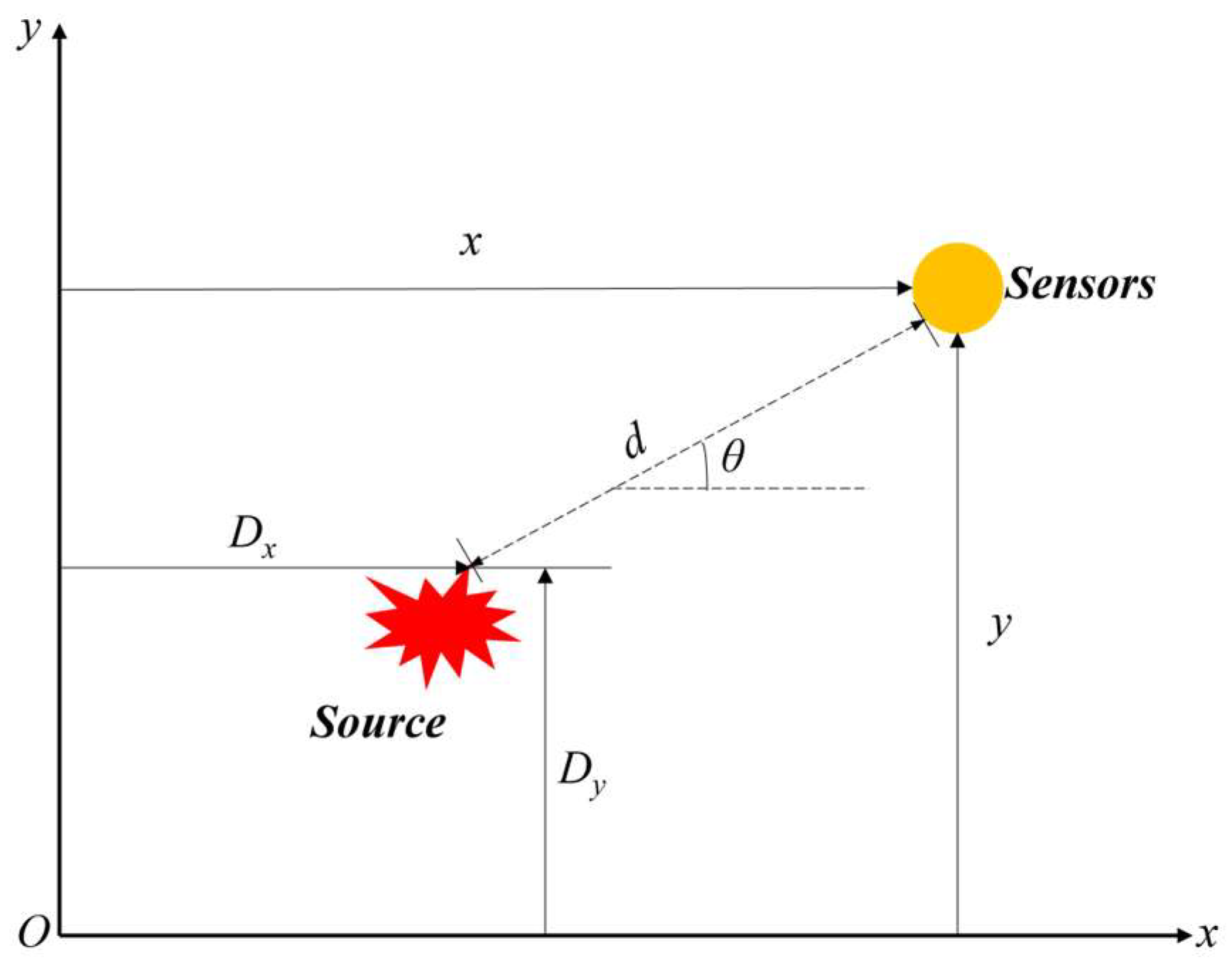
The relationship equation between the signal energy (E) and the relative position (relative distance d, relative angle θ) between the sensor and the impact position are established. The relative distance d is shown in Equation (7), the relative angle θ is shown in Equation (8), the relationship equation is shown in Equation (9), and the diagram is shown in Figure 5, as follows:

$$d=\sqrt{{(x-D_x)}^2+{(y-D_y)}^2}$$

(7)

$$\theta =\arctan \left|{\displaystyle \frac{y-D_y}{x-D_x}}\right|$$

(8)

$$\ln E=p+q\sqrt{{(x-D_x)}^2+{(y-D_y)}^2}+r\arctan \left|{\displaystyle \frac{y-D_y}{x-D_x}}\right|$$

(9)

where (D_x, D_y) represents the shock source position and (x, y) represents the sensor position. The derivation process of Equation (9) and the meanings of parameters are provided in Appendix A of the manuscript [31,36].

(2)

Combine the established relational equations to set the minimization objective function σ as shown in Equation (10).

$$\sigma ={\displaystyle \sum _{i=1}^n\left[\ln E_i-p\right.}-q\sqrt{{(x_i-D_x)}^2+{(y_i-D_y)}^2}{\left.-r\arctan \left|{\displaystyle \frac{y_i-D_y}{x_i-D_x}}\right|\right]}^2$$

(10)

(3)

This study employs an optimization algorithm to initialize algorithm parameters, including maximum iterations, population size, and variable dimensions. Initial positions of individuals are randomly assigned, with upper and lower bounds constrained by physical context. During the iterative process, corresponding fitness values are continuously calculated. The algorithm checks if the maximum iteration count is reached. If so, the optimization process terminates with the target value as the optimal solution. If not, iterations continue [37,38,39].

(4)

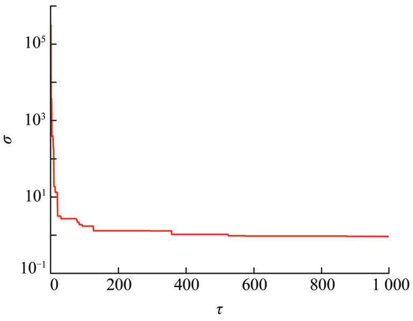
Upon reaching the convergence condition, the objective function σ value approaches its minimum, allowing for the determination of parameters D_x and D_y at this point, which serve as the predicted coordinates of the impact source location. In the localization method based on energy correlation proposed in this manuscript, the algorithm can be terminated when the convergence condition is met. The iterative curve of the objective function’s fitness value is shown in Figure 6. During the iterative process (where convergence typically begins around 10 iterations, with the convergence condition set at 1000 iterations), the objective function σ value progressively approaches its minimum. This yields the parameters D_x and D_y, which serve as predicted coordinates of the impact source location.

2.4. Evaluation of Localization Methods

Among these three localization methods, the method based on energy curvature and cumulative error primarily utilizes the energy curvature information of the time-domain signal. In contrast, the triangulation method based on time-reversed virtual focusing combines time-frequency domain information and leverages the temporal characteristics of the signal to determine the impact source location. Additionally, the localization method based on energy correlation enhances positioning accuracy by analyzing the correlation between signals. This method differs from the first two in that it does not directly utilize time-domain or frequency-domain information. The application contexts emphasized by different localization methods vary.

3. Experimental Verification

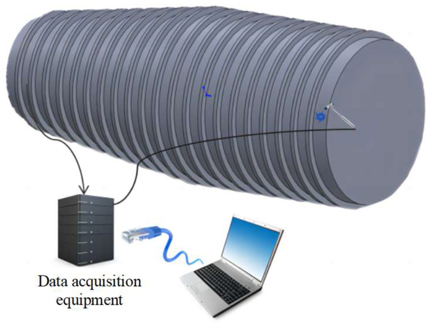
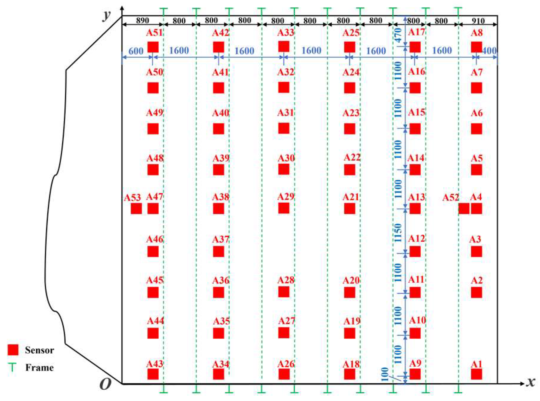
3.1. Experimental System and Sensor Layout

As shown in Figure 7, experiments were conducted on a ship’s stiffened cabin structure in this study. The cabin structure is made of Q235 material and has a cylindrical shell configuration with specific dimensions of diameter 3 m, length 9 m, and thickness 0.01 m. Impact responses were obtained by striking designated locations with an impact hammer and were captured by accelerometers. In this experiment, accelerometers on the ship cabin structure were arranged on one side of the cylindrical shell, and the impact tests were also performed on the same side. A total of 53 accelerometers were installed on the surface of the cabin structure, arranged circumferentially. The entire experimental testing system consists of the compartment model, accelerometers, impact hammer, data acquisition equipment, and a computer, as shown in Figure 8. The sampling frequency was 13,183 Hz. The hardware configuration of the computer was 12th Gen Intel (R) Core (TM) i7-12700H CPU @ 2.30 GHz @ 15.7 GB RAM. It was manufactured by Lenovo Group in Beijing, China. This study utilized Matlab 2021 software for analyzing experimental data results.

As shown in Figure 9, after unfolding the planar view of the ship cabin structure, the length in the horizontal axis direction is 9 m, and the length in the vertical axis direction is 9.42 m, with each rib spaced 0.80 m apart. The sensor located near the compartment door on the lower right side of the ship compartment model is named ‘A1’, with the remaining sensors numbered incrementally from bottom to top and from right to left. The green dashed lines in Figure 9 represent ribs, and the red square grid points represent the sensor measurement points. To simulate the actual operating environment of a ship and the sparse arrangement of measurement points, an impact localization experiment was conducted using a subset of sensors on the ship cabin structure, as shown in Figure 10. Figure 10 illustrates the distribution of impact points, with the blue ‘X’ marks indicating the positions of impacts.

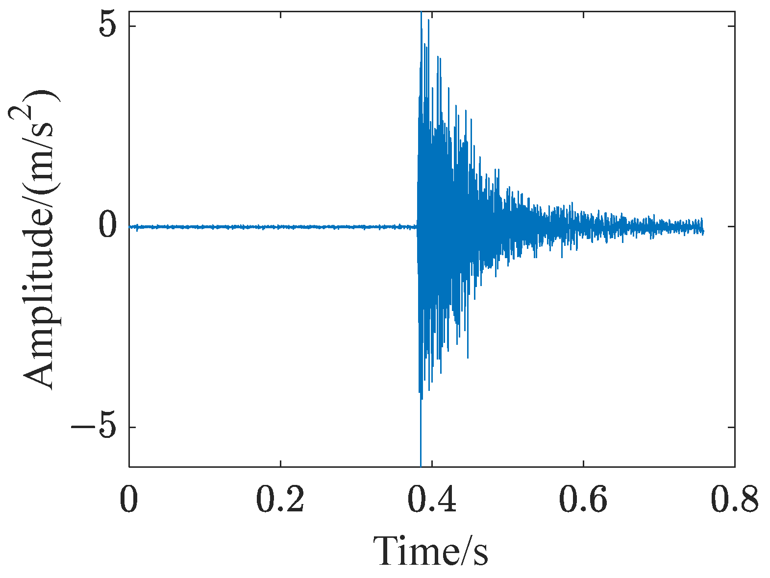
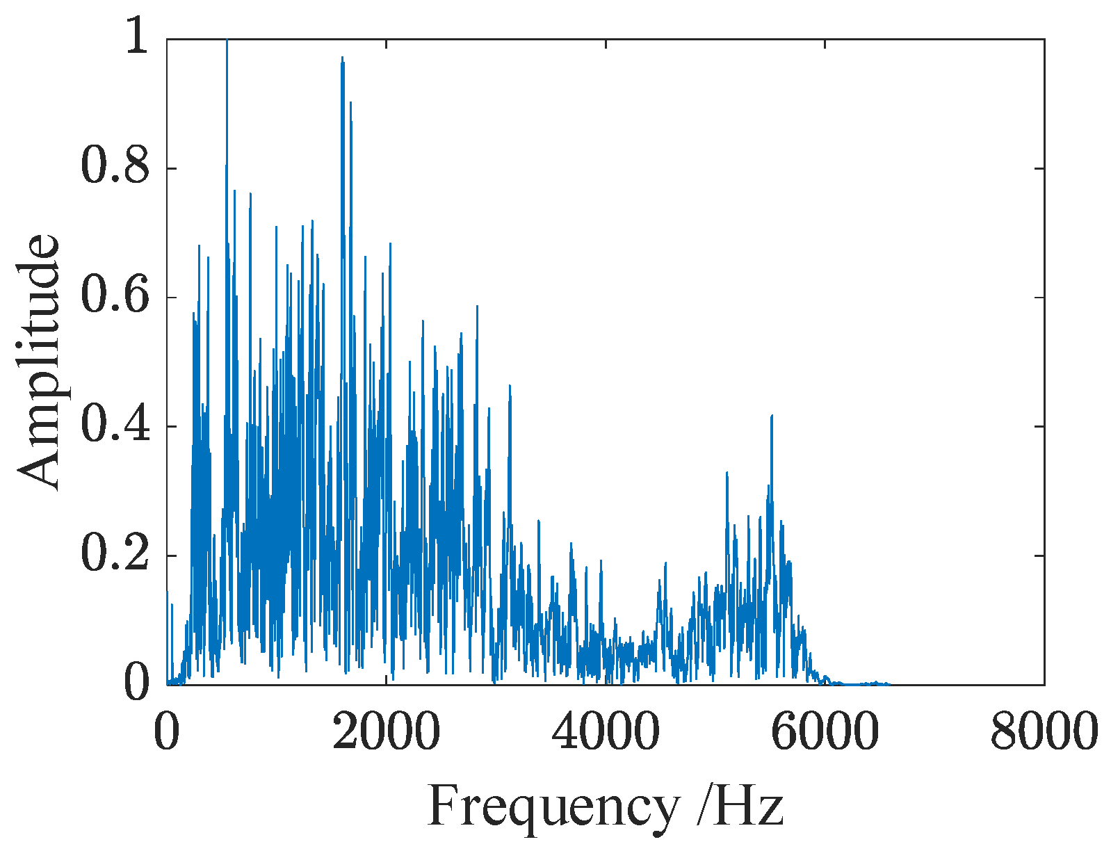
3.2. Signal Processing

When the first impact point location (K1) is subjected to an impact, the time-domain signal captured by sensor A1 is shown in Figure 11, and the frequency-domain signal is shown in Figure 12. Figure 11 and Figure 12 demonstrate that when a transient impact occurs in the ship cabin structure, the signal exhibits distinct pulse characteristics in the time domain. After excitation, due to the significant dispersion of wave propagation within the cabin structure, the frequency distribution of the signal appears more dispersed.

4. Elliptical Region-Based Localization Techniques

4.1. Representation of Elliptical Regions

As described previously, transient impact tests on the ship cabin structure can collect relevant sensor signal data. It is observed that each of the three localization methods—based on energy curvature and cumulative error, triangulation based on time-reversed virtual focusing, and energy correlation—provides a unique impact location coordinate. Thus, the three methods yield three distinct localization results. Consequently, this manuscript proposes an elliptical region-based localization strategy. This strategy defines an elliptical area to encompass all possible impact source locations and utilizes the results from multiple methods to narrow down this area, thereby achieving more precise localization. The specific calculation process is as follows:

First, calculate the mean coordinates $\overline{x}$, $\overline{y}$ and the standard deviations σ_x, σ_y of the three location coordinates. Then, with ($\overline{x}$, $\overline{y}$) as the center of the ellipse, construct an ellipse using three times the standard deviations 3σ_x and 3σ_y as the major and minor axes, respectively, based on the 3σ rule in statistics. The 3σ principle, also known as the ‘three standard deviation rule’, is a commonly used rule in statistics based on the properties of the normal distribution. The normal distribution is a symmetric, bell-shaped distribution with its mean (μ) at the center and the standard deviation (σ) measuring the dispersion of the data. The fundamental principle of the 3σ rule is that for a normally distributed dataset, approximately 99.73% of the data points fall within three standard deviations of the mean, i.e., within the interval [μ − 3σ, μ + 3σ]. This implies that if a data point falls outside this interval, it is likely to be an outlier, as there is less than a 0.27% probability of occurrence outside this range. The 3σ principle has widespread applications in quality control, anomaly detection, and other fields.

Finally, the elliptical region represents the actual predicted impact location area, as shown in Figure 13. This approach effectively reduces errors from different localization methods while narrowing the search range for the impact source and improving identification speed [40,41].

Therefore, based on the localization area obtained above, the error distance between the actual impact location and the elliptical localization area can be calculated. The specific method for calculating the error distance is as follows:

(1)

Parametric representation of the ellipse

First, parameterize the ellipse. For an ellipse centered at ($\overline{x}$, $\overline{y}$) with a major axis of length a (equal to 3σ_x) and a minor axis of length b (equal to 3σ_y), it can be parametrized as the following Equation (11).

$$\left\{\begin{array}{l}x=\overline{x}+a\cos \alpha \\ y=\overline{y}+b\sin \alpha \end{array}\right.$$

(11)

where α is a parameter ranging from 0 to 2π. Additionally, the boundary of the elliptical region can also be represented by a normalized equation, as shown in Equation (12).

$${\displaystyle \frac{{(x-\overline{x})}^2}{a^2}}+{\displaystyle \frac{{(y-\overline{y})}^2}{b^2}}=1$$

(12)

(2)

Distance from a point to the ellipse

As shown in Figure 14, assuming the actual impact location point P(x_real, y_real) is outside the elliptical region, the distance h to any point (x, y) on the ellipse can be expressed using the Euclidean distance as shown in Equation (13).

$$h=\sqrt{{(x-x_{real})}^2+{(y-y_{real})}^2}$$

(13)

(3)

Minimization of distance

Thus, when the impact location point P(x_real, y_real) is outside the elliptical region, the problem of Equation (13) can be transformed into finding the minimum value of h, as shown in Equation (14).

$$\min (h(\alpha ))=\min (\sqrt{{(\overline{x}+a\cos \alpha -x_{real})}^2+{(\overline{y}+b\sin \alpha -y_{real})}^2})$$

(14)

(4)

Distance calculation

To find the minimum value of h(α), the derivative of h(α) with respect to α can be taken and set to zero to solve for h(α). Additionally, numerical computation software can be used to determine the value of h(α), thereby calculating the distance.

(5)

Representation of error distance

When the actual impact location point P(x_real, y_real) is within the elliptical region, the error distance H should be represented as 0, as shown in Figure 14. According to Equation (12), if the coordinates of the impact location point P(x_real, y_real) satisfy the condition in Equation (15), it can be determined that the point is within the elliptical region.

$${\displaystyle \frac{{(x_{real}-\overline{x})}^2}{a^2}}+{\displaystyle \frac{{(y_{real}-\overline{y})}^2}{b^2}}\le 1$$

(15)

When the actual impact location point P(x_real, y_real) is outside the elliptical region, the error distance H is equal to the previously calculated distance h, as shown in Figure 15. According to Equation (12), if the coordinates of the impact location point P(x_real, y_real) satisfy the condition in Equation (16), it can be determined that the point is outside the elliptical region.

$${\displaystyle \frac{{(x_{real}-\overline{x})}^2}{a^2}}+{\displaystyle \frac{{(y_{real}-\overline{y})}^2}{b^2}}>1$$

(16)

4.2. Analysis and Discussion of Results

Based on the transient impact experiments conducted on the ship cabin structure, the range of the elliptical localization area and the error distances are presented in

Table 1. Localization result data.

Impact Point	$\overline{\mathit{x}}$/m	$\overline{\mathit{y}}$/m	σx/m	σy/m	3σx/m	3σy/m	xreal/m	yreal/m	h/m	H/m
I1	7.90	4.82	0.25	0.14	0.75	0.42	7.60	4.94	0.26	0.00
I2	8.03	4.88	0.38	0.63	1.14	1.89	7.60	5.24	0.68	0.00
I3	8.03	5.88	0.38	0.43	1.14	1.29	7.60	5.64	0.67	0.00
I4	6.85	4.35	0.20	0.40	0.60	1.20	6.80	3.95	0.51	0.00
I5	6.48	3.87	0.18	0.08	0.54	0.24	6.80	4.25	0.18	0.18
I6	7.21	5.10	0.29	0.15	0.87	0.45	6.80	4.94	0.23	0.00
I7	5.98	4.67	0.68	0.23	2.04	0.69	6.80	5.24	0.06	0.00
I8	6.08	5.27	0.78	0.68	2.34	2.04	6.80	5.64	1.42	0.00
I9	5.91	4.24	0.19	0.79	0.57	2.37	6.00	3.95	0.48	0.00
I10	5.68	4.09	0.38	0.14	1.14	0.42	6.00	4.25	0.24	0.00
I11	6.36	4.81	0.26	0.14	0.78	0.42	6.00	4.94	0.23	0.00
I12	6.31	5.37	0.21	0.09	0.63	0.27	6.00	5.24	0.10	0.00
I13	6.54	5.24	0.44	0.22	1.32	0.66	6.00	5.64	0.20	0.00
I14	5.68	5.30	0.23	0.00	0.69	0.00	5.20	4.94	0.36	0.36
I15	5.20	5.42	0.10	0.49	0.30	1.47	5.20	5.24	0.30	0.00
I16	5.30	5.10	0.00	0.85	0.00	2.55	5.20	5.64	0.10	0.10
I17	5.59	3.77	0.29	0.42	0.87	1.26	4.40	3.95	0.33	0.33
I18	4.98	4.58	0.48	0.23	1.44	0.69	4.40	4.25	0.30	0.00
I19	4.50	5.32	0.80	0.12	2.40	0.36	4.40	4.94	0.02	0.02
I20	4.90	5.01	0.40	0.45	1.20	1.35	4.40	5.24	0.67	0.00
I21	4.74	5.38	0.24	0.07	0.72	0.21	4.40	5.64	0.07	0.07
I22	3.58	5.39	0.48	0.09	1.44	0.27	3.60	4.94	0.18	0.18
I23	3.54	5.66	0.17	0.30	0.51	0.90	3.60	5.24	0.37	0.00
I24	3.96	5.95	0.54	0.01	1.62	0.03	3.60	5.64	0.28	0.28
I25	2.83	4.68	0.73	0.73	2.19	2.19	2.80	3.95	1.46	0.00
I26	2.01	5.31	0.19	0.01	0.57	0.03	2.80	4.25	1.08	1.08
I27	2.60	5.34	0.50	0.04	1.50	0.12	2.80	4.94	0.28	0.28
I28	2.50	5.18	0.40	0.27	1.20	0.81	2.80	5.24	0.71	0.00
I29	2.50	5.34	0.40	0.11	1.20	0.33	2.80	5.64	0.02	0.00
I30	1.44	4.22	0.67	0.27	2.01	0.81	2.00	3.95	0.50	0.00
I31	2.10	4.70	0.00	0.75	0.00	2.25	2.00	4.25	0.10	0.10
I32	2.10	4.90	0.00	0.06	0.00	0.18	2.00	4.94	0.10	0.10
I33	2.10	5.19	0.00	0.24	0.00	0.72	2.00	5.24	0.10	0.10
I34	1.80	5.69	0.30	0.09	0.90	0.27	2.00	5.64	0.21	0.00
I35	2.02	4.50	0.72	0.05	2.16	0.15	1.20	4.94	0.30	0.30
I36	1.73	5.01	0.37	0.05	1.11	0.15	1.20	5.24	0.10	0.10
I37	1.03	5.52	0.28	0.06	0.84	0.18	1.20	5.64	0.06	0.00

. As referenced earlier, ($\overline{x}$, $\overline{y}$) in Table 1 represents the center coordinates of the localization area, (σ_x, σ_y) represents the values of the standard deviations, (3σ_x, 3σ_y) represents three times the standard deviations, and (x_real, y_real) represents the true coordinates of the impact location. h represents the distance from the impact point to the elliptical region, while H represents the actual error distance value. The calculated values in Table 1 show that among the 37 actual impact locations, the average localization error distance is 0.10 m, indicating a low overall localization error that meets the required precision.

Specifically, the predicted locations of 22 impact points are within the localization area, with an error distance of 0. The predicted locations of 15 impact points are outside the localization area, among which 14 impact points have error distances ranging from 0 to 0.4 m, and 1 impact point has an error distance of 1.08 m. The distribution of transient impact localization error distances for the ship cabin structure is shown in Figure 16.

As shown in Table 1 and Figure 16, some impact locations exhibit larger error distances, which are analyzed below. Figure 17 illustrates typical signal characteristics of sensor A9 in different impact experiments. Figure 17a shows the signal of sensor A9 at impact point I1, which achieved high localization accuracy with an error distance of 0. In the experiment at impact point I1, sensor A9 received a strong impact wave signal despite not being very close to the impact point, primarily due to the strong connection between the sensor and the cabin structure. Figure 17b presents the signal of sensor A9 at impact point I17, where the localization algorithm begins to show errors with an error distance of 0.33 m. This is attributed to the weak connection between the sensor and the cabin structure, resulting in a weaker impact wave received by sensor A9 and the onset of localization errors. Figure 17c displays the signal of sensor A9 at impact point I26, where the localization error significantly increases. This is because the connection between the sensor and the cabin structure is even weaker, and accelerometer A9 fails to receive a sufficiently strong impact wave. The signal is also affected by multiple interfering pulse signals from the start of acquisition, further reducing the accuracy of impact localization. Consequently, the localization error for impact point I26 is larger, with an error distance of 1.08 m. All three signals in Figure 17 were collected under the same background conditions with roughly equal background noise levels. However, poor connections between the sensor and the cabin structure can lead to weaker received impacts and localization errors. Therefore, to avoid significant localization errors due to weak connections, data signals should be screened prior to each impact localization to exclude sensor data with anomalies, thereby enhancing the accuracy of impact source localization.

5. Conclusions

This manuscript presents an elliptical region-based localization strategy, which defines an elliptical area to encompass all possible impact source locations and integrates the results of different localization methods to narrow down this area, thereby achieving more precise localization.

The elliptical region localization strategy is based on these localization methods of energy curvature and cumulative error, time-reversed virtual focusing triangulation, and energy correlation, ultimately realizing the localization of transient impact sources in the ship cabin structure.

This study proposes an impact localization technique based on an elliptical region. The technique uses the arithmetic mean of the position coordinates obtained from three different localization methods as the center point and the three times standard deviations in the horizontal and vertical directions as the major and minor axes of the elliptical region, respectively, thereby constructing an elliptical localization area for precise regional impact localization.

The average error distance of the proposed impact localization technique in this study is 0.10 m. Through transient impact localization experiments on the ship cabin structure, it was found that the predicted positions of 22 impact points are all within the elliptical localization area, with an error distance of 0 m. While 15 impact points have predicted positions outside the elliptical localization area, among which 14 impact points have error distances ranging from 0 to 0.40 m, and 1 impact point has an error distance of 1.08 m. The primary reason for this is the insufficiently strong connection between the sensors and the cabin structure. Overall, the localization error remains at a low level, meeting the required precision.

The elliptical region-based impact source localization strategy proposed in the manuscript integrates multiple localization methods, transforming the traditional single-coordinate output mode into a regional localization mode and, thereby, effectively reducing errors. The strategy not only enhances the accuracy of localization but also strengthens the robustness of results, enabling it to better adapt to complex conditions in actual structures. The research outcomes of this manuscript provide a new technical approach for transient impact localization in the ship cabin structure and are expected to be promoted and applied in practical engineering.

References

1. Sikdar, S.; Mirgal, P.; Banerjee, S. Low-velocity Impact Source Localization in a Composite Sandwich Structure Using a Broadband Piezoelectric Sensor Network. Compos. Struct. 2022, 291, 115619. [Google Scholar] [CrossRef]
2. Goutaudier, D.; Osmond, G.; Gendre, D. Impact Localization on a Composite Fuselage with a Sparse Network of Accelerometers. Comptes Rendus Mec. 2020, 348, 191–209. [Google Scholar] [CrossRef]
3. Chen, B.; Hei, C.; Luo, M.; Ho, M.S.C.; Song, G. Pipeline Two-dimensional Impact Location Determination Using Time of Arrival with Instant Phase (Toaip) with Piezoceramic Transducer Array. Smart Mater. Struct. 2018, 27, 105003. [Google Scholar] [CrossRef]
4. Liu, J.; Hei, C.; Luo, M.; Yang, D.; Sun, C.; Feng, A. A Study on Impact Force Detection Method Based on Piezoelectric Sensing. Sensors 2022, 22, 5167. [Google Scholar] [CrossRef]
5. Liu, Q.; Wang, F.; Liu, M.; Xiao, W. A Two-step Localization Method Using Wavelet Packet Energy Characteristics for Low-velocity Impacts on Composite Plate Structures. Mech. Syst. Signal Process. 2023, 188, 110061. [Google Scholar] [CrossRef]
6. Zargar, S.A.; Yuan, F.G. Impact Diagnosis in Stiffened Structural Panels Using a Deep Learning Approach. Struct. Health Monit. 2020, 20, 681–691. [Google Scholar] [CrossRef]
7. Huang, J.; Wen, X.; Luo, J.; Luo, Q.; Long, Y.; Ren, L.; Liu, S. Localization Technique for Space Debris Impacted Spacecraft with PVDF Sensor. J. Astronaut. 2012, 33, 1341–1346. [Google Scholar]
8. Li, R.; Xu, R.; Cui, L.; Yu, W. Research and Application of Abnormal Noise Source Positioning Experiment Based on Double Cylindrical Shell. Chin. J. Ship Res. 2017, 12, 140–146. [Google Scholar]
9. Tobias, A. Acoustic-emission Source Location in Two Dimensions by an Array of Three Sensors. Non-Destr. Test. 1976, 9, 9–12. [Google Scholar] [CrossRef]
10. Ciampa, F.; Meo, M. Acoustic Emission Source Localization and Velocity Determination of the Fundamental Mode A0 Using Wavelet Analysis and a Newton-based Optimization Technique. Smart Mater. Struct. 2010, 19, 045027. [Google Scholar] [CrossRef]
11. Sabzevari, S.; Moavenian, M. Sound Localization in an Anisotropic Plate Using Electret Microphones. Ultrasonics 2017, 73, 114–124. [Google Scholar] [CrossRef] [PubMed]
12. Wang, G.; Chen, Y.; Li, B.; Guan, K. Composite Plate Damage Detection Method Based on Lamb Waves Probability Weighted Imaging. Noise Vib. Control 2023, 43, 149–156. [Google Scholar]
13. Wang, Q.; Yuan, S. No Baseline Time Reversal Imaging Method for Active Lamb Wave Structural Damage Monitoring. Chin. J. Aeronaut. 2010, 31, 178–183. [Google Scholar]
14. Coles, A.; Castro, B.D.; Andreades, C.; Baptista, F.G.; Meo, M.; Ciampa, F. Impact Localization in Composites Using Time Reversal Embedded PZT Transducers and Topological Algorithms. Front. Built Environ. 2020, 6, 27. [Google Scholar] [CrossRef]
15. Gorgin, R.; Wang, Z.; Wu, Z.; Yang, Y. Probability Based Impact Localization in Plate Structures Using an Error Index. Mech. Syst. Signal Process. 2021, 157, 107724. [Google Scholar] [CrossRef]
16. Peng, T.; Cui, L.; Huang, X.; Yu, W.; Xu, R. Error-index-based Algorithm for Low-velocity Impact Localization. Shock Vib. 2022, 2022, 2703789. [Google Scholar] [CrossRef]
17. Yang, L.; Deng, D.; Ma, S.; Xu, H.; Wu, Y.; Zhang, J. A Structural Impact Localization Method Based on Error Function. Patent CN202111296346.7, 29 October 2024. [Google Scholar]
18. Shi, C. Research on Impact Location Method of Composite Structures Based on Error Function. Master’s Thesis, Dalian Jiaotong University, Dalian, China, 2023. [Google Scholar]
19. Yang, L.; Deng, D.; Tian, G.; Gao, Z.; Bao, X.; Wu, Z. Probabilistic Imaging Impact Localization on Composite Stiffened Plate Based on Error Function. J. Vib. Meas. Diagn. 2024, 44, 88–93+199. [Google Scholar]
20. Han, W.; Feng, K.; Luo, Y. Hyperbolic Location Damage Imaging Method Based on Ultrasonic Lamb Wave. Nondestruct. Test. 2021, 43, 46–50. [Google Scholar]
21. Yan, S.; Li, B. Impact Localization of Thin Plate Structures Using PZT-array Based Passive Wave Method. IOP Publ. 2019, 283, 012040. [Google Scholar] [CrossRef]
22. Yin, S. Study of Acoustic Source Localization Techniques Based on TDOA. Ph.D. Thesis, Jilin University, Changchun, China, 2020. [Google Scholar]
23. Su, Y.; Yuan, S.; Zhou, H. Impact Localization in Composite Using Two-step Method by Triangulation Technique and Optimization Technique. J. Astronaut. 2009, 30, 1201–1206. [Google Scholar]
24. Yan, S. The Impact Detection and Crack Identification Technology Based on the Active and Passive Method Integration. Master’s Thesis, Wuhan University, Wuhan, China, 2019. [Google Scholar]
25. Migot, A.; Giurgiutiu, V. Impact Localization Using Sparse PWAS Networks and Wavelet Transform. Struct. Health Monit. Int. J. 2017, 391–398. [Google Scholar] [CrossRef]
26. Zhao, W.; Xu, X.; Song, R.; Yang, M.; Qi, C. Research on Noise Source Locating for Car Door Rattle Based on Time Reversal Method. Automot. Eng. 2022, 44, 1954–1963. [Google Scholar]
27. Qi, T.; Chen, Y.; Li, X.; Lu, C.; Li, Q. An Acoustic Emission Source Location Method Based on Time Reversal for Glass Fiber Reinforced Plastics Plate. Chin. J. Sci. Instrum. 2020, 41, 208–217. [Google Scholar]
28. Wu, Z.; Zeng, X.; Deng, D.; Yang, Z.; Yang, H.; Ma, S.; Yang, L. Impact Localization on Stiffened Composite Plate Based on Adaptive Time Reversal Focusing. Acta Mater. Compos. Sin. 2024, 41, 507–520. [Google Scholar]
29. Yu, W.; Xu, R.; Huang, X.; Wu, S.; Peng, T. A Structural Impact Localization Method Based on Energy Curvature and Cumulative Error. Patent CN202310686775.8, 5 September 2023. [Google Scholar]
30. Huang, X.; Xu, R.; Yu, W.; Wu, S. Impact Localization in Complex Cylindrical Shell Structures Based on The Time-reversal Virtual Focusing Triangulation Method. Sensors 2024, 24, 5185. [Google Scholar] [CrossRef]
31. Huang, X.; Xu, R.; Yu, W.; Cui, L.; Cheng, G. Impact Source Localization Method Based on Energy Correlation under Multiscale Models. J. Huazhong Univ. of Sci. Tech. 2024, 52, 127–134+184. [Google Scholar]
32. Cai, J.; Shi, L.; Yuan, S. High Resolution Damage Imaging of Composite Plate Structures Based on Virtual Time Reversal. J. Compos. Mater. 2012, 29, 183–189. [Google Scholar]
33. De Simone, M.E.; Ciampa, F.; Meo, M. A Hierarchical Method for the Impact Force Reconstruction in Composite Structures. Smart Mater. Struct. 2019, 28, 085022. [Google Scholar] [CrossRef]
34. Yu, Z.; Xu, C.; Sun, J.; Du, F. Impact Localization and Force Reconstruction for Composite Plates Based on Virtual Time Reversal Processing with Time-Domain Spectral Finite Element Method. Struct. Health Monit. 2023, 22, 4149–4170. [Google Scholar] [CrossRef]
35. Qiu, L.; Yuan, S.; Zhang, X.; Wang, Y. A Time Reversal Focusing Based Impact Imaging Method and Its Evaluation on Complex Composite Structures. Smart Mater. Struct. 2011, 20, 105014. [Google Scholar] [CrossRef]
36. Sen, N.; Kundu, T. A New Signal Energy-based Approach to Acoustic Source Localization in Orthotropic Plates: A Numerical Study. Mech. Syst. Signal Process. 2022, 171, 108843. [Google Scholar] [CrossRef]
37. Jalalah, M.; Hua, L.G.; Hafeez, G.; Ullah, S.; Alghamdi, H.; Belhaj, S. An Application of Heuristic Optimization Algorithm for Demand Response in Smart Grids with Renewable Energy. AIMS Math. 2024, 9, 14158–14185. [Google Scholar] [CrossRef]
38. Hua, L.G.; Ali Shah, S.H.; Alghamdi, B.; Hafeez, G.; Ullah, S.; Murawwat, S.; Ali, S.; Khan, M.I. Smart Home Load Scheduling System with Solar Photovoltaic Generation and Demand Response in the Smart Grid. Front. Energy Res. 2024, 12, 1322047. [Google Scholar] [CrossRef]
39. Alghamdi, H.; Khan, T.A.; Hua, L.G.; Hafeez, G.; Khan, I.; Ullah, S.; Khan, F.A. A Novel Intelligent Optimal Control Methodology for Energy Balancing of Microgrids with Renewable Energy and Storage Batteries. J. Energy Storage 2024, 90, 111657. [Google Scholar] [CrossRef]
40. Ghorpade, S.; Zennaro, M.; Chaudhari, B. Survey of Localization for Internet of Things Nodes: Approaches, Challenges and Open Issues. Future Internet 2021, 13, 210. [Google Scholar] [CrossRef]
41. Gao, F.; An, J.; Wu, Y. Impact analysis of platform positioning and orientation error on warship weapon target strike. Evol. Intell. 2024, 17, 171–176. [Google Scholar]
Figure 1. Scene diagram of impact localization action.
Jmse 13 00333 g001
Figure 2. Diagram of impact localization probability imaging.
Jmse 13 00333 g002
Figure 3. Schematic diagram of time-reversal virtual focusing.
Jmse 13 00333 g003
Figure 4. Triangle localization diagram.
Jmse 13 00333 g004
Figure 5. Diagram of impact source and relative position of sensor.
Jmse 13 00333 g005
Figure 6. Iterative change curve of objective function value.
Jmse 13 00333 g006
Figure 7. Real diagram of impact test system.
Jmse 13 00333 g007
Figure 8. Schematic diagram of impact test system.
Jmse 13 00333 g008
Figure 9. Schematic diagram of the plan expansion of the ship cabin structure (dimensions in mm).
Jmse 13 00333 g009
Figure 10. Diagram of impact location.
Jmse 13 00333 g010
Figure 11. Time domain diagram.
Jmse 13 00333 g011
Figure 12. Normalized frequency domain diagram.
Jmse 13 00333 g012
Figure 13. Representation of the elliptical localization area.
Jmse 13 00333 g013
Figure 14. The actual impact point is outside the localization area.
Jmse 13 00333 g014
Figure 15. The actual impact point is within the localization area.
Jmse 13 00333 g015
Figure 16. Distribution diagram of impact localization error distance.
Jmse 13 00333 g016
Figure 17. Signal captured by accelerometer A9 in the impact test: (a) point I1; (b) point I17; (c) point I26.
Jmse 13 00333 g017