Numerical Analysis on the Scale Effect of a Free-Running Ship’s Manoeuvring Characteristics

Abstract

This study focuses on the manoeuvring characteristics of model- and full-scale ships. Various methods, including free-running model tests (FRMTs), computational fluid dynamics (CFD), and theoretical approaches, were employed to estimate ship manoeuvring performance. However, these methods are typically simulated at model-scale, which introduces discrepancies in the Reynolds number due to Froude scaling laws. Although numerous studies have investigated scale effects, most have concentrated on ship resistance, with limited research on manoeuvring performance. To address this gap, this study developed a free-running CFD simulation model for both a model-scale and full-scale ONRT. The study involved a detailed analysis of manoeuvring trajectories, forces, and moments. This analysis aimed to highlight differences in manoeuvring performance caused by Reynolds number discrepancies between model- and full-scale ships, providing a quantitative assessment of performance variations across scales and contributing to a more accurate understanding of manoeuvring characteristics at full scale.

1. Introduction

The manoeuvring performance of a ship is crucial for safe and efficient operations. A recent study found that navigational accidents, including collisions and groundings, account for over 40% of all maritime incidents [1]. These accidents often stem from improper manoeuvring by navigation officers. Therefore, understanding a ship’s manoeuvring performance in actual sea conditions is vital for ensuring safety at sea.

For a better understanding of the manoeuvring characteristics of a ship, several methods have been proposed to estimate a ship’s manoeuvrability, including free-running model tests (FRMTs), computational fluid dynamics (CFD), and theoretical methods. FRMTs are the most robust methods for evaluating manoeuvring characteristics. They are intuitive and accurate. Many experiments have been conducted using real-time control and communication systems [2,3,4,5,6,7]. However, FRMTs require large basins, costly facilities, skilled technicians, and so on. Thus, only a few facilities are capable of conducting FRMTs. As an alternative, outdoor FRMTs using the Global Positioning System (GPS) have been proposed [8]. While this method has showed reliable results, external forces from wind and currents may have affected the test outcomes.

Traditionally, theoretical methods combine mathematical models with potential flow theory to predict ship manoeuvring characteristics. The most representative method, the manoeuvring mathematical group (MMG) model, simulates ship manoeuvring in three degrees of freedom (3-DOF; surge, sway, and yaw). These methods offer short computational times and align well with experimental data, leading to numerous studies [9,10,11,12,13,14,15,16,17]. However, 3-DOF models do not account for roll, pitch, and heave. To address these limitations, Seo and Kim (2011) used a 4-DOF model that included roll [18]. Kim et al. (2024) further assessed the turning ability of two ships, with and without a bulbous bow, in calm seas and waves. They found differences in manoeuvring performance based on ship speed, wavelength, and bulbous bow presence [19]. Nevertheless, the inability to address all 6-DOF remains an issue, leaving errors related to pitch and heave unresolved. Additionally, potential flow theory’s inability to account for viscous effects reduces prediction accuracy [20].

Recently, CFD has emerged as an alternative tool for estimating a ship’s manoeuvrability. Previously, CFD had disadvantages due to high computational costs. However, advancements in computer technology have reduced time costs and improved accuracy. This approach is now an attractive tool for researchers, leading to a considerable number of studies [21,22,23,24,25,26,27,28,29]. In particular, CFD methods can incorporate both viscous and rotational effects in the flow, accurately resolving the complex fluid–structure interactions. Research in this area has demonstrated the excellence of direct CFD methods for estimating a ship’s manoeuvrability in calm water by comparing CFD results with available experimental data.

Numerical simulations in the aforementioned methods are performed at a model scale to replicate the conditions of related experimental fluid dynamics (EFD) tests, following Froude scaling laws. This approach results in notable discrepancies in the Reynolds number when compared with full-scale ships, raising concerns about the precision of these model-scale measurements when extrapolated to full-scale ships. To address this issue, extensive research has been conducted on scale effects. For example, A. Dogrul et al. (2020) investigated the impact of scale on resistance components and form factors using the KRISO Container Ship (KCS) and KRISO Very Large Crude Carrier (KVLCC2), noting effects on flow characteristics, wave patterns, and resistance components [30]. Kim et al. (2021) conducted numerical simulations using virtual fluid at a model scale to predict full-scale propeller performance [31]. Terziev et al. (2022) published a review paper of studies exploring the scale effect of ship hydrodynamics [32]. Similarly, Kim et al. (2024) conducted a numerical study to predict full-scale ship resistance, examining performance and flow structure using virtual fluid and validating these against real fluid conditions [33]. While many studies have addressed scale effects, the majority have concentrated on ship resistance, with fewer studies examining manoeuvring characteristics.

To the best of the authors’ knowledge, no CFD-based study has addressed the scale effects of ship manoeuvring. Therefore, the present study aimed to fill this gap by developing a free-running manoeuvre model based on the URANS method.

In this study, a free-running CFD simulation model was developed for a benchmark ship hull of a surface combatant, the Office of Naval Research Tumblehome (ONRT, DTMB 5613). The computational domain of the simulation model incorporated multiple levels of a dynamic overset grid system, which solved the ship’s motion and rudder manipulations. The body-force propeller method was employed to simulate the flow around the hull and rudder of the self-propelled ONRT. Simulations were carried out for the following two different ship scales: model-scale and full-scale ships. Full-scale simulations were conducted using the following two different approaches: scaled simulations and simulations using virtual fluid. The virtual fluid approach adjusted the viscosity in model-scale simulations to match the Reynolds number of the full-scale scenario. Numerical manoeuvring tests (e.g., zigzag and turning circle tests) were conducted to analyse differences in manoeuvring characteristics between model- and full-scale ships by comparing manoeuvring trajectories and decomposing the forces and moments involved.

2. Methodology

2.1. Governing Equation

The proposed CFD model was developed based on the Reynolds-averaged Navier–Stokes (RANS) method using a commercial CFD software package, STAR-CCM+ ver 18.06. As in the following two equations, the averaged continuity and momentum equations for incompressible flows may be given in tensor notation and Cartesian coordinates [34].

$${\displaystyle \frac{\partial \left(\rho u_i\right)}{\partial x_i}}=0,$$

(1)

$$\rho {\displaystyle \frac{\partial \left(u_i\right)}{\partial t}}+\rho u_j{\displaystyle \frac{\partial u_i}{\partial x_j}}=-{\displaystyle \frac{\partial P}{\partial x_i}}+{\displaystyle \frac{\partial }{\partial x_j}}\left(2\mu S_{ij}-\rho \overline{u_i^{\prime }{u}_j^{\prime }}\right),$$

(2)

$$S_{ij}={\displaystyle \frac{1}{2}}\left({\displaystyle \frac{\partial u_i}{\partial x_j}}+{\displaystyle \frac{\partial u_j}{\partial x_i}}\right)$$

(3)

$$\rho {\tau }_{\mathrm{i}\mathrm{j}}=-\rho \overline{u_i^{\prime }{u}_j^{\prime }}$$

(4)

where the $\rho$ is the density, $u$ is the averaged velocity vector, $P$ is the averaged pressure, $\mu$ is the dynamic viscosity, $-\rho \overline{u_i^{\prime }{u}_j^{\prime }}$ is known as the Reynolds-stress tensor, $S_{ij}$ is a strain-rate tensor, and ${\tau }_{ij}$ is the specific Reynolds-stress tensor.

The computational domains were discretised and solved using a finite volume method within the CFD solver. For the momentum equations, a second-order upwind convection scheme and a first-order temporal discretisation were utilised. The overall solution process was based on a pressure-linked equation (SIMPLE)-type algorithm, which integrated the continuity and momentum equations to achieve a predicted velocity field that satisfied the continuity equation through pressure correction. For the free surface of the simulation, the volume of fluid (VOF) method was employed with high-resolution interface capturing (HRIC).

The turbulent flow was simulated using the shear stress transport (SST) $\kappa$-$\omega$ turbulence model. This model is a hybrid of the $\kappa$-$ϵ$ and $\kappa$-$\omega$ models, contributing to more accurate calculations.

2.2. Coordinate System

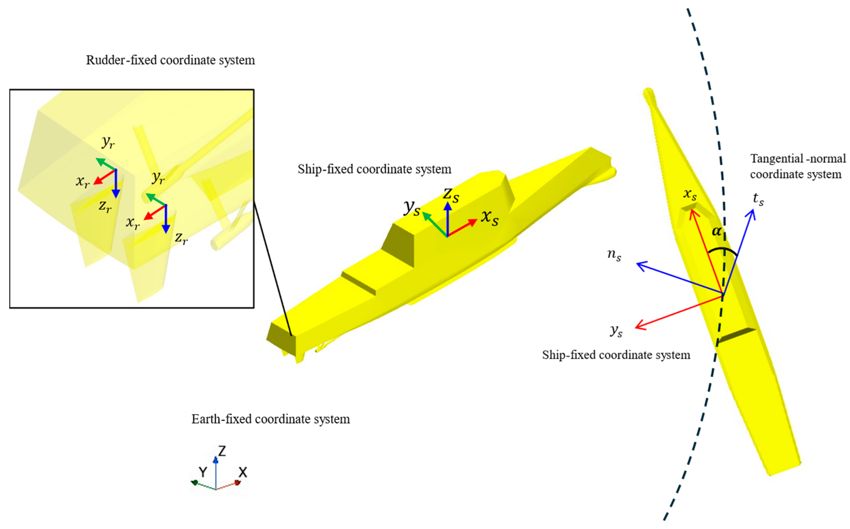
Figure 1 illustrates the coordinate system of the ship used in this study. The ship experienced slip during its manoeuvring, which occurred due to the difference between the direction of movement and the ship’s heading. This phenomenon primarily arises from the lateral motion caused by a ship’s turning manoeuvre and is a significant factor that reduces the vessel’s manoeuvring efficiency. As a result, the direction in which the bow is pointing and the actual trajectory of the ship do not align. To account for this, the drift angle was calculated using $v_x$ and $v_y$, obtained relative to the ship-fixed coordinate system, and the transformation to the tangential–normal (t-n) coordinate system was performed by rotating the axis accordingly.

2.3. Geometry and Boundary Conditions

This study utilised both a model-scale and full-scale Office of Naval Research Tumblehome (ONRT, DTMB 5613). The model-scale ONRT was employed to validate the experimental data. Figure 2 illustrates the hull geometry of the vessel, while

Table 1. Principal particulars and conditions of the ONR Tumblehome adapted from SIMMAN 2020.

		Full-Scale	Model-Scale
Scale factor	$\lambda$	1	48.9355
Length of waterline	$L_{WL}$ (m)	154.0	3.147
Beam at waterline	$B_{WL}$ (m)	18.78	0.384
Depth	$D$ (m)	14.5	0.266
Design draft	$T$ (m)	5.494	0.112
Displacement	$∆$	8507 ton	72.6 kg
Wetted surface area (fully appended)	$S$ (m2)	N/A	1.5
Block coefficient	$C_B$	0.535	0.535
Longitudinal centre of buoyancy	LCB (%), aft of FP	N/A	1.625
Metacentric height	GM (m)	N/A	0.0422
Radius of gyration for roll	$k_{xx}/B$	0.444	0.444
Radius of gyration for yaw	$k_{yy}/L_{wl}$; $k_{zz}/L_{wl}$	0.25	0.246
Max. rudder turn rate	${\dot{\delta }}_{max}$ (°/s)	5.0	35.0

represents the principal particulars.

Figure 3 shows the computational domain and boundary conditions used in the simulation. The domain was represented as a block, with dimensions of 5.5 L in length, 3 L in width, and 4 L in height. A velocity inlet boundary condition was applied to the upstream face (positive x-direction), the side boundaries (the two opposite faces along the y-direction), and the top and bottom surfaces of the domain. The downstream face (negative x-direction) was defined using a pressure outlet condition. 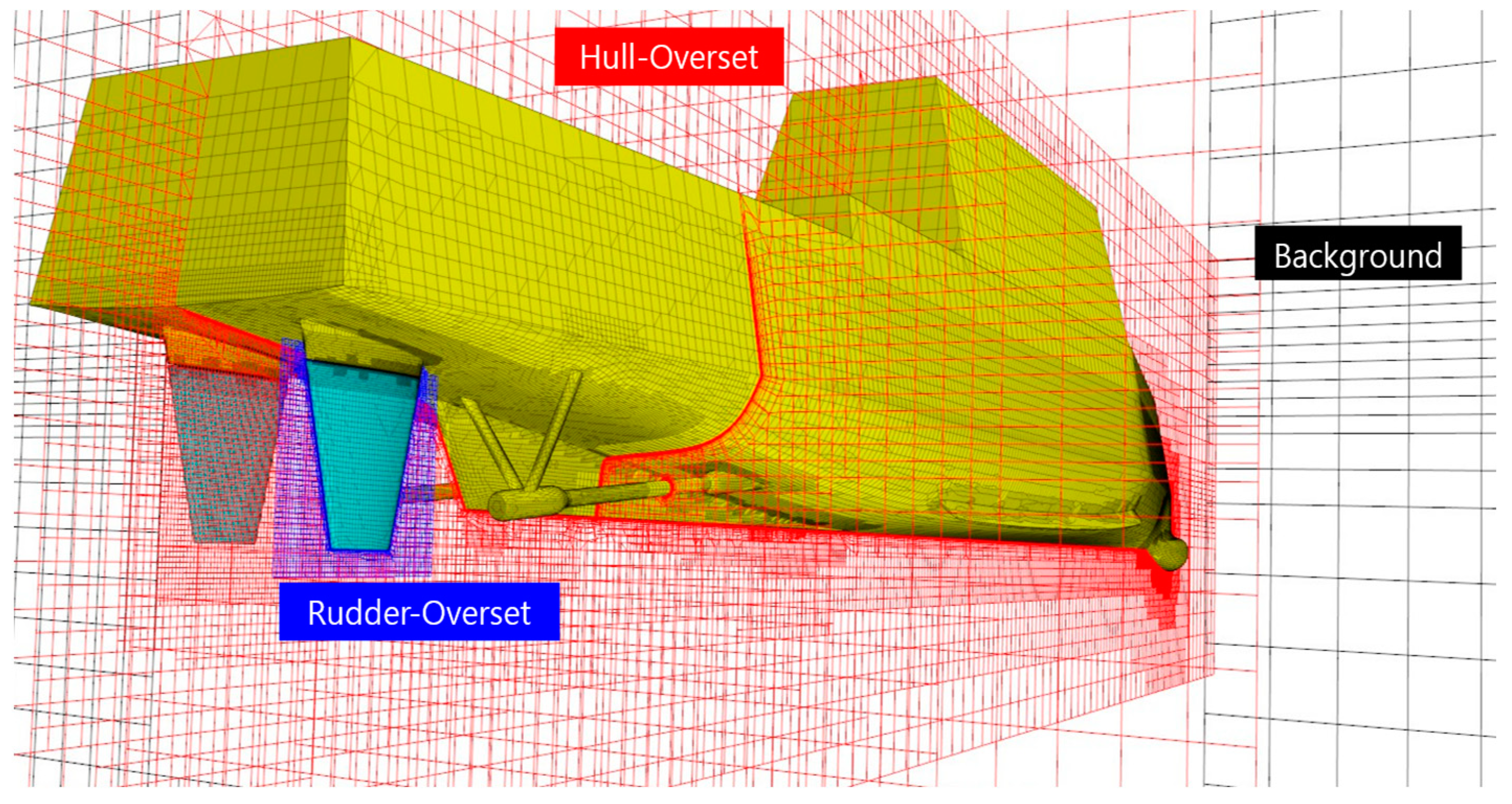Figure 4 depicts the multi-level dynamic overset grid system. In this system, the background domain was designed to adhere to the ONRT model, allowing for three degrees of freedom (3-DOF) in motion; specifically, surge, sway, and yaw. The hull-overset domain, on the other hand, supported six degrees of freedom (6-DOF) for the motion of the ship. Additionally, within the hull-overset, the rudder-overset grid included superimposed rudder movements, complementing the 6-DOF hull motion to accurately simulate rudder manipulation.

2.4. Body-Force Propeller

This section describes the body-force propeller method utilised in this study. The propeller model was developed based on the specifications and open-water data supplied by the Iowa Institute of Hydraulic Research (IIHR).

Table 2. The main particulars of the propeller model.

	Full-Scale	Model-Scale ($\mathit{\lambda }$ = 48.9355)
Type	FP	FP
No. of blades	4	4
Diameter	5.2165	0.1066
Rotation	Inwards	Inwards
Hub ratio	0.20	0.20

and

Table 3. Parameters of body-force propeller method.

Item	Applied Method/Value
Virtual disk method	Body-force propeller method
Propeller curve	Open-water data from IIHR
Thrust/torque specification	Goldstein’s optimum distribution
Thickness	0.1 D
Radial distribution option: thrust and torque	Same distribution
Inflow specification method	Inflow velocity plane
Inflow plane radius	1.1 D
Inflow plane offset	0.05 D
Induced velocity correction	Enabled

outline the key details of the propeller model and the parameters applied to the body-force propeller model.

2.5. Mesh Generation

Mesh generation was performed using the STAR-CCM+ mesh tool. Trimmed cell meshes were used to express high-quality fine meshes for complex domains. In addition, local refinements were used to improve mesh quality in critical areas such as the area around the hull and the Kelvin wake area. For critical areas, meshes were generated that were approximately 2 to 4 times finer than the mesh size in regions farther from the hull. In particular, a refined prism layer was applied to effectively capture the changes in the velocity gradient around the hull.

In this study, the model-scale ship was set with a $y^{+}$ value of less than 1, while the full-scale ship was set with a value of approximately 300. Therefore, prism-layer meshes were used for near-wall refinement, and the thickness of the first-layer cell on the surface was set to satisfy the $y^{+}$ value [29]. Grids were generated to achieve the same resolution for both the model-scale and full-scale ships. The $y^{+}$ value, commonly around 300 for full-scale ships, was matched, and the prism-layer settings were adjusted to ensure a fair comparison between the model-scale and full-scale ships (i.e., stretch factor, total thickness, etc.). Figure 5 shows the volume meshes of the domain.

Table 4. Numerical conditions for simulation cases.

	Model-Scale	Ship (Virtual Fluid)	Ship (Scaled)
$F_n$	0.20
$R{e}_L$	$2.75\times {10}^6$	$9.42\times {10}^8$	$9.42\times {10}^8$
No. of grids	2,837,374	2,871,770	2,866,339
$y^{+}$	1	300	300

presents the conditions of the simulation cases used in this study. As mentioned above, simulations were conducted for model- and full-scale ships, with full-scale simulations using scaled and virtual fluid approaches. The virtual fluid method adjusted the viscosity to match the full-scale Reynolds number.

2.6. Controller

To achieve a self-propelled state with a zero-heading angle, the ship’s propeller rotation speed and rudder angle were controlled. This was accomplished using the propeller and rudder control systems outlined below.

2.6.1. Propeller Controller

To ascertain the vessel’s target speed, a proportional–integral (PI) controller, similar to the one implemented by Song et al. (2024) [28], was utilised. The primary distinction lay in the specific control gain values used. Notably, the propeller controller was employed solely during the self-propulsion phase as the zigzag and turning manoeuvres were carried out using a fixed n value. Consequently, the selection of control gains did not influence the outcomes of the manoeuvring simulations. However, optimising the control gains could significantly reduce the computation time required for the self-propulsion simulations. Figure 6 presents the time history of the vessel’s speed and the propeller’s rotational speed as self-propulsion was established. To reach the design speed of 1.110 m/s, the propeller rotational speed was calculated to be n = 8.86 rps. This value slightly differed from the experimental data reported by IIHR, where $n_{EFD}$ was measured as 8.97 rps, resulting in a relative deviation of approximately 1.2%.

2.6.2. Rudder Controller

To determine the neutral rudder angle required for maintaining a zero-heading angle, a proportional–integral–differential (PID) controller was employed, as utilised by Song et al. (2024) [28]. Like the propeller controller, the difference lay in the control gain values, which did not affect the results of the simulation, only the time cost. Figure 7 shows the time history of the rudder and heading angles as self-propulsion with a zero-heading angle was attained. The neutral rudder angle was obtained as ${\delta }_N$ = 0.04°. For twin-screw ships, a neutral rudder angle is typically 0 degrees due to their symmetric design. Although the current study showed a slight deviation of 0.04 degrees from neutral, this could be attributed to numerical error. Such minor variations commonly arise from small asymmetries in the volumetric mesh generation during simulation. For the zigzag and turning circle manoeuvres, the rudder was controlled to follow the target rudder angles without exceeding the maximum rudder rate.

3. Results

3.1. V&V

3.1.1. Verification Study

A verification study was performed to ensure that the proper grid spacing and time step were set. A discretisation error estimation was performed based on the Richardson extrapolation [35]. As stated in [3], the final formulation for the fine-grid convergence index is presented in Equation (5), as follows:

$$GC{I}_{fine}^{21}={\displaystyle \frac{1.25e_a^{21}}{r_{21}^{P_a}-1}}$$

(5)

where $e_a^{21}$ is the approximate relative error of the key variables.

$$e_a^{21}=\left|{\displaystyle \frac{{\phi }_1-{\phi }_2}{{\phi }_1}}\right|$$

(6)

Here, $r_{21}$ is the refinement factor given by $r_{21}=\sqrt[3]{N_1/N_2}$, where $N_1$ and $N_2$ are the fine and medium cell numbers, respectively. The apparent order of the method, $p_a$, is determined by solving Equations (7) and (8) iteratively, as follows:

$$P_a={\displaystyle \frac{1}{\ln \left(r_{21}\right)}}\left|ln\left|{\displaystyle \frac{{\epsilon }_{32}}{{\epsilon }_{21}}}\right|+q\left(p_a\right)\right|$$

(7)

$$q\left(p_a\right)=\mathrm{l}\mathrm{n}({\displaystyle \frac{r_{21}^{p_a}-s}{r_{32}^{p_a}-s}})$$

(8)

where $s=sign\left({\displaystyle \frac{{\epsilon }_{32}}{{\epsilon }_{21}}}\right)$, ${\epsilon }_{32}={\phi }_3-{\phi }_2$, ${\epsilon }_{21}={\phi }_2-{\phi }_1$, and $r_{32}$ is the refinement factor given by $r_{21}=\sqrt[3]{N_2/N_3}$, where $N_3$ is the coarse cell number. The extrapolated value of the key variables is calculated by Equation (9).

$${\phi }_{ext}^{21}={\displaystyle \frac{r_{21}\left({\phi }_1-{\phi }_2\right)}{r_{21}-1}}$$

(9)

The extrapolated relative error, $e_{ext}^{21}$, is obtained by Equation (10).

$$e_{ext}^{21}=\left|{\displaystyle \frac{{\phi }_{ext}^{21}-{\phi }_1}{{\phi }_{ext}^{21}}}\right|$$

(10)

Table 5. Uncertainty estimations from spatial and temporal convergence test. Key variable: $Transfer/L_{pp}$.

Model-Scale ($\mathit{\lambda }=48.9355$)
	Spatial Convergence	No. of Cells	$\mathit{T}\mathit{r}\mathit{a}\mathit{n}\mathit{s}\mathit{f}\mathit{e}\mathit{r}/{\mathit{L}}_{\mathit{p}\mathit{p}}$	Temporal Convergence	$∆\mathit{t}\left(\mathit{s}\right)$	$\mathit{T}\mathit{r}\mathit{a}\mathit{n}\mathit{s}\mathit{f}\mathit{e}\mathit{r}/{\mathit{L}}_{\mathit{p}\mathit{p}}$
Fine		2,871,770	1.25096		0.01	1.259081
Medium		1,429,763	1.568833		0.02	1.25096
Coarse		644,777	1.570602		0.04	1.204942
	$GC{I}_{Fine}^{21}(\%)$		0.0750	$GC{I}_{∆t_2}^{32}(\%)$		0.9854

shows the results of the spatial and temporal convergence study of the ONRT simulation. The spatial and temporal uncertainties were calculated based on the fine mesh and fine time step for each case. This study used the fine mesh and fine time step for accurate results.

3.1.2. Validation Study

The validation study was conducted by comparing the 35° portside turning circle manoeuvre and 20°/20° zigzag manoeuvre trajectory from the CFD simulation with the model test data of IIHR provided for the SIMMAN 2020 workshop. Figure 8, Figure 9, Figure 10 and Figure 11 illustrate the turning circle and zigzag trajectories for both the ONRT simulations and the model test results from IIHR. The simulation outcomes demonstrated excellent alignment with the experimental data. Figure 8 depicts the turning circle trajectories for the 35° portside turning circle manoeuvre obtained from the CFD simulation and the EFD data. The CFD result showed a great agreement of trajectory with the EFD data.

Table 6. Derived characteristics for the circle manoeuvre obtained from CFD and EFD data.

	CFD	EFD	Difference (%)
Transfer/$L_{PP}$	1.25	1.34	−6.64
Advance/$L_{PP}$	2.37	2.35	0.86
Tactical diameter/$L_{PP}$	3.15	3.19	−1.42

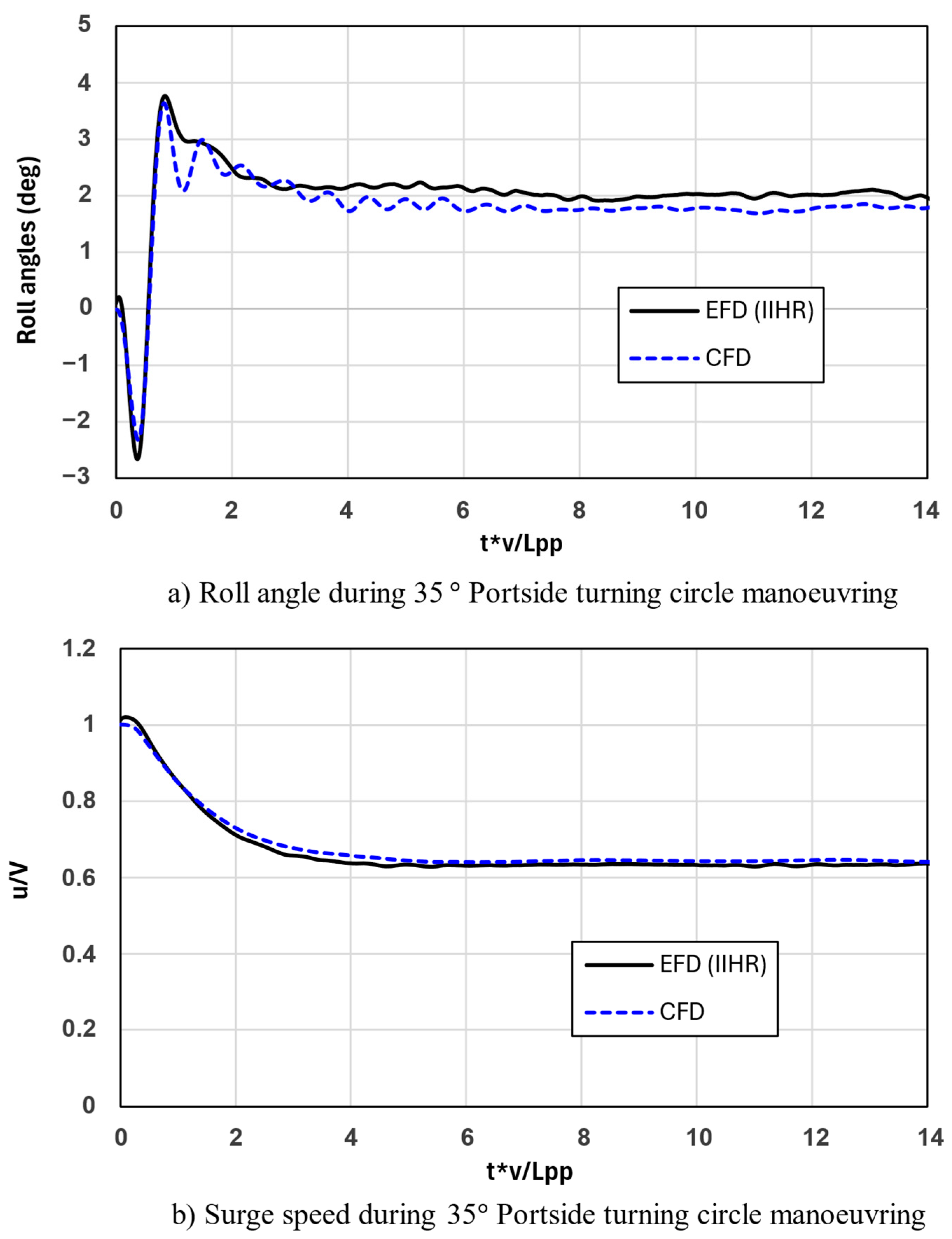
presents the turning circle manoeuvring characteristics of CFD and EFD. Figure 9a,b present a comparison between the CFD predictions and the EFD data for the roll angles and surge speeds, respectively, during the manoeuvres.

Figure 10 shows the 20°/20° zigzag manoeuvre trajectory from the CFD simulation and the model test data of IIHR. It depicted great agreement compared with the EFD trajectory. Figure 11a,b present a comparison of the CFD predictions with the EFD data for the roll angles and surge speeds, respectively, during the manoeuvres. The exceptions were an underestimation of roll angles during the zigzag manoeuvre and an overestimation of speed reduction during the turning circle manoeuvre.

4. Results

The forces and moments acting on a vessel during manoeuvring performance, especially the turning and zigzag manoeuvres, are very closely related. This relationship is a key factor in determining how a vessel responds to a given manoeuvring command and how efficiently it can follow the desired course.

The forces and moments acting on a turning vessel are longitudinal and lateral forces, the yawing moment, and propulsive force. Longitudinal and lateral forces arise from the pressure and resistance of the water on the hull and rudder, influenced by the rudder angle, causing the ship to follow a curved path. The yawing moment is generated because this lateral force acts at a distance from the ship’s centre of gravity, including rotation and determining the turning radius. Lastly, propulsive force plays a crucial role in maintaining the ship’s speed. In the Results section, the differences in manoeuvring trajectories are analysed by comparing the forces and moments between the model-scale and full-scale ships.

4.1. The 35° Portside Turning Circle Manoeuvre

Figure 12 illustrates the comparison of turning circle trajectories during the 35° portside turning circle manoeuvre under various scales obtained from CFD data. As shown in Figure 12, the turning trajectory for the model-scale ship was found to be smaller than that for the full-scale ship. To analyse these results, the ship speed as well as the x- and y-axis forces on the hull and rudder (portside and starboard) during the turning manoeuvre were examined. All the forces and moments were non-dimensionalised for a clearer comparison, and the equations used are as follows:

$${\displaystyle \frac{Force}{\frac{1}{2}\rho V^{2}LT}}$$

(11)

$${\displaystyle \frac{Moment}{\frac{1}{2}\rho V^2{L}^{2}T}}$$

(12)

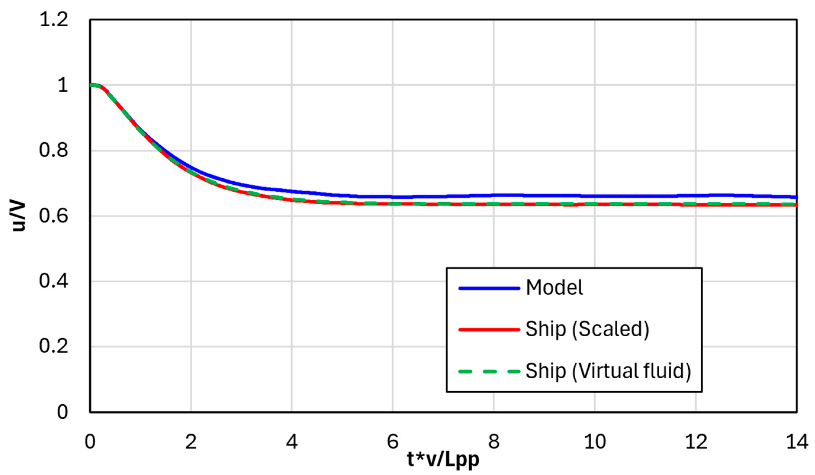
4.1.1. Ship Speed

First of all, to analyse the cause of the difference in turning circle trajectories, the ship’s speed was examined. As shown in Figure 13, the model-scale surge speed converged higher than the ship-scale surge speed (3.9%). Higher terminal speeds lead to a larger centrifugal force during a turning circle manoeuvre, resulting in larger turning circles [28]. A more detailed analysis of the reason why the ship speed converged to a higher one in the model-scale ship is conducted in the following section.

4.1.2. Longitudinal and Lateral Forces

To analyse the ship speed, an analysis of the forces acting on the ship was conducted. The longitudinal and lateral forces (i.e., x- and y-dir.) were examined using the ship-fixed coordinate system, especially the total net force of the x- and y-axis forces. The total net forces included the hull drag, rudder drag, and thrust force in each direction. For a better understanding, we compared the forces obtained by rotating this system by an angle of drift into the t-n coordinate system (see Figure 1). Figure 14 illustrates the drift angles during the turning circle manoeuvre. The drift angles, α, were calculated using Equation (13).

$$\alpha =\mathrm{a}\mathrm{r}\mathrm{c}\mathrm{t}\mathrm{a}\mathrm{n} ({\displaystyle \frac{v_y}{v_x}})$$

(13)

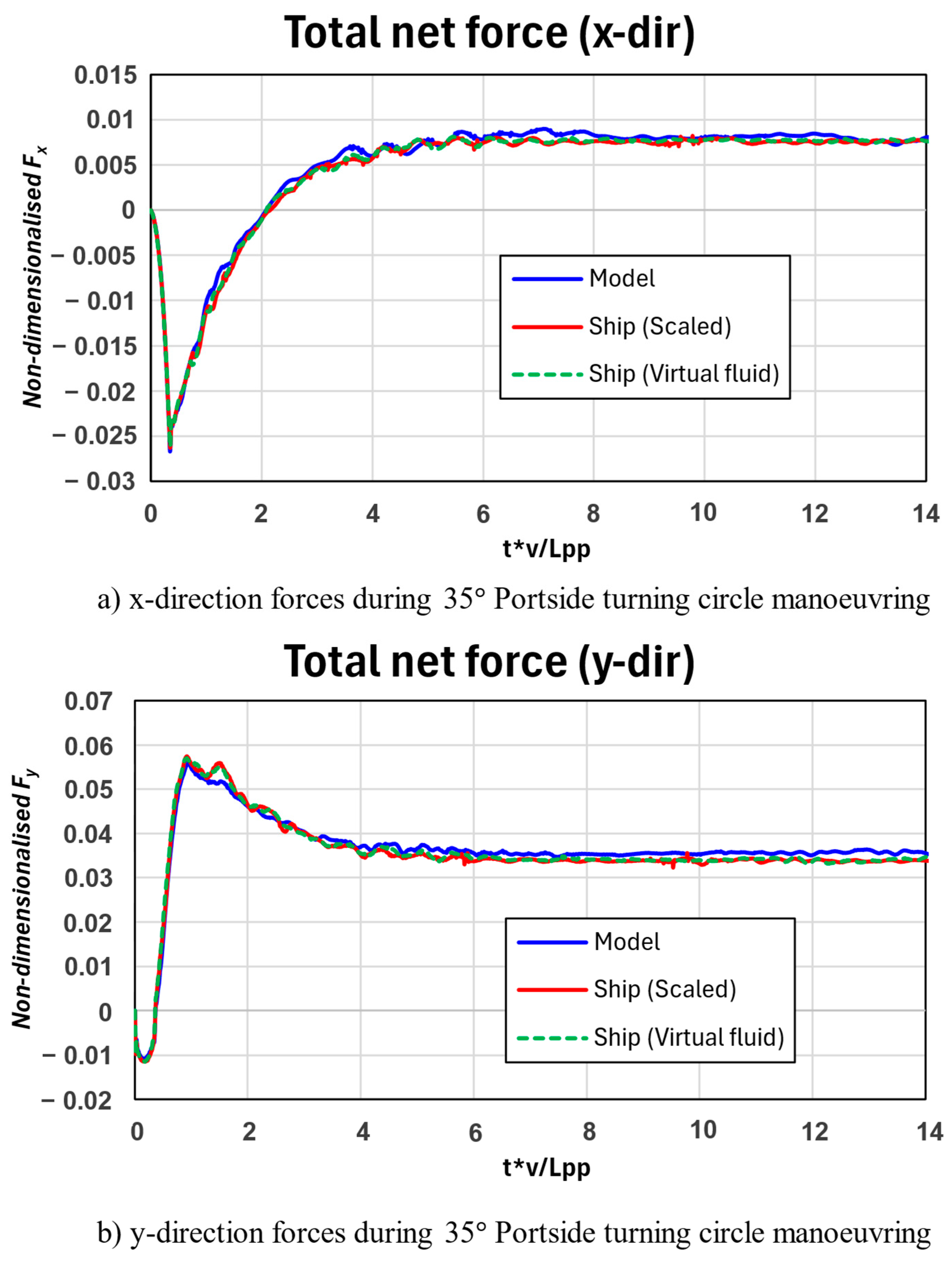
Figure 15 depicts the x-direction and y-direction total net forces of the model-scale and full-scale ships. The total net forces included the hull drag, rudder drag, and thrust force in each direction. As shown in Figure 15, the total net force for the model-scale ship was greater than the full-scale ship.

Figure 16 illustrates the t- and n-directional total net forces for the model-scale and full-scale ships. The solid line in Figure 16a represents the non-dimensionalised $F_t$, while the dashed line depicts its cumulative integral. As the results of the ship (scaled) and ship (virtual fluid) showed remarkable similarity, the following figure focuses on comparing and analysing the model and ship (scaled) cases for better readability. To provide a more quantitative comparison, the t-directional forces during the turning manoeuvre were integrated and compared. As shown in Figure 16a, the cumulative integral amounts during the turning manoeuvre were $4.63\times {10}^{-2}$ for the model and $4.92\times {10}^{-2}$ for the ship (scaled), indicating that the ship (scaled) experienced approximately 6.38% greater values. This suggests that the model experienced less backward force compared with the ship (scaled); consequently, it converged to a higher surge speed. Figure 16b illustrates the n-directional total net force. As depicted in Figure 16b, a higher terminal speed was observed in the model-scale ship, resulting in a larger $F_n$ for the model-scale ship.

4.1.3. Yawing Moment

Figure 17 shows the z-axis moment (yawing moment) for both scales. For a clearer understanding, the cumulative integral of the z-moment is shown with a dashed line. As shown in Figure 17, a larger z-moment was observed for the ship (scaled). As the z-moment, also referred to as the yawing moment, increases, the vessel experiences a stronger turning force. This increase in turning force allows the ship to execute turns more effectively. Consequently, the vessel can turn within a narrower radius compared with when the yawing moment is lower, effectively reducing the turning radius.

4.2. The 20°/20° Portside Zigzag Manoeuvre

Figure 18 illustrates the comparison of 20°/20° zigzag manoeuvre trajectories across two different scales (i.e., model-scale and full-scale ships) obtained from CFD data. As seen in Figure 18, the overshoot angles for the model were smaller than those for the ship (scaled) and the overall trajectory shifted to the right. To analyse these results, similar to the turning manoeuvre, the ship speed and the x- and y-axis forces on the hull and rudder (portside and starboard) during the zigzag manoeuvre were examined. These forces and moments were non-dimensionalised for comparison in accordance with Equations (11) and (12).

4.2.1. Ship Speed

As shown in Figure 19, the model converged to a higher speed compared with the ship (scaled). As noted by Song et al. (2024a) [20], smaller surge speeds are associated with larger overshoot angles. Similarly, the model, which exhibited a higher surge speed, demonstrated smaller overshoot angles, whereas the ship (scaled), with a lower surge speed, showed larger overshoot angles. However, the differences observed were smaller when compared with those of the turning circle manoeuvre. This analysis continues in the following section.

4.2.2. Longitudinal and Lateral Forces

Similar to the previous turning circle manoeuvre, the zigzag manoeuvre also involved converting the x and y forces into t-n forces according to the drift angle, as shown in Figure 20 for a better understanding. Figure 21 and Figure 22 illustrate the x and y forces as well as the converted t and n forces, respectively.

The dashed line in Figure 22a illustrates the cumulative integral of $F_t$ during the zigzag manoeuvre. It was observed that the cumulative integral of $F_t$ in the model ($4.35\times {10}^{-2}$) was smaller than that of the ship (scaled) ($4.69\times {10}^{-2}$). This indicated that the model experienced less deceleration and, consequently, converged to a larger surge speed (u/V). However, the degree of difference observed was smaller compared with that in the turning circle manoeuvre. Furthermore, as shown in Figure 22b, the n-directional force, $F_n$, of the ship (scaled) was larger than that of the model. This indicated that the side force acting on the ship (scaled) was greater, which could be expected to result in a larger overshoot.

4.2.3. Yawing Moment

Figure 23 shows the z-moment acting on the vessel during the zigzag manoeuvre. As shown in the figure, the z-moment was more pronounced in the ship (scaled) compared with the model. A larger z-moment results in a stronger rotation of a vessel, which is evident in Figure 18 where the slope of the yaw angle is steeper for the ship (scaled) than for the model. However, a stronger z-moment can lead to the rapid rotation of a vessel, potentially increasing the overshoot angle. Consequently, a larger overshoot angle was observed for the ship (scaled) compared with the model.

5. Conclusions

With the aim of investigating the scale effect on a free-running ship, we conducted a URANS analysis with the benchmark ship hulls of a surface combatant, ONR Tumblehome. To confirm the scale effect on a free-running ship, we developed the following two different ship scales: model-scale and full-scale ships. Full-scale simulations were carried out using two approaches, a scaled simulation (i.e., ship (scaled)) and a simulation using virtual fluid (i.e., ship (virtual fluid)).

Spatial and temporal convergence studies were conducted using the grid convergence index (GCI) method to estimate the numerical uncertainties of the proposed CFD models and to determine appropriate grid spacing and time steps, while for the validation of the simulation, model-scale ONRT Tumblehome 35° portside turning circle and 20°/20° zigzag manoeuvres were conducted. The results of the trajectories obtained from the simulation showed great agreement with the experimental data from IIHR provided for the SIMMAN 2020 workshop.

Remarkably, the results of the 35° portside turning circle manoeuvre clearly demonstrated a pronounced scale effect between the model-scale and the full-scale ships. Due to differences in the tangential forces acting on the vessel during motion, the speed of the full-scale ship decreases more, leading to a lower velocity and, consequently, a smaller turning radius. Additionally, the larger yawing moment observed for the full-scale ship contributed to a reduced turning radius.

In the case of the 20°/20° zigzag manoeuvre, a similar difference due to the scale effect was present for the model-scale and full-scale ships. As with the turning circle manoeuvre, the difference in tangential forces resulted in a lower terminal speed in the full-scale ship. However, the extent of this difference was less pronounced compared with the turning manoeuvre. Nevertheless, due to the slower speed and larger z-moment, a greater overshoot angle was observed for the full-scale ship, along with a steeper slope in the vessel’s yaw angle.

As a result, both the model- and full-scale ships maintained a net zero force in the self-propulsion state, with forces in the x-axis direction being dominant. However, the model-scale ship experienced greater drag, particularly frictional resistance, due to the difference in the Reynolds number, which required a larger thrust for the model-scale ship. As the manoeuvre began and lateral forces came into play, the model-scale ship experienced greater drag than the full-scale ship. Nevertheless, the larger thrust compensated for this, leading to a greater convergence of surge speed for the model-scale ship.

This study investigated the scale effect caused by differences in Reynolds numbers in free-running vessels. The vessel used in this study was a twin-screw slender-body warship, which exhibited small roll and small overshoot angles. However, other merchant vessels tend to show relatively larger roll and overshoot angles, with differences in their manoeuvring trajectories. Essentially, greater roll is expected to result in larger gravitational forces, which can induce a more significant scale effect. Therefore, future research should investigate the scale effect on other types of ships (i.e., container ships, tankers, etc.).

References

- EMSA. Annual Overview of Marine Casualties and Incidents 2020; EMSA: Lisbon, Portugal, 2020. [Google Scholar]
- Stern, F.; Toxopeus, S.; Visonneau, M.; Guilmineau, E.; Lin, W.-M.; Grigoropoulos, G. CFD, potential flow, and system-based simulations of course keeping in calm water and seakeeping in regular waves for 5415M. In Proceedings of the NATO AVT-189 Meeting, Fareham, UK, 12–14 October 2011. [Google Scholar]
- Araki, M.; Sadat-Hosseini, H.; Sanada, Y.; Tanimoto, K.; Umeda, N.; Stern, F. Estimating maneuvering coefficients using system identification methods with experimental, system-based, and CFD free-running trial data. Ocean Eng. 2012, 51, 63–84. [Google Scholar] [CrossRef]
- Kim, D.J.; Yun, K.; Park, J.-Y.; Yeo, D.J.; Kim, Y.G. Experimental investigation on turning characteristics of KVLCC2 tanker in regular waves. Ocean Eng. 2019, 175, 197–206. [Google Scholar] [CrossRef]
- Sanada, Y.; Elshiekh, H.; Toda, Y.; Stern, F. ONR Tumblehome course keeping and maneuvering in calm water and waves. J. Mar. Sci. Technol. 2019, 24, 948–967. [Google Scholar] [CrossRef]
- Sanada, Y.; Tanimoto, K.; Takagi, K.; Gui, L.; Toda, Y.; Stern, F. Trajectories for ONR Tumblehome maneuvering in calm water and waves. Ocean Eng. 2013, 72, 45–65. [Google Scholar] [CrossRef]
- Yun, K.; Choi, H.; Kim, D.J. An experimental study on the manoeuvrability of KCS with different scale ratios by free running model test. J. Soc. Nav. Arch. Korea 2021, 58, 415–423. [Google Scholar] [CrossRef]
- Park, J.; Lee, D.; Park, G.; Rhee, S.H.; Seo, J.; Yoon, H.K. Uncertainty assessment of outdoor free-running model tests for maneuverability analysis of a damaged surface combatant. Ocean Eng. 2022, 252, 111135. [Google Scholar] [CrossRef]
- Skejic, R.; Faltinsen, O.M. A unified seakeeping and maneuvering analysis of ships in regular waves. J. Mar. Sci. Technol. 2008, 13, 371–394. [Google Scholar] [CrossRef]
- Zhang, W.; Zou, Z.-J.; Deng, D.-H. A study on prediction of ship maneuvering in regular waves. Ocean Eng. 2017, 137, 367–381. [Google Scholar] [CrossRef]
- Yasukawa, K.; Kino, S.; Ohta, J.; Azami, K.; Tanaka, E.; Mimura, K.; Fujinaga, K.; Nakamura, K.; Kato, Y. Stratigraphic variations of fe–mn micronodules and implications for the formation of extremely rey-rich mud in the western north pacific ocean. Minerals 2021, 11, 270. [Google Scholar] [CrossRef]
- Lee, J.; Nam, B.W.; Lee, J.-H.; Kim, Y. Development of Enhanced Two-Time-Scale Model for Simulation of Ship Maneuvering in Ocean Waves. J. Mar. Sci. Eng. 2021, 9, 700. Available online: https://www.mdpi.com/2077-1312/9/7/700 (accessed on 25 June 2021). [CrossRef]
- Atasayan, E.; Milanov, E.; Alkan, A.D. Application of an offline grey box method for predicting the manoeuvring performance. Brodogradnja 2024, 75, 75304. [Google Scholar] [CrossRef]
- Jambak, A.I.; Bayezit, I. Robust optimal control of a nonlinear surface vessel model with parametric uncertainties. Brodogr. Int. J. Nav. Archit. Ocean Eng. Res. Dev. 2023, 74, 131–143. [Google Scholar] [CrossRef]
- Li, Y.; Tang, Z.; Gong, J. The effect of PID control scheme on the course-keeping of ship in oblique stern waves. Brodogradnja 2023, 74, 155–178. [Google Scholar] [CrossRef]
- Liang, L.; Zhao, P.; Zhang, S.; Yuan, J. Simulation analysis of fin stabilizers on turning circle control during ship turns. Ocean Eng. 2019, 173, 174–182. [Google Scholar] [CrossRef]
- Sano, M. Mathematical model and simulation of cooperative manoeuvres among a ship and tugboats. Brodogradnja 2023, 74, 127–148. [Google Scholar] [CrossRef]
- Seo, M.-G.; Kim, Y. Numerical analysis on ship maneuvering coupled with ship motion in waves. Ocean Eng. 2011, 38, 1934–1945. [Google Scholar] [CrossRef]
- Kim, B.-S.; Kim, Y.; Yang, H.; Kim, T.; Kim, J. Analysis of turning ability of large tankers with and without bulbous bow in calm sea and waves. Appl. Ocean Res. 2024, 148, 104002. [Google Scholar] [CrossRef]
- Mofidi, A.; Carrica, P.M. Simulations of zigzag maneuvers for a container ship with direct moving rudder and propeller. Comput. Fluids 2014, 96, 191–203. [Google Scholar] [CrossRef]
- Kim, D.; Song, S.; Sant, T.; Demirel, Y.K.; Tezdogan, T. Nonlinear URANS model for evaluating course keeping and turning capabilities of a vessel with propulsion system failure in waves. Int. J. Nav. Arch. Ocean Eng. 2022, 14, 100425. [Google Scholar] [CrossRef]
- Kim, D.; Yim, J.; Song, S.; Demirel, Y.K.; Tezdogan, T. A systematic investigation on the manoeuvring performance of a ship performing low-speed manoeuvres in adverse weather conditions using CFD. Ocean Eng. 2022, 263, 112364. [Google Scholar] [CrossRef]
- Kim, D.; Yim, J.; Song, S.; Park, J.-B.; Kim, J.; Yu, Y.; Elsherbiny, K.; Tezdogan, T. Path-following control problem for maritime autonomous surface ships (MASS) in adverse weather conditions at low speeds. Ocean Eng. 2023, 287, 115860. [Google Scholar] [CrossRef]
- Li, H.; Zhao, N.; Zhou, J.; Chen, X.; Wang, C. Uncertainty Analysis and Maneuver Simulation of Standard Ship Model. J. Mar. Sci. Eng. 2024, 12, 1230. [Google Scholar] [CrossRef]
- Li, J.; Wang, Q.; Dong, K.; Wang, X. Numerical Simulations of a Ship’s Maneuverability in Shallow Water. J. Mar. Sci. Eng. 2024, 12, 1076. [Google Scholar] [CrossRef]
- Kinaci, O.K.; Ozturk, D. Straight-ahead self-propulsion and turning maneuvers of DTC container ship with direct CFD simulations. Ocean Eng. 2021, 244, 110381. [Google Scholar] [CrossRef]
- Song, S.; Kim, D.; Dai, S. CFD investigation into the effect of GM variations on ship manoeuvring characteristics. Ocean Eng. 2024, 291, 116472. [Google Scholar] [CrossRef]
- Wang, J.; Wan, D. CFD investigations of ship maneuvering in waves using naoe-FOAM-SJTU Solver. J. Mar. Sci. Appl. 2018, 17, 443–458. [Google Scholar] [CrossRef]
- Wang, J.; Zou, L.; Wan, D. Numerical simulations of zigzag maneuver of free running ship in waves by RANS-Overset grid method. Ocean Eng. 2018, 162, 55–79. [Google Scholar] [CrossRef]
- Dogrul, A.; Song, S.; Demirel, Y.K. Scale effect on ship resistance components and form factor. Ocean Eng. 2020, 209, 107428. [Google Scholar] [CrossRef]
- Kim, K.-W.; Paik, K.-J.; Lee, J.-H.; Song, S.-S.; Atlar, M.; Demirel, Y.K. A study on the efficient numerical analysis for the prediction of full-scale propeller performance using CFD. Ocean Eng. 2021, 240, 109931. [Google Scholar] [CrossRef]
- Terziev, M.; Tezdogan, T.; Incecik, A. Scale effects and full-scale ship hydrodynamics: A review. Ocean Eng. 2022, 245, 110496. [Google Scholar] [CrossRef]
- Kim, K.-W.; Paik, K.-J.; Lee, S.-H.; Lee, J.-H.; Kwon, S.-Y.; Oh, D. A numerical study on the feasibility of predicting the resistance of a full-scale ship using a virtual fluid. Int. J. Nav. Arch. Ocean Eng. 2024, 16, 100560. [Google Scholar] [CrossRef]
- Wilcox, D.C. Turbulence Modeling for CFD, 3rd ed.; Dcw Industries: La Cañada Flintridge, CA, USA, 2006. [Google Scholar]
- Celik, I.B.; Ghia, U.; Roache, P.J.; Freitas, C.J.; Coleman, H.; Raad, P.E. Procedure for Estimation and Reporting of Uncertainty Due to Discretization in CFD Applications. J. Fluids Eng. 2008, 130, 078001. [Google Scholar] [CrossRef]
Figure 1.
The coordinate system of the ship used in this study.
Figure 2.
Geometry of the benchmark ship hull of a navy surface combatant, ONRT.
Figure 3.
Computation domain and boundary conditions of ONRT simulation.
Figure 4.
Multi-level overset grid system.
Figure 5.
Volume mesh generation.
Figure 6.
Time history of the propeller rotation speed and ship speed for self-propulsion computation.
Figure 7.
Time history of rudder angle and heading angle for self-propulsion computation.
Figure 8.
Trajectories of the 35 portside turning circle manoeuvre obtained from CFD and EFD data.
Figure 9.
(a,b) Roll angles and surge speeds during the 35 portside turning circle manoeuvres obtained from CFD and EFD data.
Figure 10.
Trajectories of the 20/20 portside zigzag manoeuvre obtained from CFD and EFD data.
Figure 11.
(a,b) Roll angles and surge speeds during the 20°/20° portside zigzag manoeuvre obtained from CFD and EFD data.
Figure 12.
Trajectory comparison of the 35 portside turning circle manoeuvre obtained from CFD data.
Figure 13.
Surge speed comparison of the 35 portside turning circle manoeuvre obtained from CFD data.
Figure 14.
Drift angles during the 35 portside turning circle manoeuvre obtained from CFD data.
Figure 15.
(a,b) Total net forces (x-dir. and y-dir.) of the 35 portside turning circle manoeuvre obtained from CFD data.
Figure 16.
(a,b) Total net forces (t-dir. and n-dir.) of the 35 portside turning circle manoeuvre obtained from CFD data.
Figure 17.
Total z-moment of the 35 portside turning circle manoeuvre obtained from CFD data.
Figure 18.
Trajectory comparison of the 20/20 zigzag manoeuvre obtained from CFD data.
Figure 19.
Surge speed comparison of the 20/20 zigzag manoeuvre obtained from CFD data.
Figure 20.
Drift angles during the 20/20 zigzag manoeuvre obtained from CFD data.
Figure 21.
(a,b) Total net forces (x-dir. and y-dir.) of the 20/20 zigzag manoeuvre obtained from CFD data.
Figure 22.
(a,b) Total net forces (t-dir. and n-dir.) of the 20/20 zigzag manoeuvre obtained from CFD data.
Figure 23.
Total z-moment of the 20/20 zigzag manoeuvre obtained from CFD data.