Research on Subsea Cluster Layout Optimization Method Considering Three-Dimensional Terrain Constraints

Abstract

Seabed topography is a key factor affecting the layout of underwater production systems. Developing a more scientific, intelligent, and integrated layout optimization method is the key to optimizing the layout of underwater production systems. To address the challenge of acquiring a more scientific, intelligent, and integrated optimization method, this paper proposes a multi-level integrated optimization model that incorporates three-dimensional seabed topography, obstacle areas, target locations, pipeline paths, and manifold connection relationships, with the primary objective of minimizing total investment cost. A hybrid algorithm combining H-MOPSO (Hierarchical Multi-Objective Particle Swarm Optimization) with K-means-ILP clustering, dynamic programming, and TEWA* pathfinding is raised to collaboratively solve for the global optimal layout, achieving a coupled “target grouping-manifold connection-path optimization” design. Based on the actual oilfield seabed topography and target data, this paper carries out case analysis and algorithm comparison experiments. The results show that the optimization method in this paper can significantly improve the layout economy and cost accuracy under the premise of meeting the engineering constraints. Among them, the PLEM parallel connection method reduces the pipeline laying cost by 25.72% and the overall layout investment cost by 5.39% compared with the traditional manifold series scheme.

1. Introduction

The South China Sea region of China harbors abundant oil and gas resources, with deepwater areas accounting for up to 70 percent of these reserves. The efficient development of offshore oil and gas is crucial for enhancing China’s energy self-sufficiency capabilities. The Subsea Production System (SPS), as one of the most critical technologies for offshore hydrocarbon development [1], primarily consists of two major components: subsea production facilities and subsea control systems. Subsea production facilities mainly include subsea Christmas trees, subsea manifolds, Pipeline End Manifolds (PLEM), Floating Production Storage and Offloading units (FPSO), export pipelines, risers, jumpers, and flowlines. The subsea control system comprises Subsea Control Modules (SCM), umbilical touchdown points (TDP), umbilicals, and flying leads, which are used to monitor and control subsea production operations [2,3]. Compared to traditional fixed platforms, SPS enables efficient and safe extraction of oil and gas resources in complex seabed terrains and harsh environments while reducing development costs. Its rational layout plays a decisive role in the economic viability and safety of oil field development [4]. 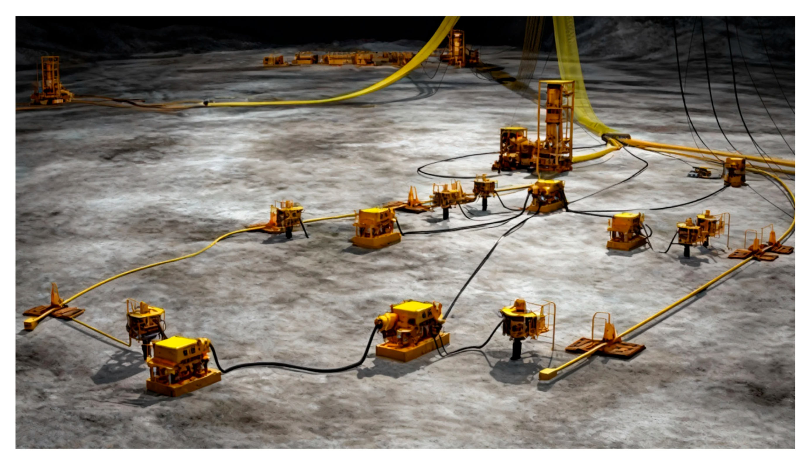Figure 1 illustrates a schematic layout of a deepwater oil and gas field based on a subsea production system.

Scholars have extensively researched optimization models and algorithms for subsea production system layouts. The evolution of these methods spans from classical techniques like Lagrange multipliers and derivative-based approaches to mathematical programming, including Linear Programming (LP) [5] and Nonlinear Programming (NLP) [6], and further to Mixed-Integer Nonlinear Programming (MINLP) for integrated layout optimization [7,8]. In 2012, Yingying Wang et al. [9]. developed an MINLP model for well-cluster partitioning to optimize manifold placement and wellhead connections. Subsequently, in 2014, they proposed an MINLP model for optimal cluster manifold layout based on Pipeline End Manifolds (PLEM) and implemented a dedicated algorithm in MATLAB 2020b, demonstrating the model’s effectiveness and providing quantitative guidance for engineering practice [10]. In 2016, Rodrigues et al. [11] introduced a generalized model to optimize offshore platform location, size, and well allocation, minimizing total platform and drilling costs while addressing complexities of water depth and well count.

In 2017, Ju YoungKang et al. [12] introduced the Laplacian smoothing algorithm to automatically optimize the smoothness of the pipeline path. Yuanlong Yue et al. [13,14] successively established optimization models integrating seabed terrain and obstacle constraints, aiming at reducing the total cost of control system layout or balancing multi-objective requirements. These studies provide effective methods for solving specific path optimization problems, but have not been comprehensively considered from the overall system architecture level.

In order to generate a better overall scheme, the research paradigm has gradually shifted from local optimization to automatic synthesis of system layouts. In 2018, Rosa et al. [15] proposed a practical and efficient method for the design of subsea production networks, considering the number of installed manifolds and platforms, location, well assignment to the collection system, and pipe diameter. In 2023, Philip Stape et al. [1] presented methodologies to automate the synthesis of subsea layouts for oil production systems, achieving a higher number of design alternatives in less time, with increased efficiency and a significant reduction in associated costs. Next year, Soban Babu Beemaraj et al. [16] presented a framework for early-stage layout design of subsea production systems, which decomposes the layout design problem into its four subsystem-level problems and is able to generate quick and feasible design options. However, its model accuracy and adaptability in dealing with specific engineering constraints still need to be strengthened. In 2023, Cheng Hong et al. [17] presented a Mixed-Integer Linear Programming (MILP) model for subsea power network layout optimization, incorporating capacity limits and obstacle avoidance to meet practical design requirements.

For solving such models, intelligent optimization algorithms are widely adopted to avoid local optima, accelerate convergence, and handle multi-objective constraints. Common methods include Genetic Algorithm (GA) [18], Particle Swarm Optimization (PSO) [19], and Simulated Annealing (SA). In 2018, Cheng Hong et al. [20] proposed a comprehensive optimization model for subsea layout design, minimizing total pipeline length through SA coupled with Dijkstra’s algorithm, effectively reducing pipeline installation costs and fluid transport losses. In 2020, Mohammed K. presents an integrated approach integrating the optimization of realistic drilling well paths, platform location, and well allocation using a combination of Constrained Optimization by Linear Approximation (COBYLA) and Mixed Integer Linear Programming (MILP) [21]. In 2023, Cheng Hong et al. [22] proposed a MINLP model. Through the model, the pipeline network topology structure, which reflects the allocations among the subsea wells, manifolds, and processing terminals, the routes of pipes, as well as the size of the facilities, could be figured out. In 2024, Yi Wang et al. [23] introduced an integrated mathematical model optimized via Modified Adaptive Particle Swarm Optimization (MAPSO), significantly reducing pipeline length and investment costs under seabed terrain constraints. Also in 2024, Wang J et al. [24] proposed a multi-ethnic ant colony parallel chaotic search method for 3D terrain path planning, leveraging parallel computing to balance energy consumption and distance while avoiding local optima.

Yingying Wang et al. (2012) [9] developed a mathematical model for well-to-cluster allocation to optimize cluster manifold layout, reducing subjectivity in empirical methods. Chen et al. (2017) [25] formulated a model for subsea well clustering in manifold layouts, focusing on connection-path optimization and cost reduction to provide quantitative references. Aparna (2019) [26] enhanced bipartite K-means with a Canonical Genetic Algorithm (CGA) to optimize cluster-center initialization, improving accuracy and stability. Wang et al. (2021) [27] developed algorithms based on complex iterative structures and unsupervised learning, taking into account bundle manifold layout scenarios, wellhead grouping, and intermanifold connection relationships. Beemaraj et al. (2024) [28] established a simulation framework integrating drilling-center clustering and manifold optimization, resolving well-clustering challenges in cluster manifold layouts; however, this method still has room for improvement in dealing with strict 3D terrain and global optimality.

In summary, current intelligent optimization algorithms for mathematical models predominantly use standard or modified PSO. While these offer fast convergence and global search capabilities, they remain prone to local optima and struggle with deep-sea complexities. Crucially, systematic studies on the impact of 3D terrain and obstacles are lacking. Therefore, this paper aims to solve the current research gap and proposes a multi-level integrated optimization model considering 3D terrain constraints. The core innovation of the model lies in the integrated modeling of seabed three-dimensional terrain, obstacle area, target location, pipeline routing, and manifold connection. To minimize the total investment cost, a strong nonlinear and multi-constraint overall optimization model is constructed, and an efficient solution algorithm is designed to realize the global optimal layout and provide more reliable decision support for deep-sea engineering practice.

2. Assumption

When designing a subsea production system layout, it is essential to comprehensively integrate systems engineering research across multiple specialized domains, including oil and gas field types, reservoir depth, hydrocarbon distribution, development strategies, drilling and completion methods, flow assurance, subsea pipelines, and types of subsea production facilities. Given the wide variety of equipment and complex influencing factors involved in subsea production systems, certain elements are appropriately simplified during model development to facilitate layout optimization while ensuring compliance with engineering requirements. This paper mainly focuses on the layout optimization during the terrain stabilization phase. Seafloor sedimentary change, stratigraphic slip, and subsurface uncertainty will be the important direction of model dynamic research in the future.

2.1. Reservoir Target

A reservoir target point refers to a specific location or area within an oil and gas reservoir determined based on subsurface geology, reservoir characteristics, and fluid distribution. In this study, the coordinate of the first entry point into the reservoir formation serves as the reservoir target point. These locations are typically selected as target zones for drilling operations or engineering activities such as stimulation and development, aiming to maximize hydrocarbon recovery efficiency.

Typically, reservoir target data provided in oil and gas engineering includes wellhead and target coordinates. One wellhead corresponds to one target zone, which contains multiple target coordinates. Each target zone is defined by two points: entry point, the starting position of the reservoir wellbore section; exit point, the endpoint of the reservoir wellbore section. To simplify drilling cost calculations, the first entry point into the reservoir formation is used as the target coordinate. Drilling costs are then computed based on the distance between this target point and the drilling center.

2.2. Configuration of Bottom

In marine surveying and seabed terrain modeling, the Digital Elevation Model (DEM) is commonly used to represent seabed topography. It digitally captures the three-dimensional morphology of the seabed through grid-point elevation values, exclusively containing natural terrain information.

The Raster Model is one of the most widely used methods for representing terrain elevation data within DEMs. It constructs a digital representation of terrain by dividing the surface into a regular two-dimensional grid (referred to as cells or grid cells) and storing an elevation value within each cell. The core characteristic of the raster model is its regular grid structure, which facilitates computer processing and spatial analysis.

The raster model is typically represented using a matrix or two-dimensional array, where each element corresponds to the elevation value of a grid cell. Mathematically, the raster model can be expressed as a matrix in the following form:

$$Z=\left[\begin{array}{ccc}{z}_{1,1}& \cdots & z_{1,n}\\ ⋮& \ddots & ⋮\\ z_{m,1}& \cdots & z_{m,n}\end{array}\right]$$

(1)

Here, $z_{i,j}$ represents the elevation value of the grid cell at row $i$ and column $j$, while m and n denote the total number of rows and columns in the raster DEM, respectively. Elevation values from raster map data can be read using Python V3.10.8’s GDAL library, where each value in the two-dimensional array corresponds to the average elevation of the terrain area represented by its respective grid cell.

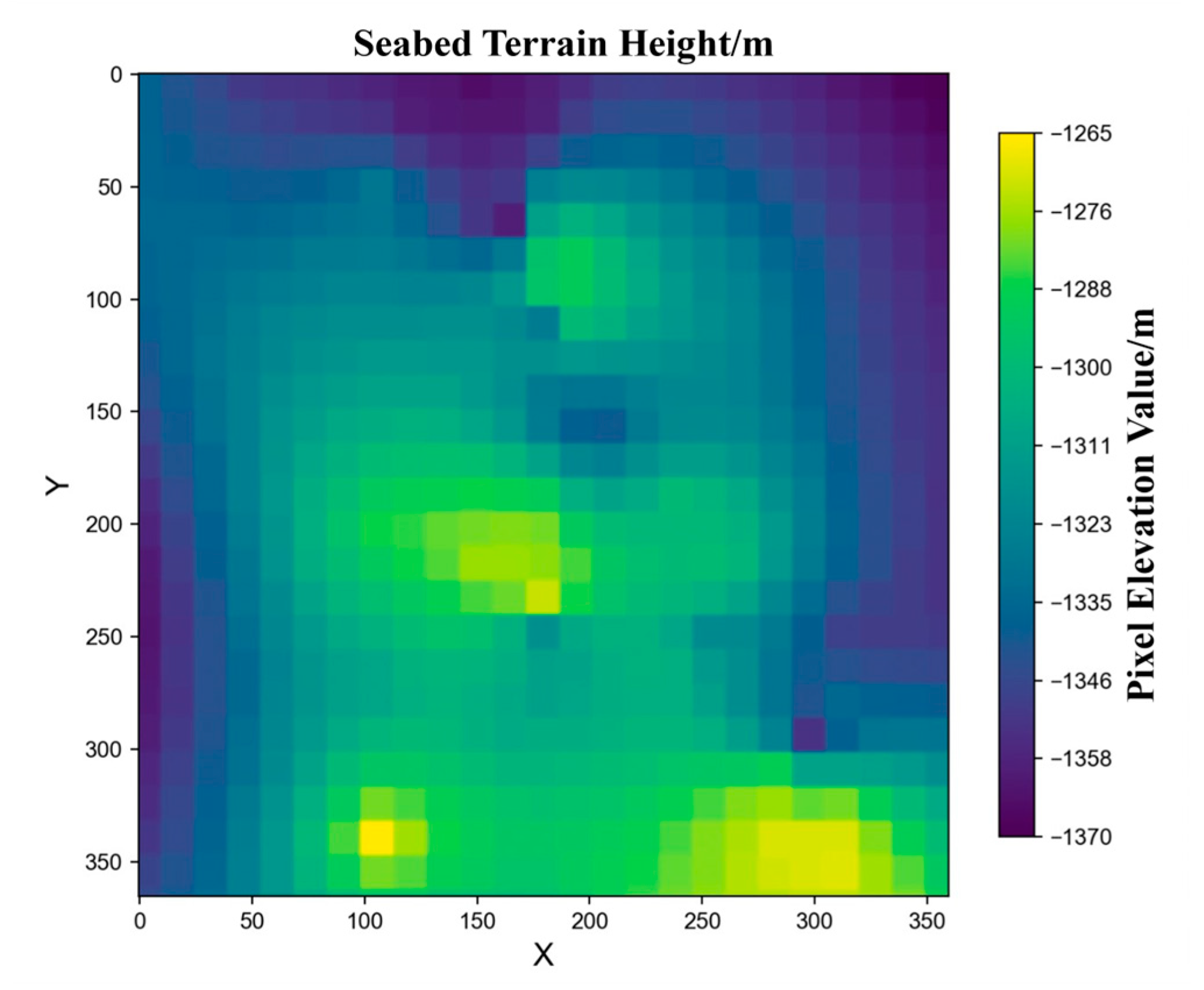
Raster resolution refers to the actual ground dimension represented by each grid cell, typically measured in meters (m). In this study, a $10 \mathrm{km}\times 10 \mathrm{km}$ seabed area in the South China Sea is used as an example, with a map resolution of 30 m. The raster terrain data contains $360\times 360$ data points and is stored in .tiff format. After reading the elevation data as a two-dimensional array from this raster terrain, a color-coded visualization is applied to represent elevation magnitudes across grid cells, as illustrated in Figure 2.

2.3. Seabed Obstacle

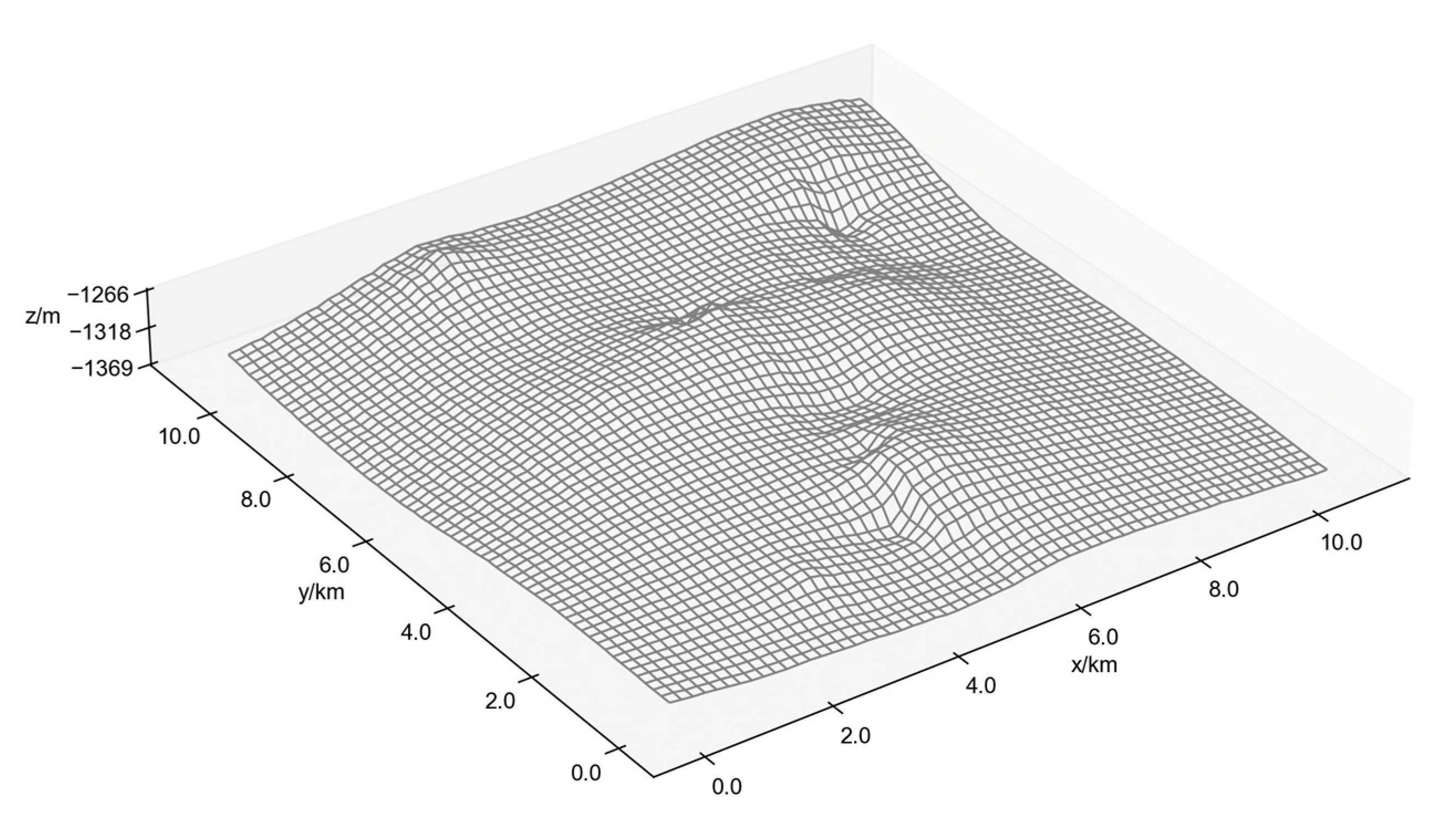
In practical seabed environments, complex topographical features such as ridges and trenches can significantly impact subsea equipment stability. To ensure safety while enhancing the scientific rigor and intelligence of layout designs, high-resolution DEM data must be employed for precise obstacle identification. Engineering practice faces challenges in mathematically describing irregular 3D obstacles, typically addressed through two approximation approaches: elementary function superposition and polygonal approximation (where precision improves with increased polygon edges). However, for highly complex and irregular obstacle zones, elementary function superposition often fails to achieve effective modeling, and traditional mathematical functions prove inadequate for direct description. Given these constraints, polygonal approximation has emerged as the primary method for characterizing such complex obstacle areas due to its operational flexibility and feasibility. Seabed elevation data are derived from actual South China Sea DEM measurements and assume that topographic relief within ±5 m does not affect path feasibility, and we assume that no geological and seabed topography changes occur during the subsea layout. Representative seabed obstacles are illustrated in Figure 3.

3. Layout Optimization Model Construction

3.1. Reservoir Target Grouping Optimization Model

3.1.1. Target Grouping Problem Description

Optimizing drilling center placement is a critical aspect of subsea production system layout design, as it directly determines the number and location of cluster manifolds, drilling costs, and ultimately impacts the system’s total investment. While reservoir target points are fixed, adjusting drilling center layouts alters the horizontal displacement of targets, thereby influencing drilling depth and expenses.

This study establishes a total investment optimization model incorporating manifold and drilling costs, with the objective of minimizing the sum of Euclidean distances between target points and drilling centers. This approach is based on the proportional relationship between horizontal projection distances of targets to drilling centers.

The reservoir target grouping optimization problem encompasses three key issues:

(1) Number of drilling centers;

(2) Assignment relationships between drilling centers and target points;

(3) Positions of drilling centers (which also represent cluster manifold locations).

Key modeling assumptions: A one-to-one correspondence exists between the first reservoir entry point and the wellhead. Drilling center positions obtained through target grouping optimization serve as cluster manifold locations. Target points assigned to a drilling center correspond to wellheads connected to that manifold. Implementation workflow: (1) After determining drilling center positions (manifold locations), install manifolds at these sites. (2) Arrange wellheads within a 30–50 m radius around each manifold, matching the number of associated reservoir targets. (3) Connect manifolds to wellheads using jumpers.

Given the fixed one-to-one relationship between wellheads and target points, the manifold-wellhead connection cost can be treated as a distance-dependent constant.

3.1.2. Target Grouping Constraints

Given a reservoir target dataset containing $n$ targets $T_i$ with coordinates $\left(x_i,y_i,z_i,\right)$, where $i=1,2,\dots ,n$, a clustering algorithm is applied to partition these targets into $m$ groups based on their coordinates. The geometric centroid of each target group defines the manifold location. Each manifold corresponds to one target group, with manifold positions denoted as $M_j$ ($j=1,2,\dots ,m$). The manifold position $M_j$ is calculated using Equation (2):

$$M_j={{\displaystyle \sum }}_{k=1}^{k_j}{\displaystyle \frac{T_{j,k}}{k_j}}$$

(2)

where $T_{j,k}$ represents the kth reservoir target coordinate of group J, $k_j$ is the number of targets contained in group j, and $M_j$ is the geometric center of group j targets.

The feasible number of manifolds m is constrained by the wellhead count and the slot capacity limits of cluster manifolds. The slot capacity must be an even number, with options restricted to 2, 4, 6, 8, or 10 slots per manifold. Defining $W_{min}=2$ (minimum slots) and $W_{max}=10$ (maximum slots), the allowable range for the number of manifolds m is determined by its minimum $M_{\min }$ and maximum $M_{\max }$ values. Here, n is the total number of reservoir targets. Equation (5) specifies the constraint for m:

$$M_{min}={\displaystyle \frac{n}{W_{max}}}$$

(3)

$$M_{max}={\displaystyle \frac{n}{W_{min}}}$$

(4)

$$M_{min}\le m\le M_{max}$$

(5)

Since wellbore trajectories are not considered, the drilling cost between a drilling center and a reservoir target is calculated based on their horizontal distance, denoted as $c_d$ (unit: 10,000 RMB/m). After determining the drilling center position, this location serves as the installation site for the manifold. Wellheads are then arranged within a 30–50 m radius around each manifold, matching the number of associated reservoir targets. Manifolds and wellheads are connected via jumpers.

To obtain an optimal reservoir target grouping solution, constraints must be established to align with engineering requirements. The constraints for reservoir target grouping are defined as follows:

(1) Each reservoir target is exclusively assigned to one wellhead and connects to only one manifold. The connection relationship between manifold $M_j$ and reservoir target $i$ is defined by a binary variable $x_{ij}$, where $x_{ij}=1$ indicates that target $i$ is assigned to manifold $M_j$, and $x_{ij}=0$ indicates no assignment. Therefore, a connection relationship matrix between the manifold and the target is formed as $X={(x_{ij})}_{m\times n}$. The constraints of the connection between the target and the manifold are expressed as follows:

$${{\displaystyle \sum }}_{j=1}^m{x}_{ij}=x_{i1}+x_{i2}+\dots +x_{im}=1,i=1,2,\dots ,n$$

(6)

(2) The number of wellheads connected to each manifold must not exceed the manifold’s slot capacity. The sum of each column in the connection matrix $X$ represents the number of wellheads connected to a manifold, and the slot capacity $W_{sj}$ must be an even integer selected from the predefined options.

(3) The Euclidean distance from each manifold position $M_j$ to its connected target level does not exceed Lmax. The constraint is expressed as follows:

$$‖T_{j,k}-M_j‖\le L_{max}$$

(7)

3.1.3. Target Grouping Optimization Objective Function

Subsea wellheads associated with reservoir targets are typically interconnected via gathering facilities, such as manifolds, PLEMs (Pipeline End Manifolds), PLETs (Pipeline End Terminations), jumpers, and subsea connection systems, while also being optimally linked to floating platforms through subsea export pipelines. Given the coordinates of reservoir targets, the optimization process involves partitioning targets into groups, determining the grouping scheme that minimizes connection costs between targets and manifolds while satisfying all constraints, and establishing manifold positions, quantities, and slot configurations to finalize the manifold layout.

The target grouping optimization aims to minimize total drilling and production costs, expressed through the objective function:

$$C_{well}={{\displaystyle \sum }}_{j=1}^m{\displaystyle \sum }_{k=1}^{k_i}‖T_{j,k}-M_j‖\cdot c_d$$

(8)

The manufacturing cost $C_m$ of each group of manifold equipment is expressed as follows:

$$C_m={{\displaystyle \sum }}_{j=1}^m{C}_m^k,k\in \left\{2,4,6,8,10\right\}$$

(9)

The overall drilling cost of reservoir target grouping optimization is expressed as $C_{drill}$, which is expressed as follows:

$$\min C_{drill}=C_{well}+C_m$$

(10)

where $‖T_{j,k}-M_j‖$ is the Euclidean distance from the $k$th reservoir target $T_{j,k}$ of the $j$th group to the horizontal plane of the $j$th group manifold $M_j$; the cost of connecting the target to the manifold is $c_d$, ten thousand yuan/m; $C_m^k$ is the manufacturing cost of manifold equipment containing $k$ well slots, with a unit of ten thousand yuan.

3.2. Pipeline Path Planning Model Under Three-Dimensional Seabed Terrain

3.2.1. Construction of Three-Dimensional Seabed Terrain Surface

Prepare data for the seabed Digital Elevation Model (DEM). The seabed DEM stores terrain data in raster format, where each pixel contains a depth or elevation value. Acquire the DEM data for the seabed area relevant to the reservoir engineering project.

Seabed topography and target data are sourced from DEM data and reservoir coordinates of the public survey area of Block A in the South China Sea (CNODC-2023 survey line), with a resolution of 30 m × 30 m [29]. By reading the terrain DEM data and performing 3D terrain visualization, the constructed surface model based on the raster representation is depicted in Figure 4.

3.2.2. Pipeline Path Objective Function

When constructing a three-dimensional seabed terrain based on digital elevation model (DEM) data, if two points are both located in passable regions (not within obstacle areas), we typically aim to obtain the shortest path along the terrain surface between them and its length.

First, convert the DEM raster into a discrete graph. Each center point $(i,j)$ of a DEM raster is transformed into a node $v_{i,j}$ in the graph, with attributes including planar coordinates $\left(x_i,y_j\right)$ and an elevation value $z_{i,j}$. When the horizontal and vertical spacing of the raster are, respectively, $\Delta x$ and $\Delta y$ (usually set to be equal, denoted as $\Delta =\Delta x=\Delta y$), where Δ represents the resolution of the raster terrain, the planar coordinates $\left(x_i,y_j\right)$ are calculated as $x_i=i\cdot \Delta$⋅Δ and $y_i=j\cdot \Delta$. The three-dimensional coordinates of the node are $\left(x_i,y_j,z_{i,j}\right)$. In regular rasters, edges are constructed between nodes. There are three edge connection methods for nodes: 4-adjacency, 8-adjacency, and 16-adjacency, and schematics of these three adjacency methods are shown in Figure 5.

Four-adjacency considers only the direct connections between a grid node and its up, down, left, and right neighbors. Movement along diagonal directions is prohibited, resulting in staircase-like paths that are longer than actual routes and exhibit poor path approximation.

Eight-adjacency extends this by including connections to four diagonal neighbors in addition to the four cardinal directions. This yields smoother paths without pronounced stair-stepping, closely approximating the true shortest path.

Sixteen-adjacency further incorporates second-nearest neighbors beyond eight-adjacency connections. While it achieves even closer approximations to the true shortest path, the significant increase in edges reduces graph search efficiency.

Given that eight-adjacency optimally balances path accuracy and computational efficiency, this study adopts it as the path-search model.

For any two adjacent nodes $v_{i,j}$ and $v_{k,l}$, their Euclidean distances on the three-dimensional terrain surface are as follows:

$$w\left(v_{i,j},v_{k,l}\right)=\sqrt{\Delta x^2++\Delta y^2+\Delta z^2}$$

(11)

where $\Delta x=\left(x_k-x_i\right)$ is the horizontal distance, $\Delta y=\left(y_l-y_j\right)$ is the vertical distance, and $\Delta z=\left(z_{k,l}-z_{i,j}\right)$ is the elevation difference between two points.

Due to the grid spacing $\Delta =\Delta x=\Delta y$, the horizontal or vertical edge distance is calculated as follows:

$$w\left(v_{i,j},v_{i+1,j}\right)=\sqrt{{\Delta }^2+\Delta z^2}$$

(12)

The side length in the diagonal direction is calculated as follows:

$$w\left(v_{i,j},v_{i+1,j+1}\right)=\sqrt{2{\Delta }^2+\Delta z^2}$$

(13)

Assume the start point is $v_{start}=\left(i_0,j_0\right)$ and the endpoint is $v_{end}=\left(i_n,j_n\right)$. The path $V$ from the start point to the end point is a sequence of nodes $V=\left\{v_{i_0{j}_0},v_{i_1{j}_1},\dots ,v_{i_n{j}_n}\right\}$. The total distance of the starting path of the path node from the submarine pipeline $v_{start}$ to the destination $v_{end}$ is the sum of the distances of all nodes along the path, which is expressed as follows:

$$L\left(V\right)={\displaystyle \sum }_{k=0}^{n-1}w(v_{i_k{j}_k},v_{i_{k+1}{j}_{k+1}})$$

(14)

The objective of the shortest path problem is to find the path $L\left(V\right)$ from $v_{start}$ to $v_{end}$ such that the total distance $L\left(V\right)$ is minimized. The objective function for calculating the shortest pipeline path between two points in a 3D seabed terrain is expressed as follows:

$$V=\underset{\mathrm{v}}{\mathrm{argmin}}{{\displaystyle \sum }}_{k=0}^{n-1}w\left(v_{i_k{j}_k},v_{i_{k+1}{j}_{k+1}}\right)$$

(15)

4. Four Target Grouping Optimization Algorithms and Solutions

K-means and its improved algorithms have the characteristics of high computational efficiency, stable convergence, and suitability for clustering in continuous spaces. Moreover, when coupled with the integer linear programming model, they can directly express the objective of minimizing drilling costs. In contrast, density-based clustering and spectral clustering are sensitive to noise and sample density in high-dimensional spaces and are not suitable for constrained grouping problems.

4.1. K-Means Dynamic Clustering Algorithm

The K-means clustering algorithm is a classical unsupervised learning method designed to address clustering problems. Its core principle involves iteratively partitioning the reservoir target data into $m$ non-overlapping clusters to minimize the Within-Cluster Sum of Squared Errors (WCSS). This optimization ensures the sum of distances between data points and their cluster centroids is minimized, achieving effective data clustering.

Despite its widespread adoption, K-means exhibits inherent limitations: sensitivity to initial centroids, dependence on predefining the number of clusters $m$, and vulnerability to data distribution characteristics. Nevertheless, due to its computational efficiency, ease of implementation, and proven effectiveness in practical applications, K-means remains one of the most extensively utilized clustering algorithms across both industry and academia.

4.2. Bisecting K-Means Clustering Algorithm

Bisecting K-means is an improved version of K-means, specifically designed to address the issue of “the initial selection of centers in ordinary K-means being prone to becoming stuck in local optima”. It combines the ideas of “splitting clustering” and K-means: instead of dividing all the data into $m$ groups at once, it gradually “splits” the dataset step by step, ultimately obtaining m groups of reservoir target points. The purpose of this approach is to enhance the efficiency and effectiveness of clustering, especially suitable for scenarios with “extremely large data volumes” or “high data dimensions”.

Unlike ordinary K-means, which directly and rigidly divides all data into K categories, bisecting K-means “gradually refines the groupings”. This reduces the risk of becoming stuck in local optima and makes the clustering results more stable. The ultimate goal of bisecting K-means is to minimize the sum of squared errors within each group. Compared to traditional K-means, it is faster when dealing with large-scale data and is less sensitive to the initial selection of centers. However, it also has limitations: the “splitting order” and “splitting strategy” during the grouping process can affect the outcome; if the data distribution is particularly uneven, additional optimization for specific problems is still required.

4.3. Target Grouping Method Based on Genetic Algorithm

The Genetic Algorithm (GA) is an optimization method inspired by natural selection and genetic principles. It emulates biological mechanisms, including inheritance, mutation, and selection, to iteratively converge toward optimal solutions. In this context, GA aims to determine optimal drilling center positions that minimize the sum of Euclidean distances between each target group’s centroid and its drilling center.

As a robust heuristic optimization technique, GA excels at solving complex nonlinear problems lacking analytical solutions or exhibiting irregular constraints. Its strengths include broad applicability and powerful global search capabilities. However, notable limitations persist, including high computational complexity, sensitivity to parameter tuning, and slow convergence rates.

4.4. K-Means-ILP Clustering Algorithm

Due to the problem constraints that the manifold location of each cluster must be the geometric center of its target points, and additional constraints requiring the number of target points in each group to not exceed $W_{max}$ and the distance from each target point to the geometric center of its group to not exceed $L_{max}$, a clustering algorithm with capacity and radius constraints can be adopted. A feasible heuristic algorithm is designed as follows:

Step 1. Initialize the data by treating all target points as a single initial cluster, i.e., the initial number of groups is 1.

Step 2. Repeat the following steps until the number of clusters reaches $m$.

Select the target cluster to be split: Select the group with the largest sum of squared errors in the cluster from all the existing groups (preferentially splitting the group with ‘large internal differences’ can reduce the error of the overall clustering faster); using the ‘binary K-means algorithm’, the selected groups are split into two sub-groups, ensuring that each subcluster contains no more than $W_{max}$ target points.

Assume the two resulting clusters collectively contain $n$ target points. Since the number of target points in these two groups satisfies the constraints, re-partitioning them into two groups using an ILP method is guaranteed to yield a feasible solution. The solution approach for ILP is as follows:

$$\underset{x}{\min }{f}^{\prime }x$$

(16)

$$\mathrm{s}.\mathrm{t}. \left\{\begin{array}{c}Ax\le b\\ Bx=c\\ x_{ij}\in \left\{0,1\right\}\end{array}\right.$$

(17)

where $f={\left[f_{1,1},f_{2,1},\dots ,f_{n,1},f_{1,2},f_{2,2},\dots ,f_{n,2}\right]}^{\prime }\in R^{2n}$, and $f_{i,j}$ denotes the distance between the $i$th target point and the geometric center of the $j$th group. $x={\left[x_{1,1},x_{2,1},\dots ,x_{n,1},x_{1,2},x_{2,2},\dots ,x_{n,2}\right]}^{\prime }\in R^{2n}$, where the objective function represents the sum of distances from target points to the geometric center of their respective groups.

$$A=\left[\begin{array}{cccccccc}1& 1& \cdots & 1& 0& 0& \cdots & 0\\ 0& 0& \cdots & 0& 1& 1& \cdots & 1\end{array}\right]\in R^{2\times 2n}, b=\left[\begin{array}{c}{b}_0\\ b_0\end{array}\right]$$

(18)

The matrix $A$ has all elements equal to 1 in the first $n$ columns of the first row and the last $n$ columns of the second row, and all other elements equal to 0. $b_0$ represents the maximum number of well slots in the manifold $W_{max}$, which is also the maximum number of target points allowed in each cluster. The constraint condition $x\le b$ indicates that after dividing $n$ oil reservoir target points into two groups, and the number of target points in each group does not exceed $b_0$ (i.e.,$W_{max}$).

$$B=\left[\begin{array}{cc}\begin{array}{ccc}1& \cdots & 0\\ ⋮& \ddots & ⋮\\ 0& \cdots & 1\end{array}& \begin{array}{ccc}1& \cdots & 0\\ ⋮& \ddots & ⋮\\ 0& \cdots & 1\end{array}\end{array}\right]\in R^{n\times 2n}, c=\left[\begin{array}{c}1\\ ⋮\\ 1\end{array}\right]\in R^n$$

(19)

where the first $n$ columns and the last $n$ columns of the matrix $B$ form an $n$-order identity matrix, and the constraint condition $x=c$ indicates that each oil reservoir target can only belong to one of the groups.

The target partitioning problem is initially solved by the bipartite K-means algorithm to obtain an initial feasible solution $x_0$. Subsequently, the linear programming module in the SciPy library is invoked to solve the above ILP problem and obtain the optimal solution $x$, thereby deriving the optimal grouping scheme for re-dividing the original two groups.

Update the cluster set: Replace the original clusters with the two sub-clusters obtained from linear programming, increasing the total number of clusters by one.

Step 3. Termination condition: When the number of clusters reaches $m$, the algorithm terminates, yielding the final grouping of $m$ manifolds for oil reservoir targets.

Step 4. Verification: Check whether the distance from each target to the geometric center of its group exceeds $L_{max}$. If any target exceeds $L_{max}$, the clustering into $m$ groups fails; otherwise, the partitioning into $m$ groups is successful, and the targets and manifold positions of the $m$ groups are returned.

The heuristic clustering algorithm module rapidly generates an initial solution satisfying intra-cluster connection distance and capacity constraints through iterative assignment, centroid updating, and local adjustments. Subsequently, an Integer Linear Programming (ILP) model refines local regions within this heuristic solution by introducing binary variables to precisely capture equipment assignment and type selection decisions, thereby accurately accounting for piecewise equipment costs.

This hybrid algorithm alternately applies heuristic global search and ILP-based local refinement, achieving dual advantages, namely maintaining computational efficiency and enhancing solution quality. It proves particularly suitable for medium-scale reservoir target grouping problems with complex constraints. The hybrid strategy effectively balances solution time and global optimality, making it highly applicable to practical engineering challenges in target grouping and manifold placement.

4.5. Example Verification of Four Algorithms

Based on the four algorithms above, we take 36 target coordinates in a specific area of the South China Sea oilfield as an example (Figure 6). The water depth in this region ranges from 1200 m to 1500 m, and the seabed rectangular area measures approximately 10 km × 10 km. Since drilling costs are calculated based on the projected horizontal distance from each target to the drilling center (with a unit cost of CNY 50,000/m), the results of target grouping are visualized using 2D planar diagrams showing the connections between targets and drilling centers. This approach intuitively displays grouping outcomes and assigned drilling centers.

In this oilfield project, the manifold options range from 2 to 10 well slots. Therefore, the number of targets per cluster must not exceed the maximum well slots of the manifold $W_{max}=10$, and the distance from any target to its manifold must not exceed $W_{max}=6000 \mathrm{m}$. The input reservoir target coordinates are listed in

Table 1. Coordinates of submarine oil reservoir targets.

Reservoir Target	$\mathbf{Coordinate} (\mathbf{x},\mathbf{y},\mathbf{z})$	Reservoir Target	$\mathbf{Coordinate} (\mathbf{x},\mathbf{y},\mathbf{z})$
T1	(2484, 1431, −1331)	T19	(3964, 2650, −1315)
T2	(4566, 5700, −1333)	T20	(5422, 9333, −1331)
T3	(9013, 4839, −1305)	T21	(9416, 6722, −1297)
T4	(2125, 5856, −1301)	T22	(7869, 8642, −1330)
T5	(6775, 7319, −1301)	T23	(1545, 5889, −1320)
T6	(7846, 2746, −1310)	T24	(6737, 2387, −1306)
T7	(5553, 7500, −1302)	T25	(8088, 6279, −1306)
T8	(3664, 8360, −1325)	T26	(9087, 5473, −1302)
T9	(4011, 6634, −1324)	T27	(1137, 2961, −1342)
T10	(3717, 8814, −1332)	T28	(9126, 8866, −1304)
T11	(5392, 2055, −1313)	T29	(8249, 1948, −1322)
T12	(8321, 8659, −1330)	T30	(4673, 9030, −1332)
T13	(9366, 6062, −1300)	T31	(2949, 6076, −1291)
T14	(5752, 7097, −1301)	T32	(1814, 7692, −1327)
T15	(4209, 7074, −1322)	T33	(4037, 7472, −1321)
T16	(5592, 1759, −1315)	T34	(5876, 8024, −1304)
T17	(4178, 9235, −1336)	T35	(597, 2798, −1352)
T18	(8969, 4435, −1303)	T36	(1635, 4091, −1347)

, and manifold costs are detailed in

Table 2. Manifold cost table.

Type of Manifold	2 Well Slots	4 Well Slots	6 Well Slots	8 Well Slots	10 Well Slots
Cost/million yuan	1680	2400	3120	3600	4800

.

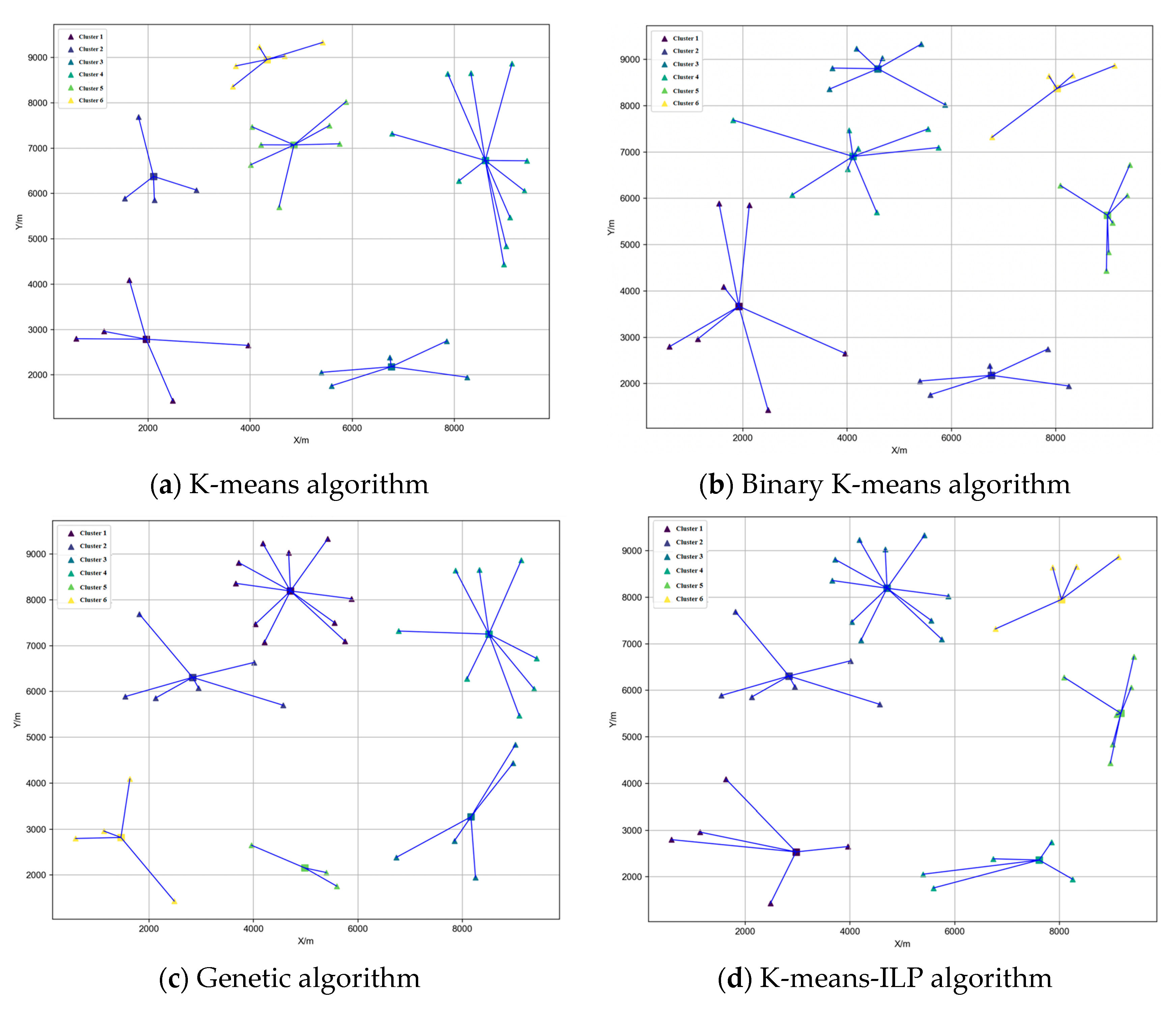
To compare four algorithms—K-means algorithm, bisecting K-means algorithm, genetic algorithm, and hybrid grouping optimization algorithm based on bisecting K-means and ILP—the following parameter settings were applied: for K-means, number of clusters K = n/8 and maximum iteration count = 100; for GA, population size = 50, crossover probability = 0.8, and mutation probability = 0.05; for the K-means-ILP model, tolerance ε = 10⁻³; for convergence criterion, rate of change in the objective function between adjacent generations was <0.001. Target data and constraints were substituted into the algorithms, with the number of manifolds (or drilling centers) m = 6. (The hyperparameters (such as the number of clusters and weight coefficients a, b, a₁, b₁) of the algorithm are determined by several rounds of preliminary tests, and their selection follows the principle of balance between convergence speed and stability). All algorithms were executed under identical hardware and computational resources. The results are presented in Figure 7 and

Table 3. Grouping results of four algorithms with a manifold of 6.

Algorithm	WCSS/m	Drilling Cost/Ten Thousand Yuan	Total Cost/Ten Thousand Yuan
K-means	46,072.44	230,362.21	249,322.21
Binary K-means	44,695.09	223,475.43	242,915.43
Genetic algorithm	42,708.57	213,542.85	232,022.85
K-means-ILP	41,640.09	208,200.45	227,160.45

.

Based on the clustering results of the four algorithms in the above table, the following conclusions can be drawn:

(1) The within-cluster sum of squared errors (WCSS) is positively proportional to drilling costs. The larger the sum of distances from targets to their assigned manifolds, the higher the drilling cost and the total optimization cost of target grouping. Therefore, the primary objective of reservoir target grouping optimization lies in minimizing WCSS.

(2) Judging from WCSS and total cost, the K-means-ILP algorithm performs the best, followed by the genetic algorithm and bisecting K-means. The K-means algorithm yields the largest WCSS, and its grouping stability is comparatively poor, being more sensitive to initial data points.

4.6. Comparative Analysis of Grouping Optimization Algorithms

To further verify the performance of the four algorithms, the results of reservoir target grouping under different manifold quantities when calculating the manifold quantity $m=5,6,\dots ,12$ for the reservoir targets are compared, as shown in Figure 8, which depicts the WCSS (within-cluster sum of squared errors) comparison of the four algorithms.

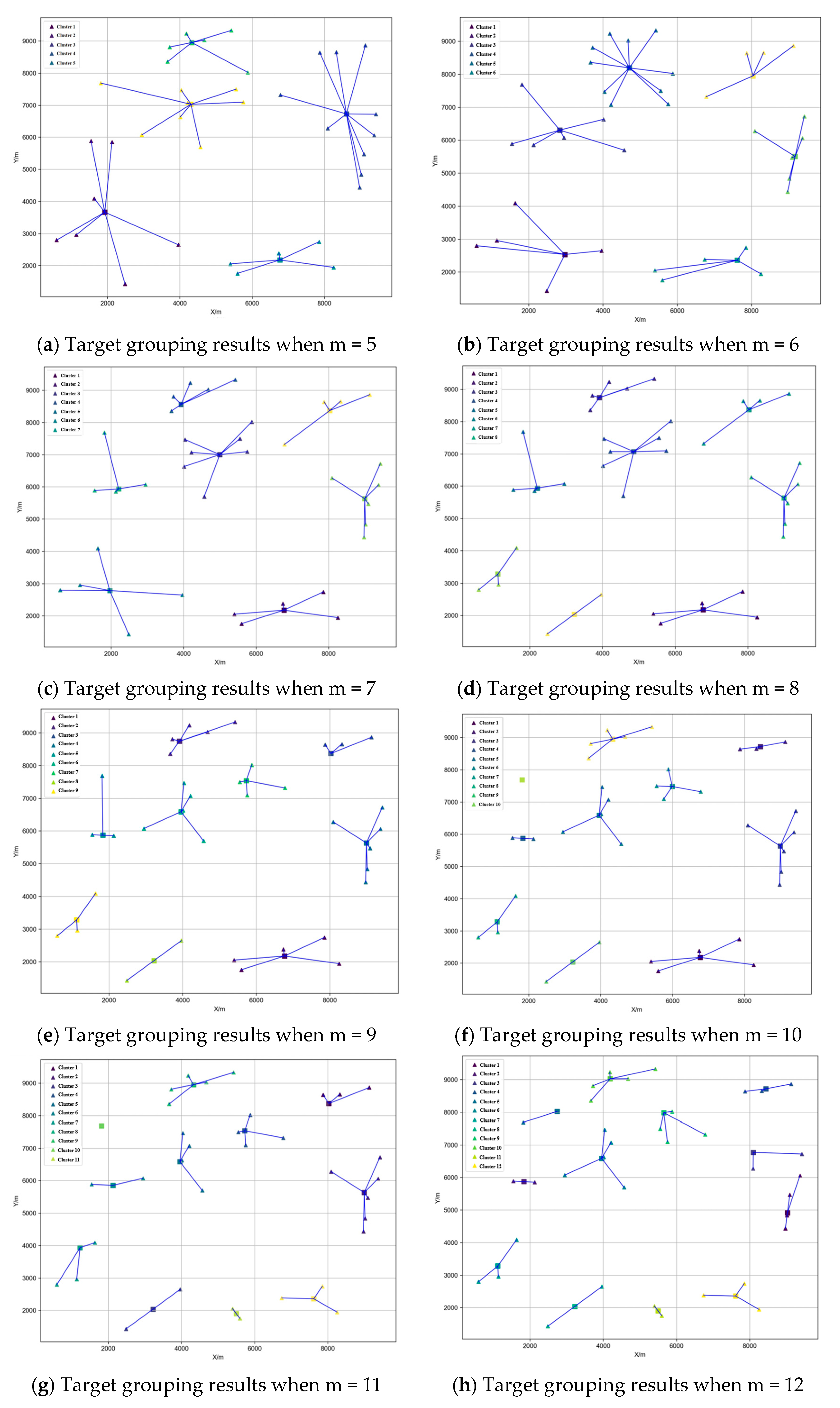
As shown in Figure 8, the K-means-ILP algorithm yields the smallest within-cluster sum of squared errors (WCSS) across different manifold quantities. This indicates that the K-means-ILP algorithm achieves the optimal grouping effect, outperforming the bisecting K-means algorithm, genetic algorithm, and conventional K-means algorithm. Subsequently, substituting manifold quantities $m=5,6,\dots ,12$ into the K-means-ILP algorithm, the corresponding grouping results are presented in Figure 9.

As shown in Figure 10, as the number of groups increases, the overall within-cluster sum of squares (WCSS) becomes significantly smaller. This trend of grouping results leads to an extreme scenario that does not align with engineering practicality, where placing a manifold at each target point causes the drilling cost to approach zero. In actual engineering scenarios, the installation and maintenance costs of manifolds must be considered. Moreover, connecting manifolds to each other, manifolds to PLEMs, and manifolds to FPSOs would significantly increase pipeline costs. Therefore, the local optimum of the subproblem does not satisfy the optimal solution for the overall layout, necessitating a holistic optimization approach for the subsea production system.

5. Layout Optimization Model Construction

5.1. The Digital Elevation Model Transformed into a Graph

The digital elevation model is a raster data structure. It is usually necessary to model the digital elevation model DEM as a graph data structure to effectively represent the spatial topological relationship of terrain data and support graph-based spatial calculation and optimization. In this model, the environment is discretized into regular grid cells, and each cell contains specific terrain information. In order to carry out efficient path planning, it is usually necessary to convert the grid model into a weighted graph so that the graph search algorithm can be used to calculate the optimal path.

The conversion of DEM rasters to graph structures is achieved by mapping each raster cell to a graph node and constructing topological connections based on eight-neighborhood relationships. Edge weights are dynamically defined according to application scenarios: horizontal distance weights only calculate planar Euclidean distances, suitable for flat terrain; elevation difference weights use the elevation difference Δh between adjacent cells to reflect the impact of terrain undulations. This conversion process requires a precise definition of neighborhood scope and weighting mechanisms to ensure the graph structure fully captures the spatial connectivity and elevation difference characteristics of the terrain. The constructed graph data structure can adopt different storage methods to accommodate various computational needs.

In practical DEM data processing, additional considerations include boundary issues and outlier handling. For boundary issues, cells at the edges of the DEM have incomplete neighborhoods, so invalid adjacency relationships must be removed during graph construction to ensure all edges lie within valid regions. For outlier handling, when elevation data is missing or anomalous, interpolation methods can be used to fill gaps, or these nodes can be ignored during graph construction to avoid affecting computational results. Through the above steps, a DEM can be converted into a graph data structure using eight-neighborhood relationships. The key to this process lies in accurately defining neighborhood scope, reasonably setting edge weights, and properly handling boundaries and missing values, ensuring the graph structure authentically and effectively represents the spatial connectivity and elevation difference characteristics of the terrain.

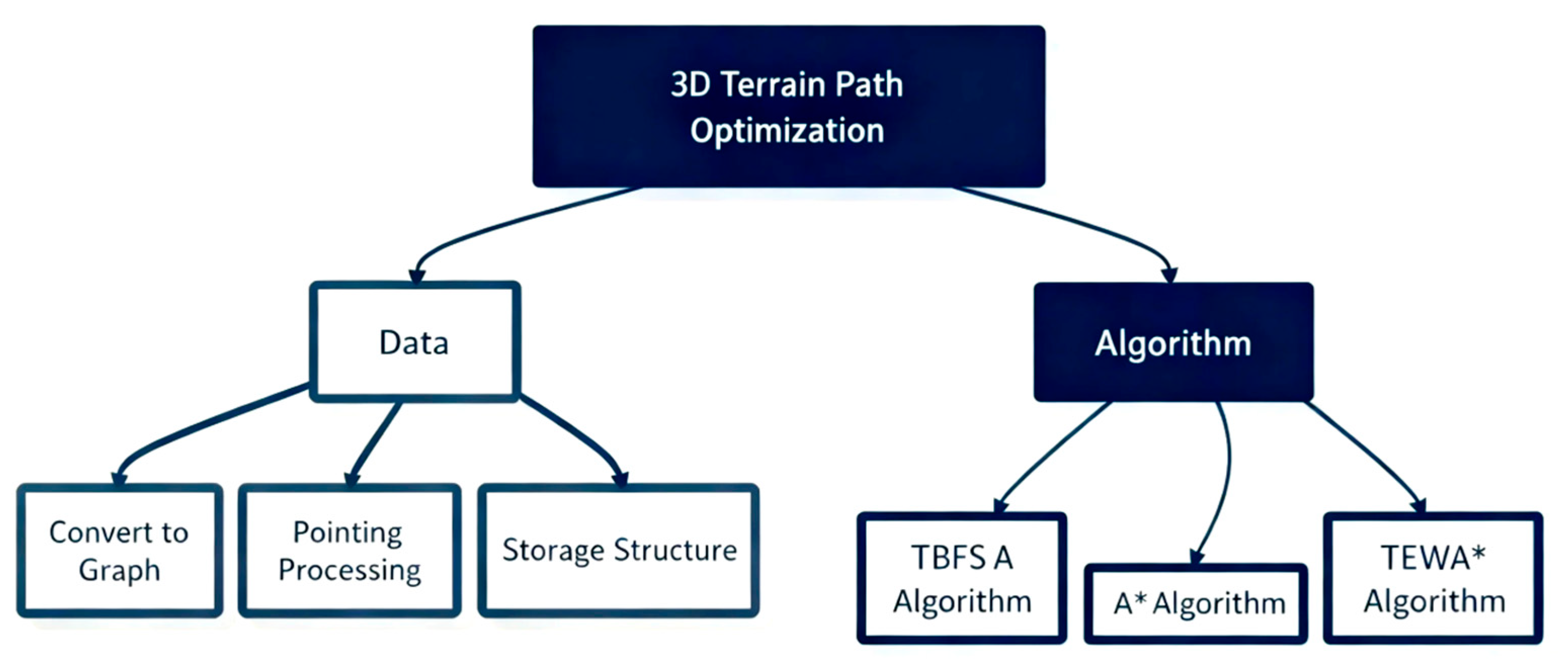
In the process of transforming DEM into a graph data structure with eight-neighborhood relationships, a data foundation is provided for path planning algorithm research. DEM path planning requires first converting the DEM raster map into a graph stored in a 2D array, then expanding search directions using 4-neighborhood, 8-neighborhood, or 16-neighborhood rules, and finally applying path planning algorithms to search for paths. The algorithm framework is shown in Figure 11.

5.2. Dijkstra Algorithm

Dijkstra’s algorithm is a classical shortest path algorithm, which is mainly used to calculate the shortest path from a single source point to all other vertices in a non-negative weight graph. Based on the greedy idea, the algorithm gradually expands the vertices with the shortest known path and finally ensures to find the global optimal solution. The Dijkstra algorithm is suitable for graphs with non-negative weights, which can guarantee the optimal solution. In the case of using ordinary array storage distance, the computational complexity is high $O\left(V^2\right)$, but the priority queue can be optimized to $O\left(E+VlogV\right)$, where the number of vertices $V$, the number of edges $E$, the expansion efficiency is lower than that of the heuristic method.

5.3. Directional Breadth-First Path Search Algorithm

On the basis of the breadth-first search algorithm, the two-way breadth-first search algorithm (TBFS) is developed. Its core idea is to perform breadth-first search (BFS) from both source and target points at the same time, and meet in the middle area of the search, thereby reducing the overall traversal scale. Compared with the traditional one-way BFS, TBFS has a significant time efficiency advantage in large-scale graphs.

TBFS effectively compresses the search space by initiating breadth-first search from both source and target points, which is suitable for quickly determining the connectivity and shortest path between two points in a large-scale graph. When the size of the graph increases, and the distance between the source point and the target point is far, the acceleration effect is particularly obvious compared to the one-way BFS.

5.4. Eight Neighborhood A* Algorithm

The eight-neighborhood A* algorithm (A-star algorithm) is a graph search algorithm based on heuristic search. Each node in the DEM grid map can expand in eight adjacent directions, which is mainly used to find the optimal path from the starting point to the target point in the weighted graph. It combines the advantages of the shortest path search strategy of the Dijkstra algorithm and the heuristic search of greedy best-first search. By comprehensively considering the known cost and estimated cost of the path, it can efficiently find the global optimal path in the solution space.

The core idea of the A* algorithm is to introduce a heuristic estimation function in the search process to more effectively guide the search to the target direction. Its evaluation function is defined as follows:

$$f\left(n\right)=g\left(n\right)+h\left(n\right)$$

(20)

Among them, $f\left(n\right)$ represents the combined cost estimate of the current node $n$; $g\left(n\right)$ represents the actual path cost (cumulative cost) from the start node $s$ to the current node $n$; $h\left(n\right)$ represents the heuristic estimate cost from the current node $n$ to the target node $t$ (i.e., the predicted minimum remaining cost). When $h\left(n\right)=0$, it reduces to Dijkstra’s algorithm.

During the search process, the A* algorithm consistently prioritizes expanding the node with the smallest $f\left(n\right)$ value, thereby accelerating search efficiency while guaranteeing the discovery of an optimal path. Its key advantage lies in its ability to perform efficient searches and identify a globally optimal solution. However, a notable limitation is its potentially high computational overhead in high-dimensional spaces or complex environments.

5.5. Terrain Enhanced Weighted A* Algorithm

In the traditional A* algorithm, heuristic functions generally use Euclidean distance or Manhattan distance. However, it is difficult to accurately reflect the cost of real terrain only by looking at the horizontal distance. For example, the slope of the terrain costs extra money to lay the pipeline, and the distribution of obstacles in complex terrain also affects the cost.

To this end, we introduce the concept of terrain cost, make corresponding improvements in the state expansion and evaluation function, and propose a Terrain Enhancement Weighted A* (TEWA*) path planning algorithm to achieve the shortest pipeline path planning in three-dimensional terrain.

Assume the elevation data is $Z\left[i\right]\left[j\right]$, and certain grids are known as non-passable areas (obstacles) or higher-cost areas. The planning goal is to find a path with the minimum cumulative cost from the start point $s$ to the endpoint $t$ on the Digital Elevation Model (DEM). The improvement of the TEWA* algorithm lies in the following steps.

1. State representation: The current node $n$ not only includes the 2D coordinates $\left(i,j\right)$ but also optionally incorporates elevation information or directly references $Z\left[i\right]\left[j\right]$.

2. The calculation of the actual cost $g\left(n\right)$:

$$g\left(n_{neighbor}\right)=g\left(n\right)+cost\left(n,n_{neighbor}\right)$$

(21)

where $cost\left(n,n_{neighbor}\right)$ consists of the factors including horizontal or vertical distance: in the 8-neighborhood context, the distance $\sqrt{\Delta x^2+\Delta y^2+\Delta z^2}$ can be adopted; elevation difference: a certain energy consumption or cost is assigned based on $\left|Z\left[i_1\right]\left[j_1\right]-Z\left[i_2\right]\left[j_2\right]\right|$$\left|Z\left[i_1\right]\left[j_1\right]-Z\left[i_2\right]\left[j_2\right]\right|$; obstacle penalty: if the adjacent grid is an obstacle, or is itself a high-cost area (such as mountain), the cost of this section of the road has to be extra high. The combination can be expressed as:

$$cost\left(n,n_{neighbor}\right)=\alpha \cdot d+\beta \cdot ObstacleFactor$$

(22)

where $d$ represents the horizontal distance between adjacent grid nodes, $\alpha ,\beta$ are the weighting coefficients for different factors, and $\mathrm{ObstacleFactor}$ denotes the additional cost for obstacles or surfaces with different traversal difficulties.

3. Improvement of heuristic function $h\left(n\right)$:

Traditional A* algorithm’s commonly used Euclidean distance or Manhattan distance can no longer effectively reflect terrain undulations. Therefore, terrain differences can be introduced as follows:

$$h\left(n\right)=\alpha 1\cdot H\left(n,t\right)+\beta 1\cdot V\left(n,t\right)$$

(23)

Among them, $H\left(n,t\right)$ represents the Euclidean distance between the current node $n$ and the target node $t$; $V\left(n,t\right)$ refers to the absolute elevation difference between the current node and the target, which can also be replaced by a slope-based estimate; $\alpha 1,\beta 1$ are balancing parameters used to control the relative importance of horizontal distance and vertical elevation difference in the heuristic function.

The TEWA* algorithm can be better adapted for path planning on digital elevation models, primarily demonstrated by its comprehensive consideration of terrain slope, elevation difference, and obstacle information. By incorporating elevation and obstacle information into both the cost function and the heuristic function, the algorithm can ensure feasibility while being closer to the actual terrain environment, avoiding obstacle areas, as shown in Figure 12 for its flowchart.

5.6. Implementation and Analysis of Three-Dimensional Surface Path Obstacle Avoidance Planning Algorithm

5.6.1. Construction of Seabed Obstacles

In a Digital Elevation Model (DEM), methods for constructing obstacle zones typically involve identifying and marking obstacle regions based on terrain characteristics. DEM raster models store terrain elevation values in a matrix structure, with each cell representing the elevation of a surface point. In deep-water oil and gas field path planning, this model characterizes seabed topography and identifies obstacle locations using elevation information. Since natural terrain with an elevation of zero does not exist in deep-sea environments, engineering practices often assign a unified elevation value of zero to obstacle zones to mark impassable areas. Obstacle zones are defined using four primary methods:

1. Elevation Threshold Method: For hazardous terrains like steep slopes or seamounts, a critical elevation threshold is set. Raster cells exceeding this threshold are classified as obstacles.

2. Slope Analysis Method: Steep regions are identified by calculating elevation change rates between adjacent raster cells. Slope values are derived using the Sobel operator or direct elevation difference algorithms. Areas exceeding a safety threshold are flagged as obstacles.

3. Spatial Annotation Method: Human-made obstacles unrelated to elevation (e.g., pipelines, artificial structures) are delineated using GIS polygon coordinates or manual annotations to define precise spatial boundaries.

4. Special Value Tagging Method: Obstacle raster cells are directly assigned specific values in the DEM matrix or added to the CloseList of pathfinding algorithms, forcing them to be marked as “visited” to avoid traversal.

The method adopted in this study marks obstacle zones by adding their raster cell coordinates to the CloseList, preventing repeated visits.

Table 4. Obstacle area vertex coordinates.

Obstacle Zone Coordinates	Obstacle 1	Obstacle 2
lower left corner	(1800, 1200, −1319)	(3000, 3600, −1311)
top left corner	(3000, 1200, −1334)	(5400, 3600, −1322)
lower right corner	(1800, 2400, −1302)	(3000, 4800, −1293)
top right corner	(3000, 2400, −1309)	(5400, 4800, −1273)

lists the coordinates of these rectangular obstacle zones within the raster map.

After constructing the obstacle area, the path planning algorithm avoids passing through these areas. The Dijkstra algorithm, TBFS algorithm, A* algorithm, and TWEA* algorithm take into account the obstacle area, adjust the path, make the path bypass the obstacle as far as possible, and select the area that can be passed for calculation.

5.6.2. Example Verification of Path Planning Obstacle Avoidance Algorithm

In the three-dimensional seabed terrain shown in Figure 5, two rectangular obstacle areas are set to verify the algorithms, evaluating the obstacle avoidance effects of four algorithms in three-dimensional terrain path planning. Taking a raster terrain map with dimensions of $10 \mathrm{km}\times 10 \mathrm{km}$ grid cells as an example (totaling $360\times 360$ data points and 129,600 grid units), with a map resolution of 30 m, path planning and obstacle avoidance verification are conducted for all four algorithms in this raster terrain environment. The 3D coordinates of the start point are (1080, 540, −1339), and of the end point are (10,020, 9000, −1271). The obstacle avoidance path planning results of the four algorithms are shown in Figure 13.

The path planning method based on digital raster maps, at its core, seeks the optimal route through the expansion of adjacent nodes. As the system expands outward from the current position, multiple adjacent cells appear around each node as candidate path points. The number of candidate points directly affects the performance of the algorithm: when there are more candidate points, the system requires more computing time but can generate smoother paths; when there are fewer candidate points, the calculation speed is faster, but the path may not be as refined. In all four algorithm examples, the node expansion method adopts an eight-neighborhood model with a step size of one. As clearly shown in Figure 13, although the path planning principles of the four algorithms all originate from node traversal search and can be used for obstacle avoidance and feasible path finding, they differ in terms of operational efficiency, path quality, and implementation complexity.

5.6.3. Comparative Analysis of Four Algorithms

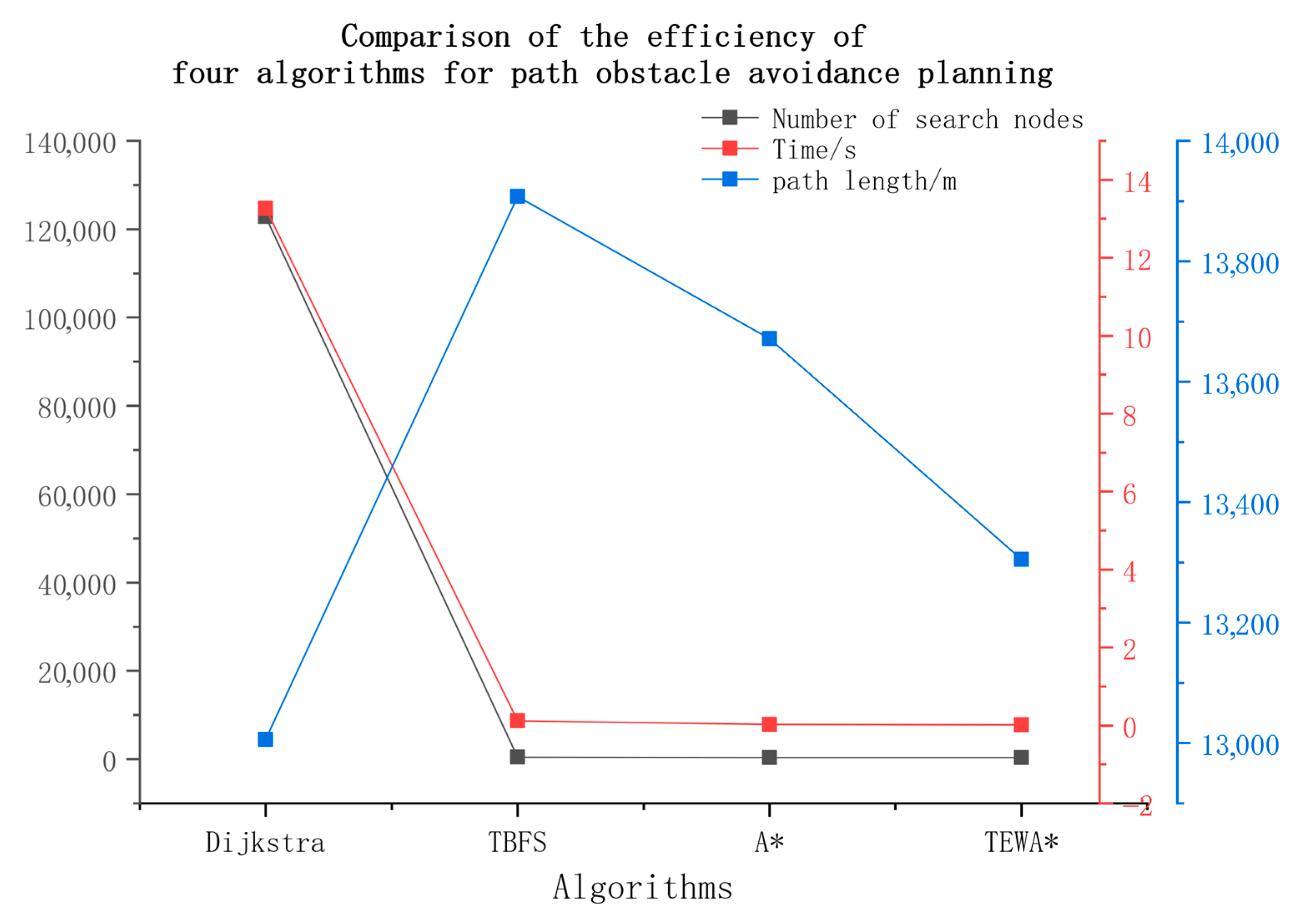
The comparison indexes and evaluation methods of the four algorithms can be evaluated and analyzed from the path length, running time, number of search nodes, path smoothness, applicability, and implementation complexity. Taking the running results of the four algorithms in Figure 13 as an example, under the condition of using the OpenList data structure of the hash table priority queue and the expansion of the eight-neighborhood model, the path obstacle avoidance planning efficiency of the four algorithms on the grid map is shown in

Table 5. Comparison of the efficiency of four algorithms for path obstacle avoidance planning.

Algorithms	Number of Search Nodes	Time/s	Path Length/m
Dijkstra	122,872	13.27	13,006.12
TBFS	457	0.12	13,907.40
A*	377	0.03	13,671.34
TEWA*	346	0.02	13,305.07

and Figure 14.

Based on the data in the comparison table of path obstacle avoidance planning efficiency for the four algorithms, the following analysis can be drawn:

(1) Under the conditions of using the same OpenList data structure and eight-neighborhood model, if the start and end points are the same and the same algorithm is used, the number of searched nodes is directly proportional to the search time. The more nodes searched, the lower the algorithm efficiency.

(2) The TEWA* algorithm outperforms the A* and TBFS algorithms in search efficiency and is significantly better than the Dijkstra algorithm. The Dijkstra algorithm yields the shortest path, but it consumes the longest time, far exceeding the time taken by other algorithms. The TEWA* algorithm excels in terms of the number of searched nodes, time, and path length.

The Dijkstra algorithm, when ignoring heuristics, can find the shortest global path from the start to the end point, but its search efficiency is low in large-scale raster maps. The TBFS algorithm searches very quickly but does not guarantee global optimality: if obstacles only become apparent later, it may lead to large detours or fall into local minima. The A* algorithm is suitable for path obstacle avoidance planning in flatter terrain scenarios. Compared to the TEWA* algorithm, its estimation accuracy for the current node and target node in pipeline path planning is insufficient. The TEWA* algorithm integrates the A* algorithm with terrain slope: in TEWA, $g\left(n\right)$ represents the actual cost from the start node to the current node, and $h\left(n\right)$ represents the heuristic estimate to the target node. By balancing both, it addresses the shortcomings of the Dijkstra algorithm and the GBFS algorithm. Therefore, considering both overall optimality and high efficiency, the TEWA algorithm is the optimal choice among the four algorithms for 3D raster terrain path obstacle avoidance planning.

6. Conclusions

This study focuses on the core issue of layout optimization for the underwater production system of deepwater oil and gas fields, and constructs a comprehensive model for the grouping of manifold positions and the planning of three-dimensional terrain pipeline routes. By integrating the K-means-ILP clustering algorithm and the TEWA path planning algorithm, a multimodal optimization framework was developed, achieving the collaborative optimization of well group division, manifold topology, and path layout. Experimental verification shows that in terms of the WCSS clustering validity index, the K-means-ILP algorithm improves by 23.6% compared to the traditional K-means algorithm; for complex terrain obstacles, the TEWA algorithm shortens the path length by 18.4% and reduces the calculation time by 37.2% compared to the Dijkstra, TBFS, and A* algorithms. Through the coupling manifold connection relationship optimization with dynamic programming, an efficient solution for the overall system layout under complex seabed terrain is ultimately formed, providing innovative technical support for deepwater oil and gas development. Key contributions and innovations are as follows:

(1) Model Construction: Developed a target grouping model minimizing drilling costs. Established a 3D obstacle-avoidance path planning model minimizing path length. Enhanced geological precision and engineering applicability through reservoir target inputs.

(2) Algorithm Design: Compared clustering algorithms (K-means, bipartite K-means, GA, K-means-ILP), validating K-means-ILP’s superiority in grouping stability and computational accuracy. Introduced TEWA* for 3D terrain path planning, significantly improving search efficiency and obstacle-avoidance capability.

In the future, time series DEM and geological disturbance analysis methods (such as the Monte Carlo disturbance model) will be introduced to assess the impact of geological uncertainties and long-term changes in the seabed on layout stability, thus extending the time series applicability of the current model.

Project funding number: 1500 m underwater Christmas tree and control system development.