Navigating the Trade-Offs: A Quantitative Analysis of Reinforcement Learning Reward Functions for Autonomous Maritime Collision Avoidance

Abstract

Autonomous navigation is critical for unlocking the full potential of Unmanned Surface Vehicles (USVs) in complex maritime environments. Deep Reinforcement Learning (DRL) has emerged as a powerful paradigm for developing self-learning control policies, yet the design of reward functions to balance conflicting objectives, particularly fast arrival at the target position and collision avoidance, remains a major challenge. The precise, quantitative impact of reward parameterization on a USV’s maneuvering behavior and the inherent performance trade-offs have not been thoroughly investigated. Here, we demonstrate that by systematically varying reward function weights within a framework relying on the Proximal Policy Optimization (PPO), it is possible to quantitatively map the trade-off between collision avoidance safety and mission time. Our results, derived from simulations, show that agents trained with balanced reward weights achieve target-reaching success rates exceeding 98% in dynamic multi-obstacle scenarios. Conversely, configurations that disproportionately penalize obstacle proximity lead to overly cautious behavior and mission failure, with success rates dropping to 22% due to workspace boundary violations. This work provides a data-driven methodological framework for reward function design and parameter selection in safety-critical robotic applications, moving beyond ad-hoc tuning towards a more structured parameter influence analysis.

1. Introduction

The increasing prevalence of Unmanned Surface Vehicles (USVs) in commercial, scientific, and security applications necessitates the development of robust autonomous navigation systems [1,2]. Deep Reinforcement Learning (DRL) has shown considerable promise for training control policies that can maneuver USVs in complex, dynamic maritime environments [3,4,5]. However, a fundamental challenge in applied DRL is reward engineering with respect to reward function shaping—the process of designing a reward function that correctly specifies the desired behavior [6,7]. This process is often treated as an unintuitive process, leading to extensive manual tuning and unpredictable outcomes [7,8]. For multi-objective tasks like autonomous navigation, which must simultaneously prioritize goal-reaching efficiency, safety, and operational constraints, the lack of a structured reward design methodology constitutes a significant bottleneck [9,10]. The quantitative impact of specific reward parameters on the emergent behavior of the agent and the inherent trade-offs between conflicting objectives remain insufficiently understood [3]. This paper addresses the gap by presenting a systematic, data-driven methodology for analyzing and engineering reward functions for USV collision avoidance. We use the Proximal Policy Optimization (PPO) algorithm [11] to train a series of agents within a maritime simulation environment built on Robot Operating System (ROS), Gazebo, and Virtual RobotX (VRX) [12]. By systematically varying the weights of reward components related to target-seeking and obstacle avoidance, we empirically map the performance landscape of the autonomous agent. This approach allows us to precisely quantify the trade-off between mission efficiency and safety margins. Our work moves beyond reporting singular, exemplary results and instead provides a reproducible framework for understanding how reward parameterization shapes agent behavior, offering a more robust and structured approach to designing safe and effective autonomous systems.

1.1. Background

In order to enable the USV with autonomous capabilities, a Guidance Navigation and Control (GNC) system consisting of guidance, navigation and control modules is typically employed across all USVs [13]. The system comprises a set of interconnected hardware and software elements that facilitate the execution of navigation and control tasks by the USV. Concurrently with a ground station, which may be located onshore, on a manned vessel, or reconnaissance aircraft, navigation data are collected and exchanged between the GNC system and the environment. Subsequently, the data are processed by the system, which results in a modification of the vessel’s state, thereby achieving the desired goal [4].

GNC systems represent a well-established area of research in the field of mobile robotics [4]. Navigation, the aim of which is to estimate the robot’s position and motion states with a high degree of precision, can be achieved through algorithms such as Simultaneous Localization and Mapping (SLAM) with an Extended Kalman Filter (EKF) or other Kalman filter variations based on sensor data [14,15]. These methods generate maps in real time, concurrently with the motion, and subsequently update them to categorize map sections according to their occupancy level and thus the hazard they pose to the USV [16,17,18]. Conventional map representations include occupancy grid maps, which encode the occupancy of each map in binary form. As an alternative, extended cost maps are utilized, facilitating the incorporation of supplementary information for each grid cell [15]. This approach enables the delineation of safety boundaries surrounding existing objects, for instance [19].

The approaches to the navigation task are usually based on these map representations and generate a path from the current position to the destination. In determining such a path, the objective is to identify a collision-free route that is as brief as possible, whilst considering secondary conditions such as waterway limitations or intermediate destinations [20].

The implementation of global path planning frequently involves the utilization of heuristic graph-based methods, which are capable of calculating a collision-free path on a grid map [4,21]. Examples of such algorithms include the Dijkstra algorithm-based A* and Theta* algorithms [21,22]. A disadvantage of these heuristic methods is the inherent increased computational effort for large maps, as well as the inability to include constraints such as energy optimality [21,22]. Furthermore, probabilistic path planning methods, such as Rapidly-Exploring Random Tree (RRT/RRT*), have been shown to offer advantages with regard to the optimality of the shortest path [23]. Only static objects can be included in path planning unless the path is to be updated regularly [21,22,24].

The avoidance of dynamic obstacles can be achieved through the implementation of strategies such as the Dynamic Window Approach (DWA) [4,25]. DWA involves the modification of path plans in response to detected obstacles while taking the inherent limitations of the ship’s dynamics into account during the replanning process [25]. The system selects an evasion trajectory once the Wave Adaptive Modular Vehicle (WAMV) comes within a predefined safety distance of an obstacle [25]. Notwithstanding the fact that this method has the capacity to prevent collisions by utilizing adequate safety factors, there are significant drawbacks. The DWA has been shown to be a temporary solution, as it does not predict the movements of other ships when selecting an evasion trajectory [4]. This may lead to safety-critical situations being maneuvered into. It is possible to mitigate this risk by adding so-called footprints of dynamic obstacles in cost maps, for example [25]. The presence of these footprints introduces additional costs in the predicted direction of the dynamic obstacle movement on the cost maps [4,24].

However, if constraints such as low energy consumption over the path, a limited jerk or a critical minimum distance to dynamic obstacles are also required to be fulfilled, trajectory planning becomes unavoidable [4]. Classic graph-based algorithms are often used for global path planning and local trajectory planning is carried out using artificial intelligence (AI) [26] or optimization-based algorithms in order to satisfy additional target quantities or respond to dynamically changing situations [27]. In general, many artificial intelligence approaches for path and/or trajectory planning have already been formulated and tested [27]. These have proven to be reliable approaches in complex environments with multiple constraints or cost-based maps. These approaches include, for example, Genetic Algorithms (GAs) [28] or Particle Swarm Optimizations (PSOs) [29,30], which will not be discussed further below, although more information is provided in the following review publications [27,31,32,33,34,35].

Model Predictive Controllers (MPCs) are commonly used optimization-based navigation methods that enable integrated guidance of USVs with simultaneous control [36,37]. By taking future states into account, reliable control performance of the dynamic system can be achieved, especially if disturbances are estimated [36,37]. In addition, the cost function can be individually designed, whereby the deviation from a global path, the proximity to an obstacle and the actuator power are typical cost function terms. In multi-obstacle scenarios, the predictions of several obstacle movements and additional costs for COLlision REGulation (COLREG) compliant behavior can also be integrated into MPCs [36]. The disadvantages of MPCs are their need for sufficiently accurate prediction models and their high computational efforts [38]. Furthermore, time and effort must also be invested in parameterizing the model and calibrating the cost function weights. This raises the motivation to develop a self-learning controller that takes over the task of guidance, including collision avoidance either completely or partially [36,37,39,40,41]. Corresponding approaches are presented in the following Section 1.2.

In addition to the combined guidance and control solutions already presented, such as the MPC, dedicated controllers also exist. Line-of-sight (LOS) systems using PID controllers can accurately follow planned trajectories [42,43]. Linear Quadratic Regulators (LQRs) offer optimality for linear systems [44]. Adaptive and learning-based methods, such as reinforcement learning or imitation learning, enable flexibility in dynamic environments, though often at the cost of poor interpretability or high training effort [45]. In over-actuated systems, thrust allocation can be used to convert USV motion requests into actuator commands, enabling the integration of additional optimization criteria such as actuator energy efficiency. Control allocation will be described in more detail in Section 2.1 [46].

1.2. Related Works

Beyond the aforementioned methods, Reinforcement Learning (RL)-based approaches are also employed in order to plan paths or trajectories (guidance), follow predefined references (control), or realize a combination of these tasks. Generally, various RL approaches are explored in the literature, and various scenarios are established. RL, particularly Deep Reinforcement Learning (DRL), offers an opportunity for controller development by enabling an agent to learn an optimal control policy autonomously through environmental interaction, thus bypassing the need for an explicit model in comparison to MPCs [14,47]. The RL approach might learn itself how to handle complex environments, demonstrating robust adaptability and the capacity to generalize from environment data [45]. Furthermore, RL is inherently suited for the sequential decision-making required for collision avoidance; its reward function can be engineered to optimize competing goals such as safety, efficiency, and rule adherence [47]. This paper applies an RL approach to automated ships; hence, key sources and their distinguishing features in the literature are presented.

An important distinguishing feature of different explorations in the literature is the variety of scenarios. Often, only a few scenarios are used for training and testing, whereby no scenario variations are performed, which may question the generalizability of the results. This section presents a selection of publications with regard to their application, RL approaches, and considered scenarios. When presenting the literature publications, it will also be specified if they explicitly consider COLREG [3].

For global path planning, Li et al. [48] propose a Deep Q-Network-based (DQN) approach augmented with Artificial Potential Fields (APFs) to guide USVs through static environments. Their method demonstrates adaptability to varying obstacle configurations and achieves efficient convergence in training. The integration of APF enhances the agent’s ability to avoid local minima, resulting in smoother trajectories and reduced path length compared to baseline DQN implementations. Zhao et al. [49] employ a Deep Deterministic Policy Gradient-based (DDPG) framework for navigation in randomized static environments. Their results indicate that the continuous action space of DDPG enables finer control over heading adjustments, leading to more stable path execution and lower cumulative reward variance across episodes. Both approaches are validated in simulations, showing reliable performance in static scenarios with moderate complexity.

In the domain of local path planning, Yang et al. [50] propose a Prioritized Experience Replay-enhanced Double Deep Q-Network (PER-DDQN) for dynamic obstacle avoidance. Their approach is evaluated in randomized scenarios with three dynamic obstacles and demonstrates stable convergence and improved sample efficiency. The agent successfully learns to avoid collisions while maintaining trajectory smoothness, outperforming standard DDQN baselines in terms of cumulative reward and training stability. For path following, Zhong et al. [51] employ a DDPG-based controller, which is validated both in simulation and on a full-scale USV. The method achieves low cross-track error and reduced rudder activity, indicating reliable trajectory tracking at minimal control effort. Deraj et al. [52] utilize a DQN-based strategy for reference tracking. While the discrete action space introduces occasional chattering due to limited control granularity, the method achieves comparable path-following accuracy to PID controllers and demonstrates robustness in structured environments.

Cui et al. [53] propose an enhanced collision avoidance strategy based on the DDPG algorithm, incorporating prioritized experience replay and Gated Recurrent Units (GRUs) to improve temporal representation and sample efficiency. Their method is evaluated in scenarios involving both static and dynamic obstacles, demonstrating trajectory smoothness and reduced collision rates. The agent achieves stable convergence and maintains low cross-track errors across multiple randomized test cases, outperforming baseline DDPG implementations in terms of reward accumulation and control stability. Xia et al. [45] employ the Proximal Policy Optimization (PPO) algorithm for dynamic collision avoidance in two fixed scenarios. The PPO-based agent exhibits robust performance with consistent avoidance behavior and minimal oscillations in heading control. Quantitative results show that the method achieves high success rates in obstacle avoidance and maintains efficient path execution, validating its applicability in constrained maritime environments.

Sun et al. [54] introduce a DRL-based collision avoidance framework that combines dueling networks, double Q-learning, prioritized experience replay, and noisy networks. Their approach models both static and dynamic obstacles and integrates COLREG into the reward function. Training is conducted in a highly randomized environment comprising over 20,000 configurations. The method achieved stable convergence and high average rewards, with improved generalization across scenarios.

Fan et al. [55] propose the NPD3QNU algorithm, a DRL-based collision avoidance method that integrates COLREG, ship domain modeling, and dynamic area constraints. The method combines dueling double DQN with noisy networks. In testing across multiple encounter scenarios, NPD3QNU achieved lower course deviation and rudder usage compared to baseline DQN, while maintaining COLREG compliance.

Chen et al. [3] present RLCA, a reinforcement learning-based collision avoidance algorithm that incorporates COLREG and maneuverability constraints. Their method uses a category-based exploration strategy and custom transition storage to improve learning stability and reward shaping. Compared to DQN and D3QN baselines, RLCA achieved higher average rewards and more stable convergence. In head-on encounters, the agent successfully avoided collisions with a minimum distance of 69.44 m and returned to its original course after avoidance.

Wang et al. [56] and Wang et al. [57] examine cooperative path planning and target search strategies for formations of USVs using deep reinforcement learning. Their methodologies employ centralized and distributed learning frameworks to coordinate multiple agents in dynamic environments. Empirical evaluations indicate that the proposed systems enable consistent inter-agent spacing and effective obstacle avoidance, while maintaining trajectory coherence. The learning-based controllers demonstrate convergence within a reasonable number of training episodes and exhibit stable behavior under varying initial conditions. Quantitative metrics, such as average path length and formation deviation, suggest that the approaches are competitive with conventional rule-based coordination schemes, particularly in scenarios involving moderate environmental complexity.

1.3. Contribution

Based on the literature review, the most common encounter situations were selected and the focus was placed on scenario variability. Three scenarios presented in this work apply PPO to address collision avoidance tasks in maritime environments. They are trained using randomized scenario variations to promote generalization across diverse operational conditions. The agent’s performance is assessed based on success rates in reaching the target destination collision-free, average velocities and minimum distances to both static and dynamic obstacles. To systematically investigate the influence of algorithmic and environmental parameters, multiple scenario configurations and reward function variations are analyzed using statistical investigations such as box plots and scatter plots. This enables a quantitative assessment of policy sensitivity and robustness. It is noted that several existing studies in the literature primarily report exemplary results from selected scenarios, without providing a broader statistical analysis of parameter effects or variability across trials. The present work aims to address this gap by incorporating structured evaluation and comparative metrics across randomized conditions. While the experimental scenarios, particularly CA2, are designed to rebuild common encounter situations such as head-on or crossing maneuvers, this work does not yet explicitly enforce or integrate COLREG. The agent’s maneuvering policies are purely emergent, learned exclusively from the reward terms defined in Section 2.2.3, which do not presently contain any specific component to penalize non-compliant actions. This represents a deliberate limitation to isolate the effects of the core reward parameters. Future investigations, as discussed in the conclusion, shall focus on integrating these crucial maritime rules.

2. Methodology

This section presents the methodological framework used to investigate RL-based control strategies for USVs. Section 2.1 introduces the architecture of the training framework, including the simulation environment, agent–environment interaction, and thrust allocation mechanisms. Section 2.2 defines the reinforcement learning problem formulations for both path following and collision avoidance tasks, detailing the respective observation and action spaces, reward functions and scenario generation procedures.

2.1. Framework Architecture

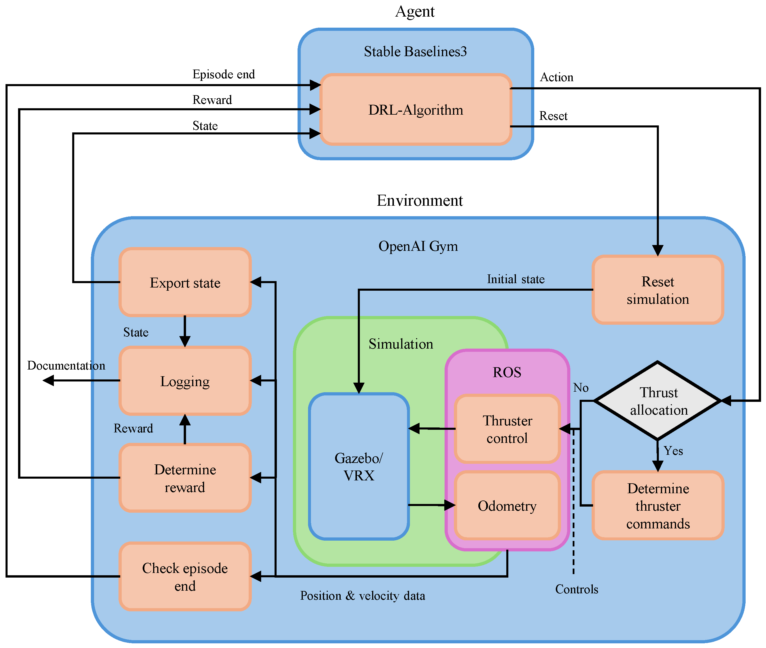
The architecture of the RL training framework is illustrated in Figure 1. It shows the interaction between the agent and the simulation environment during training, as well as a simplified representation of the signal flows. The agent is implemented using DRL algorithms from Stable Baselines3 [58], while the environment is based on OpenAI Gym [59]. At the core of the environment is the simulation realised in Virtual RobotX (VRX) [12], which approximates the behavior of USV operating in complex ocean environments. VRX enables the integration of ship models, such as the WAMV and other static or dynamic objects, into the simulation environment and enables the creation of scenarios. Communication between the RL environment and the simulation is handled via Robot Operating System (ROS) [60]. Through this interface, control commands are sent to the WAMV actuators, and odometry data are retrieved. These data are used to compute the current state, reward, and episode termination condition. All relevant data are logged for analysis and visualization.

The agent interacts with the environment using the standard reset and step methods of OpenAI Gym. At the beginning of each episode, the environment and simulation are reset to their initial states. If thrust allocation is enabled, the selected action is first translated into actuator-level control commands, ensuring that the WAMV’s propulsion system is driven in accordance with its physical constraints and maneuvering capabilities. The resulting state and reward are then returned to the agent. If thrust allocation is disabled, the agent would control the thrusters directly.

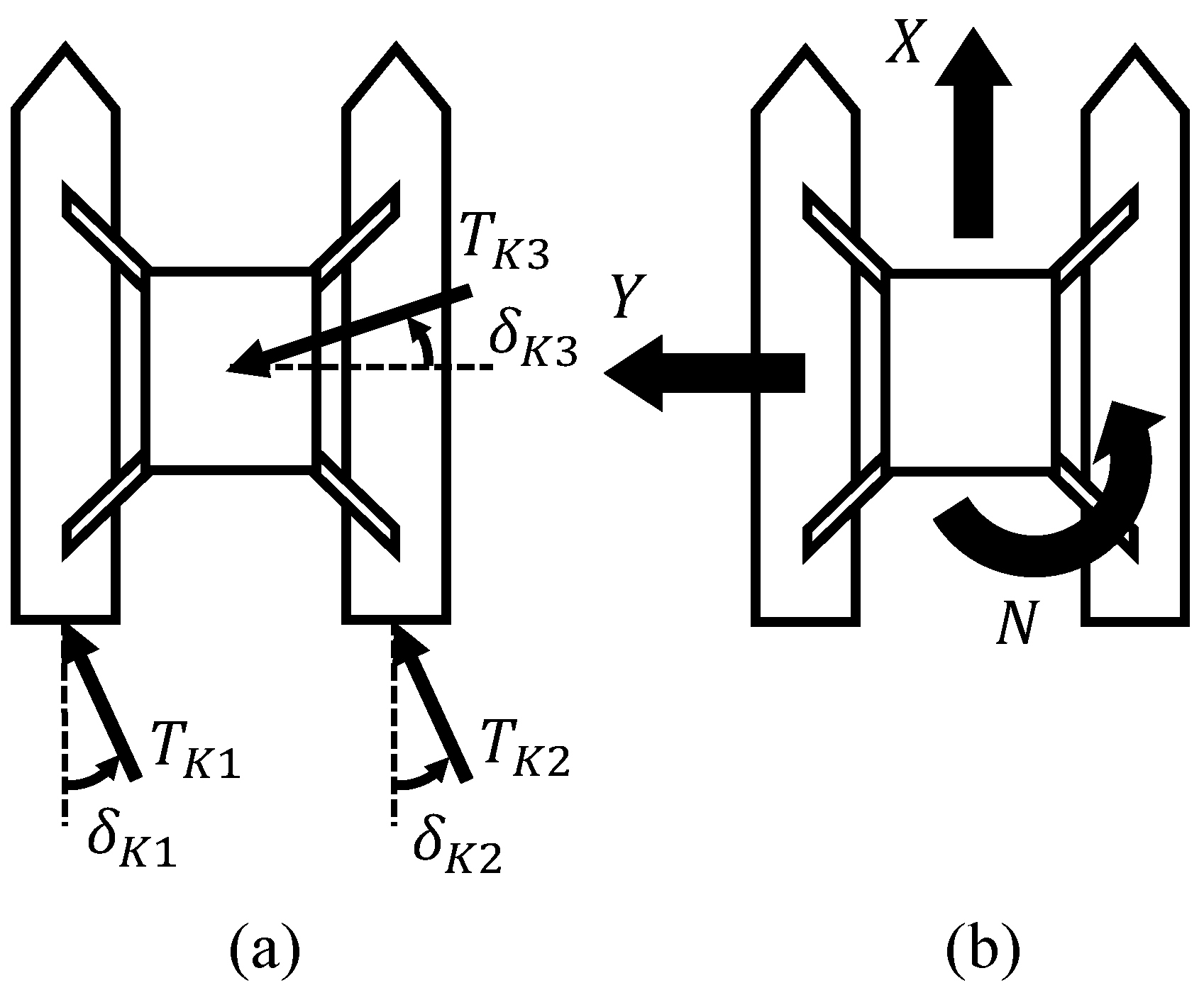
Control allocation is used to exploit actuator redundancy in over-actuated marine vessels, enabling the system to distribute control efforts optimally among multiple thrusters. This enhances flexibility, fault tolerance and performance by solving an optimization problem that maps desired virtual forces to individual actuator commands, including thrust magnitudes and azimuth angles. Using the over-actuated WAMV in T1 configuration (see Figure 2), the optimization problem for the thrust allocation can be set up as follows (see Equation (1)) [12,46].

$$\begin{array}{cc}\hfill \mathrm{minimize}& J(\mathit{\delta },\mathit{u},\mathit{s})=\sum W_i\left(u_i\right)+{\mathit{s}}^T\mathit{Q}\mathit{s}+\hfill \\ \hfill & {(\mathit{\delta }-{\mathit{\delta }}_0)}^T\Omega (\mathit{\delta }-{\mathit{\delta }}_0)\hfill \\ \hfill \mathrm{subject}\mathrm{to}& \mathit{s}=\mathit{\tau }-\mathit{B}\left(\mathit{\delta }\right)\mathit{u}\hfill \\ \hfill & {\mathit{u}}_{min}\le \mathit{u}\le {\mathit{u}}_{max}\hfill \\ \hfill & {\mathit{\delta }}_{min}\le \mathit{\delta }\le {\mathit{\delta }}_{max}\hfill \\ \hfill & \Delta {\mathit{\delta }}_{min}\le \mathit{\delta }-{\mathit{\delta }}_0\le \Delta {\mathit{\delta }}_{max}\hfill \end{array}$$

(1)

The first term $\sum W_i\left(u_i\right)$ within the cost function describes the costs of the power consumption of the individual actuator thrust forces $u_i$. Second, the term ${\mathit{s}}^T\mathit{Q}\mathit{s}$ penalizes the error $\mathit{s}$ between the virtual and actual generalized forces. The diagonal matrix $\mathit{Q}>0$ includes costs for the error s and they are assigned sufficiently high, so that $s\approx 0$ whenever possible. The third term in the cost function represents the cost for the rate of change of the azimuths, because large changes in azimuth angle are not desirable nor even physically achievable and are therefore penalized with costs. The costs for the change rate of each individual thruster are described in the matrix $\Omega$. The cost function is subject to equality and inequality constraints. The equality constraint $\mathit{s}=\mathit{\tau }-\mathit{B}\left(\mathit{\delta }\right)\mathit{u}$ is used to introduce the slack variable. The second constraint ${\mathit{u}}_{min}\le \mathit{u}\le {\mathit{u}}_{max}$ limits the minimum and maximum forces that can be produced by the actuators. Next, ${\mathit{\delta }}_{min}\le \mathit{\delta }\le {\mathit{\delta }}_{max}$ constraints the positive and negative azimuth angles of the individual thrusters. The final inequality constraint $\Delta {\mathit{\delta }}_{min}\le \mathit{\delta }-{\mathit{\delta }}_0\le \Delta {\mathit{\delta }}_{max}$ represents the hard limit of the technically achievable turning speed of the azimuth thrusters. Solving this cost function is done via the minimize function of the SciPy library [61]. The library offers multiple solvers for a wide range of optimization problems. The Sequential Least SQuares Programming (SLSQP) solver was selected due to its capability to handle both bound constraints and general equality or inequality constraints, which is essential for the formulation of the control allocation problem. Moreover, according to the official documentation, SLSQP is recognized for its robustness and flexibility in solving non-convex optimization problems, making it a suitable choice for the nonlinearities present in the system. The parameters used for the thrust allocation can be found in Appendix A within

Table A1. Cost function parameters for the thrust allocation algorithm.

Parameter	Qii	Ωii	umax	umin	umax/min	Δδmax/min
Value	1	0.001	250 N	−100 N	$\pm \pi /4$ rad	$\pm 0.05$ rad

[46,61].

2.2. Scenario Overview and Definition of the Reinforcement Learning Problems

This study investigates the application of RL methods to the maritime maneuvering task of collision avoidance (CA). To systematically evaluate the performance and generalizability of the trained agents, three distinct experimental scenarios were designed. The following provides an overview of these scenarios, which progressively increase in complexity. The specific RL problem formulation for each case, including the definition of observation spaces and reward functions, will be detailed in subsequent sections.

• Collision Avoidance (CA)

  –

  CA1—Static Obstacle Avoidance:

  The USV is tasked with navigating towards a target destination while safely maneuvering around one or more stationary obstacles.

  –

  CA2—Dynamic Obstacle Avoidance:

  This scenario involves the safe avoidance of a single, moving obstacle, requiring the USV to anticipate the obstacle’s future path.

  –

  CA3—Multi-Hindrance Environment:

  A complex scenario requiring the USV to navigate safely through an environment containing a combination of both static and dynamic obstacles.

The agents in all three scenarios are trained using the PPO algorithm. As a policy-gradient method, PPO is well-suited for problems with continuous action spaces, such as the virtual forces for the thrust allocation [11]. Furthermore, it is known for its robust convergence and training stability, which it achieves through a clipped objective function that prevents destructively large policy updates [11]. For training, the default hyperparameters from the Stable Baselines3 library are used, which are listed in Appendix A within

Table A2. Hyperparameters for the PPO algorithm.

Parameter	Value
Learning rate	3 $\times {10}^{-4}$
Timesteps per update	2048
Batch size	64
Number of epochs	10
Discount factor	0.99
GAE bias vs. variance factor	0.95
Clip range	0.2
Clip range for value function	None
Entropy coefficient	0
Value function coefficient	0.5
Max. value for gradient clipping	0.5

[58]. To ensure a reproducible baseline, allowing the analysis to focus on the design and trade-offs of the reward function itself, no hyperparameter variations are performed across the presented results. However, it is acknowledged that the agents’ performances are inherently linked to this hyperparameter configuration. A dedicated optimization of hyperparameters, such as the learning rate, batch size, or number of epochs, could potentially influence the results, for instance, by improving the optimality of the final learned policy [62,63,64].

2.2.1. Action Space

The RL agent’s action vector ${\mathbf{a}}_{CA}$ in the CA scenarios is defined via thrust allocation to ensure generalizability across motor configurations:

$${\mathbf{a}}_{CA}={[X_{CA},Y_{CA},N_{CA}]}^T$$

(2)

where $X_{CA}$ and $Y_{CA}$ are the surge and sway forces, and $N_{CA}$ is the yaw moment in the body-fixed frame (see Figure 2).

2.2.2. Observation Space

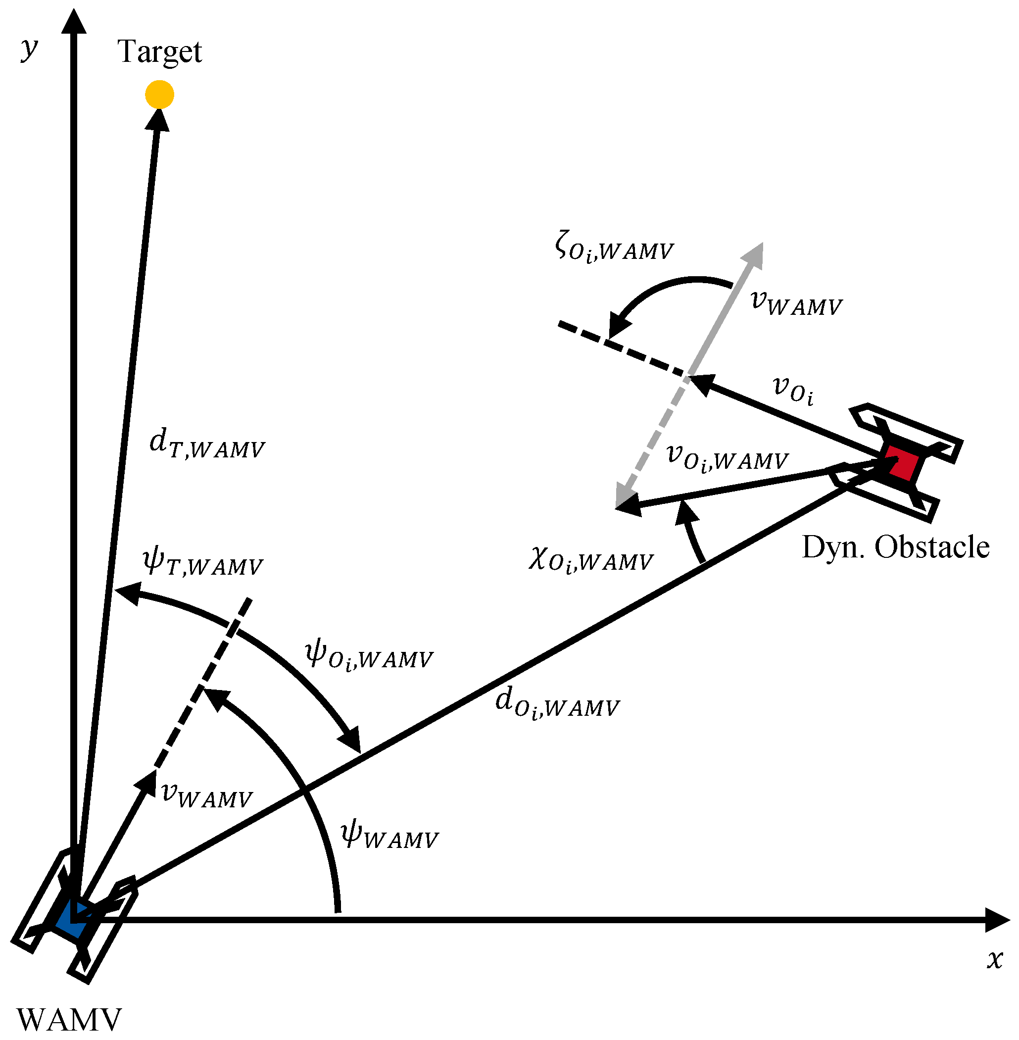
The observation vector ${\mathbf{o}}_{CA}$ in the CA scenarios comprises the target’s state and the states of one or more obstacles, all expressed relative to the WAMV. It is defined in Equation (3), and its components are visualized in Figure 3.

$$\begin{array}{cc}\hfill {\mathbf{o}}_{CA}=& \left[d_{T,WAMV},{\psi }_{T,WAMV},d_{O_i,WAMV},{\psi }_{O_i,WAMV},v_{O_i,WAMV},\right.\hfill \\ \hfill & {\left.{\chi }_{O_i,WAMV},{\zeta }_{O_i,WAMV}\right]}^T\hfill \end{array}$$

(3)

Addressing transfer to a physical system, which requires robust state estimation and sensor fusion, remains a critical step for future work. $d_{T,WAMV}$ denotes the Euclidean distance between the target point and the WAMV, while ${\psi }_{T,WAMV}$ represents the relative angle from the WAMV to the target point. Similarly, $d_{O_i,WAMV}$ and ${\psi }_{O_i,WAMV}$ are the corresponding values for an obstacle $O_i$. Furthermore, $v_{O_i,WAMV}$ is the magnitude of the obstacle’s linear velocity relative to the WAMV, ${\chi }_{O_i,WAMV}$ is the angle between this relative velocity vector and the distance vector ${\mathbf{d}}_{O_i,WAMV}$, and ${\zeta }_{O_i,WAMV}$ describes the relative course angle between the WAMV and the obstacle.

The Euclidean distance $d_{T,WAMV}$ between the WAMV’s position $[x_{WAMV},y_{WAMV}]$ and the target position $[x_T,y_T]$ is calculated as follows:

$$d_{T,WAMV}=\sqrt{{(x_T-x_{WAMV})}^2+{(y_T-y_{WAMV})}^2}$$

(4)

The Euclidean distance to an obstacle, $d_{O_i,WAMV}$, is calculated analogously using the obstacle’s position $\left[x_{O_i},y_{O_i}\right]$.

The relative angle to the target point ${\psi }_{T,WAMV}$ is determined as follows:

$${\psi }_{T,WAMV}=\mathrm{atan}2(d_{T,WAMV,y},d_{T,WAMV,x})-{\psi }_{WAMV}$$

(5)

Here, $d_{T,WAMV,x}$ and $d_{T,WAMV,y}$ correspond to the x- and y-components of the distance vector ${\mathbf{d}}_{T,WAMV}$ and ${\psi }_{WAMV}$ is the yaw angle of the WAMV. Similarly, the relative angle to an obstacle ${\psi }_{O_i,WAMV}$ is determined, but with the distance vector from the WAMV to the obstacle ${\mathbf{d}}_{O_i,WAMV}$.

The magnitude of the relative velocity of an obstacle, $v_{O_i,WAMV}$, is calculated as follows:

$$v_{O_i,WAMV}=\sqrt{{(v_{O_i,x}-v_{WAMV,x})}^2+{(v_{O_i,y}-v_{WAMV,y})}^2}$$

(6)

where $v_{O_i,x}$, $v_{O_i,y}$, $v_{WAMV,x}$ and $v_{WAMV,y}$ denote the x- and y-components of the absolute velocity of the obstacle, respectively, the WAMV. These velocity components are derived from the vehicles’ odometry data.

The angle ${\chi }_{O_i,WAMV}$ represents the angle between the relative velocity vector of the obstacle ${\mathbf{v}}_{O_i,WAMV}$ and the distance vector from the obstacle to the WAMV, $-{\mathbf{d}}_{O_i,WAMV}$. It is computed as follows:

$$\begin{array}{cc}\hfill {\chi }_{O_i,WAMV}=& \mathrm{atan}2(v_{O_i,WAMV,y},v_{O_i,WAMV,x})\hfill \\ \hfill & -\mathrm{atan}2(-d_{O_i,WAMV,y},-d_{O_i,WAMV,x})\hfill \end{array}$$

(7)

In addition to ${\chi }_{O_i,WAMV}$, the relative course angle ${\zeta }_{O_i,WAMV}$ is used to distinguish between head-on and overtaking the encounter. It is defined as follows:

$${\zeta }_{O_i,WAMV}=\mathrm{atan}2(v_{O_i,y},v_{O_i,x})-\mathrm{atan}2(v_{WAMV,y},v_{WAMV,x})$$

(8)

Within the scope of the paper, the observation vector is always defined in such a way that all objects in the scenario can be observed simultaneously. If there are fewer objects within the scenario variation, the missing objects are defined in the observation space so that they have no influence on the agent anymore. For example, the distance is set to a high value so that the agent does not expect any danger of collision. For a generalized formulation, a maximum number of, for example, 5 objects could be defined in the observation function, whereby the nearest objects within a predefined radius are considered. ${\mathbf{o}}_{CA}$ is populated with ground-truth state information directly from the simulation environment. This idealization omits the significant challenges of real-world perception, such as sensor noise, data asynchronicity and latencies from processing GPS, IMU, and LiDAR/radar data. Consequently, the agent’s performance in this study relies on perfect state awareness, and a “sim-to-real” gap must be assumed.

2.2.3. Reward Function

The reward function $R_{CA}$ in the collision avoidance scenarios are defined similarly for CA1, CA2 and CA3. Its primary purpose is to reward the agent for navigating safely and efficiently towards the target point. The reward function used and analyzed in this work consists of three terms:

$$R_{CA}=R_{CA,TC}+R_{CA,OA}+R_{CA,T}$$

(9)

Here, $R_{CA,TC}$ is a reward term for the target course, $R_{CA,OA}$ is a penalty term for obstacle avoidance and $R_{CA,T}$ is a reward term for reaching the target destination. The terms $R_{CA,TC}$ and $R_{CA,OA}$ are calculated at each time step and passed to the agent, whereas $R_{CA,T}$ is only given at the end of a successful training episode. A COLREG Reward is not considered in this paper, but should be included in future investigations.

The target course reward term $R_{CA,TC}$ is intended to help the agent steer towards the goal position. The target is to reward the agent when the velocity vector of the WAMV points in the direction of the target. This target point will be defined in the scenario generation. Compared to a target course reward term that only includes a reduction in distance to the target, using the velocity vector incorporates the advantage that also traveling in the intended direction is being rewarded. Moreover, the agent’s actions influence the velocity more immediately than the distance due to the integral relationship between speed and position. The base for calculating the target course reward is the relative heading angle ${\chi }_{T,WAMV}$ between the WAMV’s velocity vector and the distance vector from the WAMV to the target $d_{T,WAMV}$. It is computed analogously to ${\chi }_{O_i,WAMV}$. Since a small relative heading angle is desirable, smaller angles are rewarded more strongly. To achieve this, an exponential function is combined with a cosine function. The target course reward term is defined as follows:

$$R_{CA,TC}={\gamma }_{CA,TC}·exp\left(\mathit{\delta }\left({\displaystyle \frac{cos\left({\chi }_{T,WAMV}\right)+1}{2}}-1\right)\right)$$

(10)

Here, ${\gamma }_{CA,TC}$ is a weighting factor that determines the influence of this term relative to the others in the total reward function. The cosine function ensures that the reward is maximal when the WAMV is heading directly toward the target and minimal when it is moving in the opposite direction. The exponential function causes the reward to decrease more sharply for larger deviations from the target course. The parameter $\delta$ controls how quickly the reward drops off; higher values of $\delta$ lead to significantly lower rewards even for small deviations.

The obstacle avoidance penalty term $R_{CA,OA}$ is designed to reward the agent when avoiding obstacles early and maintain a safe distance. The agent is penalized when it gets too close to obstacles. The distances $d_{O_i,WAMV}$ between the WAMV and all obstacles are used for this calculation. These distances are scaled using an exponential function and summed, resulting in the following penalty term:

$$R_{CA,OA}=-{\gamma }_{CA,OA}\sum _{i}exp\left(-{\left({\displaystyle \frac{d_{O_i,WAMV}}{\beta }}\right)}^4\right)$$

(11)

The exponential function with a negative exponent ensures that the agent is penalized more strongly as it gets closer to an obstacle. The parameter $\beta$ controls the effective range of the penalty. A smaller $\beta$ allows the WAMV to get closer to an obstacle before the penalty increases significantly. The influence of this penalty term on the total reward is scaled by the weighting factor ${\gamma }_{CA,OA}>0$.

The episode end reward term is intended to align the agent with its primary objective: to navigate the WAMV safely and without collisions to the target point. This term rewards the agent when the WAMV reaches the target point and penalizes it otherwise, either in the case of a collision with an obstacle or if the WAMV leaves the operational area.

The episode end reward term is defined as follows:

$$R_{\mathrm{CA},\mathrm{T}}=\left\{\begin{array}{cc}{\gamma }_{\mathrm{CA},\mathrm{T},\mathrm{E}}\hfill & \mathrm{if}\mathrm{the}\mathrm{target}\mathrm{is}\mathrm{reached}\hfill \\ -{\gamma }_{\mathrm{CA},\mathrm{T},\mathrm{F}}\hfill & \mathrm{if}\mathrm{collision}/\mathrm{leaving}\mathrm{operational}\mathrm{area}\hfill \\ 0\hfill & \mathrm{otherwise}\hfill \end{array}\right.$$

(12)

Here, ${\gamma }_{\mathrm{CA},\mathrm{T},\mathrm{E}}>0$ is a constant reward value for successfully reaching the target point, and ${\gamma }_{\mathrm{CA},\mathrm{T},\mathrm{F}}>0$ is a constant penalty value for failure due to a collision or leaving the operational area. These values are chosen to be significantly larger than the maxima of the other reward terms to ensure that the agent does not only learn to take short-term beneficial actions, but instead optimizes its policy toward this overarching goal.

2.2.4. Scenario Generation

In general, agents are trained without disturbances at the beginning of all three scenarios, and then the best-performing agents are trained with disturbances. When enabled, VRX wind and wave models are used [12]. The wind is set to a mean value of $6\mathrm{m}/\mathrm{s}$ and a variance of $6\mathrm{m}/\mathrm{s}$, which corresponds to strong winds with a force of up to 6 on the Beaufort force scale. The wave model was configured with a nominal period of $5\mathrm{s}$ and a gain value of 1.

CA1—Static Obstacle Avoidance

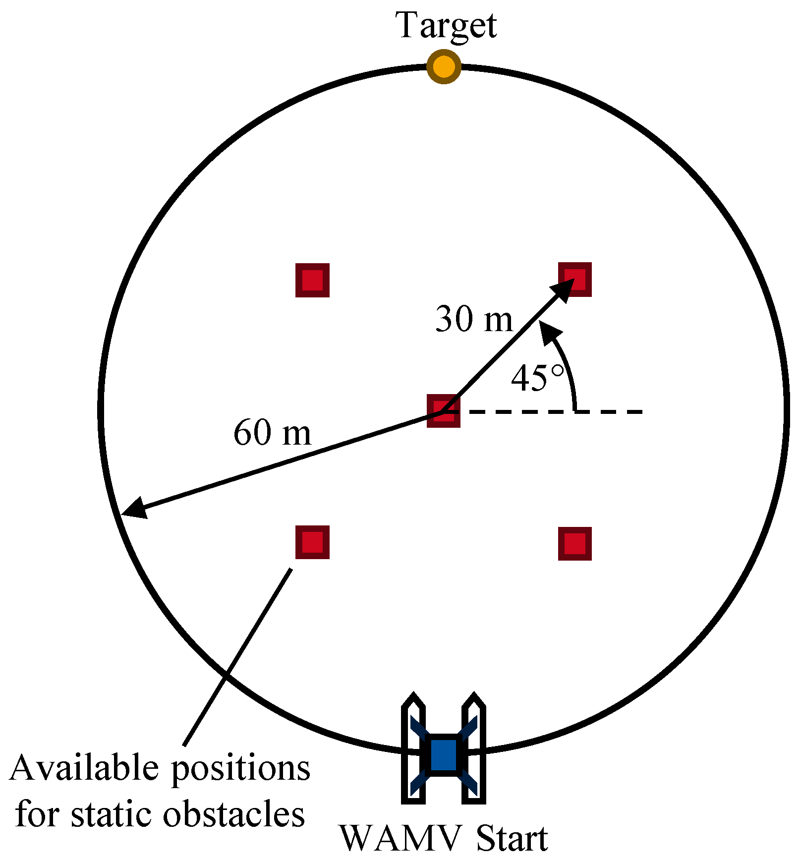
In the first scenario, between one and three static obstacles are randomly placed in five predefined positions. These obstacles represent stationary maritime elements such as buoys that may obstruct the vessel’s path. The WAMV initiates its maneuver from a circular starting area with a radius of 60 m and is tasked with reaching a designated target point located diametrically opposite. The five potential buoy positions include the center of the circle and the vertices of a square inscribed within a smaller circle of 30 m radius at the same center point. At the beginning of each episode, the number of buoys is randomly selected within the range of one to three and distributed randomly among the available positions (see Figure 4). The navigable area is extended by a 40 m tolerance zone, resulting in a total radius of 100 m. An episode ends when the goal is reached, a collision occurs, the area is exited or the step limit of 300 steps is reached.

During training, a total of at least 800 episodes are executed. To facilitate initial learning, the agent is trained without obstacles for the first 150 episodes. This approach allows the agent to focus exclusively on goal-reaching behavior in the early stages. This form of curriculum learning has demonstrated improved learning performance and convergence during development. The minimum number of episodes results from a total training budget of 240,000 steps, which corresponds to 800 episodes with a maximum of 300 steps each. In practice, however, episodes often terminate before reaching the step limit. Therefore, additional episodes are executed until the full step budget of 240,000 steps is exhausted. This training procedure and step-based episode extension apply analogously to all subsequent scenario descriptions.

CA2—Dynamic Obstacle Avoidance

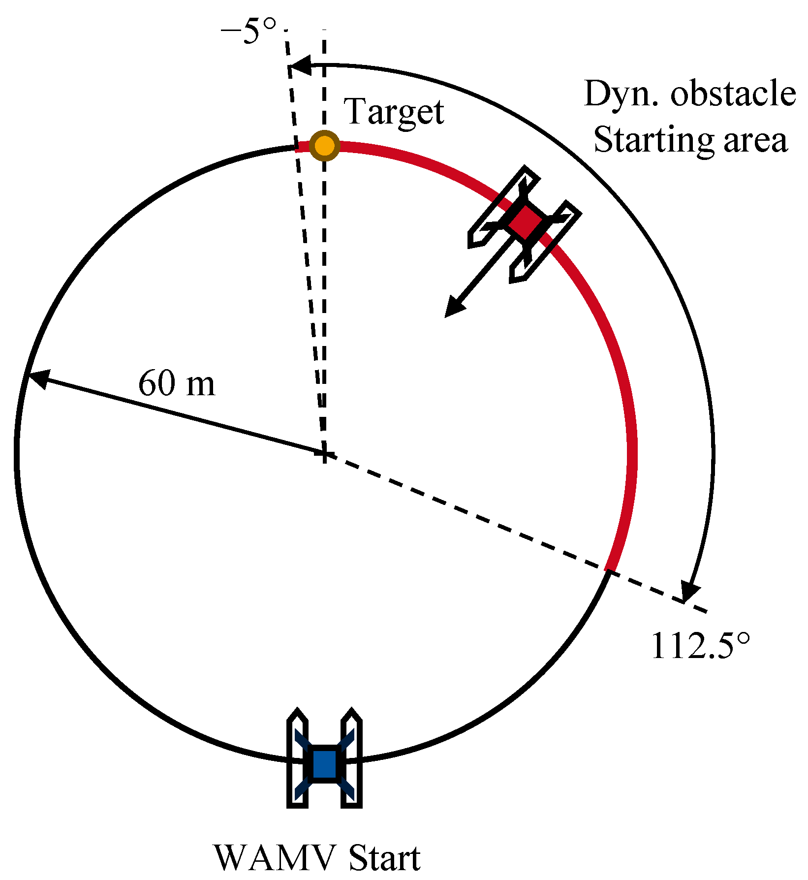
In this scenario, the agent is trained to avoid a single dynamic obstacle. The WAMV starts at a random position on a circular area with a radius of 60 m and aims to reach a goal located on the opposite side. A dynamic obstacle is randomly placed on the circumference of the 60 m circle within a predefined angular range between $-5^{\circ }$ and $+112.5^{\circ }$, and moves linearly toward the center at a constant speed, simulating either a head-on or crossing give way encounter with regard to COLREG. The obstacle’s velocity is randomly sampled from a uniform distribution between 0.25 m/s and 2.25 m/s. A schematic representation of this scenario is shown in Figure 5.

The navigable area is extended by a 40 m tolerance zone, resulting in a total radius of 100 m. An episode terminates when the goal is reached, a collision occurs, the area is exited, or the step limit of 300 steps is exceeded. During training, a total of at least 800 episodes are executed.

Key Performance Indicators (KPIs) are widely employed to characterize the dynamic interaction between two vehicles and to assess the risk level of traffic encounter situations based on predefined thresholds [65]. Among various KPIs, Time to Collision (TTC) and Post Encroachment Time (PET) are particularly relevant for complex dynamic scenarios and are well-suited for evaluating the performance of trained models in this work in dynamic scenarios. TTC represents the remaining time before a potential collision occurs under the assumption that both ships maintain their current speed and heading. For curved trajectories, TTC can be adapted as the Euclidean distance between the two ships divided by the projection of their relative velocity onto the line connecting their positions:

$$\mathrm{TTC}={\displaystyle \frac{d}{|v_{\mathrm{rel}}|}},$$

(13)

where $d= \parallel {\mathbf{p}}_1-{\mathbf{p}}_2{\parallel }_2$ denotes the distance between the two ships, and

$$v_{\mathrm{rel}}=({\mathbf{v}}_1-{\mathbf{v}}_2)·{\displaystyle \frac{{\mathbf{p}}_1-{\mathbf{p}}_2}{d}}$$

(14)

is the relative velocity component along the line of sight between them. Here, ${\mathbf{p}}_1$ and ${\mathbf{p}}_2$ are the position vectors, and ${\mathbf{v}}_1$ and ${\mathbf{v}}_2$ are the velocity vectors of the two ships, respectively.

PET is defined as the time gap between the moment when one ship leaves a shared conflict zone and the moment when the other ship enters the same zone, where their planned trajectories intersect:

$$\mathrm{PET}=t_{\mathrm{entry}}^{\left(2\right)}-t_{\mathrm{exit}}^{\left(1\right)},$$

(15)

where $t_{\mathrm{exit}}^{\left(1\right)}$ and $t_{\mathrm{entry}}^{\left(2\right)}$ represent the respective exit and entry times of the conflict area.

Lower TTC and PET values correspond to more critical encounter situations, indicating a higher collision risk. In each scenario, TTC is updated at every time step, whereas PET is defined only when the two trajectories intersect within a shared conflict zone. The analysis focuses on the minimum TTC attained within the scenario and the PET, as these quantities capture the most critical situation.

CA3—Multi-Hindrance Scenario

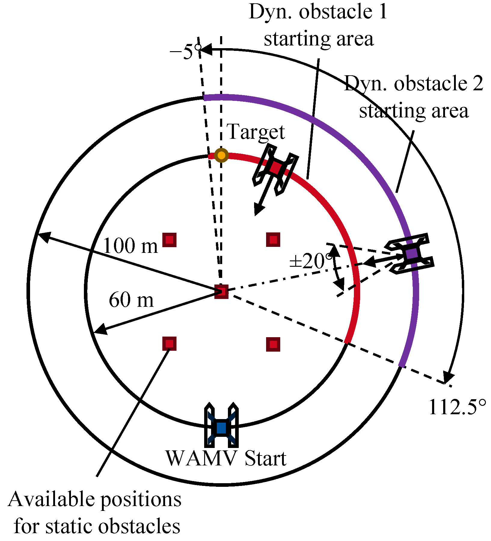
This scenario extends the previous setups by combining elements from Scenario CA1 and CA2. The agent must learn to avoid multiple dynamic obstacles as well as a static one. A schematic overview of the scenario is shown in Figure 6.

One static obstacle is randomly placed at one of five predefined positions, identical to those used in Scenario CA1. These positions include the center of the circle and the vertices of a square inscribed within a smaller circle of 30 m radius centered at the same point. The WAMV, the target position, and the first dynamic obstacle are initialized as in Scenario CA2, on a circle with a radius of 60 m. The first dynamic obstacle moves linearly toward the center of the circle at a constant, randomly selected positive speed. A second dynamic obstacle is placed on a larger circle (radius 100 m), within an angular sector from $-5^{\circ }$ to $112.5^{\circ }$ relative to the center-goal line. It also moves linearly with a random speed between 0.25 m/s and 2.25 m/s, but its course may deviate by up to $\pm {20}^{\circ }$ from the centerline, allowing for more diverse encounter situations.

To simplify the simulation, obstacle avoidance behavior is disabled for the obstacles. If any two obstacles come within 8 m of each other, the dynamic ones are stopped to prevent collisions that could disrupt the simulation. The navigable area is extended in comparison to the CA1 and CA2 scenarios, resulting in a total radius of 280 m to allow the agent greater room for maneuver in the more complex scenario. Episodes end under the same conditions as in CA2. The step limit is also doubled to 600 compared to CA1 and CA2. During training, a total of at least 800 episodes are executed. To facilitate initial learning, the agent is trained without obstacles for the first 150 episodes.

3. Results and Discussion

This section presents the training results of the various scenarios presented with their respective RL formulations. For validation, the agents are executed in the same scenario in which they were trained over 200 episodes. The step limit per episode is identical to the training. However, a different variation of the scenarios is used in the evaluation, so that, for example, obstacle speed or disturbance variables such as wind and waves may be modified compared to the training. To ensure comparability of the evaluation results across all scenarios and agents, the same set of 200 evaluation variations is used for all agents of one scenario. To analyze the impact of reward shaping on the agent’s behavior, multiple variations of the reward weights ${\gamma }_{\mathrm{CA},\mathrm{OA}}$ (obstacle avoidance) and ${\gamma }_{\mathrm{CA},\mathrm{TC}}$ (target course) are considered. While these parameters are varied, the remaining parameters are held constant throughout all experiments: $\delta =5$, $\beta =25$, ${\gamma }_{\mathrm{CA},\mathrm{T},\mathrm{E}}=20$ (goal-reaching reward), and ${\gamma }_{\mathrm{CA},\mathrm{T},\mathrm{F}}=20$ (failure penalty). For reasons of computational effort and in view of the trade-off focus of this article, a full factorial review of all parameters was not performed. In a multi-term reward function, the agent’s emergent policy is governed by the relative dependencies and ratios between the competing reward components, not their absolute magnitudes. Therefore, the most direct method to analyze the high-level trade-off between safety and efficiency is to fix the function shapes ($\delta$, $\beta$) and systematically vary the principal weights of the competing terms, ${\gamma }_{CA,TC}$ and ${\gamma }_{CA,OA}$.

The variation name encoding of these parameter combinations is summarized in

Table 1. Agent’s configuration encoding for variations of ${\gamma }_{\mathrm{CA},\mathrm{OA}}$ and ${\gamma }_{\mathrm{CA},\mathrm{TC}}$ and disturbance variations used in the reward function.

Configuration Encoding	Parametrization
C_1_Y	${\gamma }_{\mathrm{CA},\mathrm{OA}}=0.1$
C_2_Y	${\gamma }_{\mathrm{CA},\mathrm{OA}}=1$
C_3_Y	${\gamma }_{\mathrm{CA},\mathrm{OA}}=5$
C_X_1	${\gamma }_{\mathrm{CA},\mathrm{TC}}=0.025$
C_X_2	${\gamma }_{\mathrm{CA},\mathrm{TC}}=0.05$
C_X_3	${\gamma }_{\mathrm{CA},\mathrm{TC}}=0.1$

. This setup enables a focused investigation of the trade-offs between obstacle avoidance, target-reaching behaviors and disturbance resilience. Disturbance configurations such as wind and waves are examined to assess the robustness of the learned policy.

3.1. Scenario CA1—Static Obstacle Avoidance

In the CA1 scenario, the agent is evaluated in a static obstacle avoidance task, as detailed in Section 2.2.4.

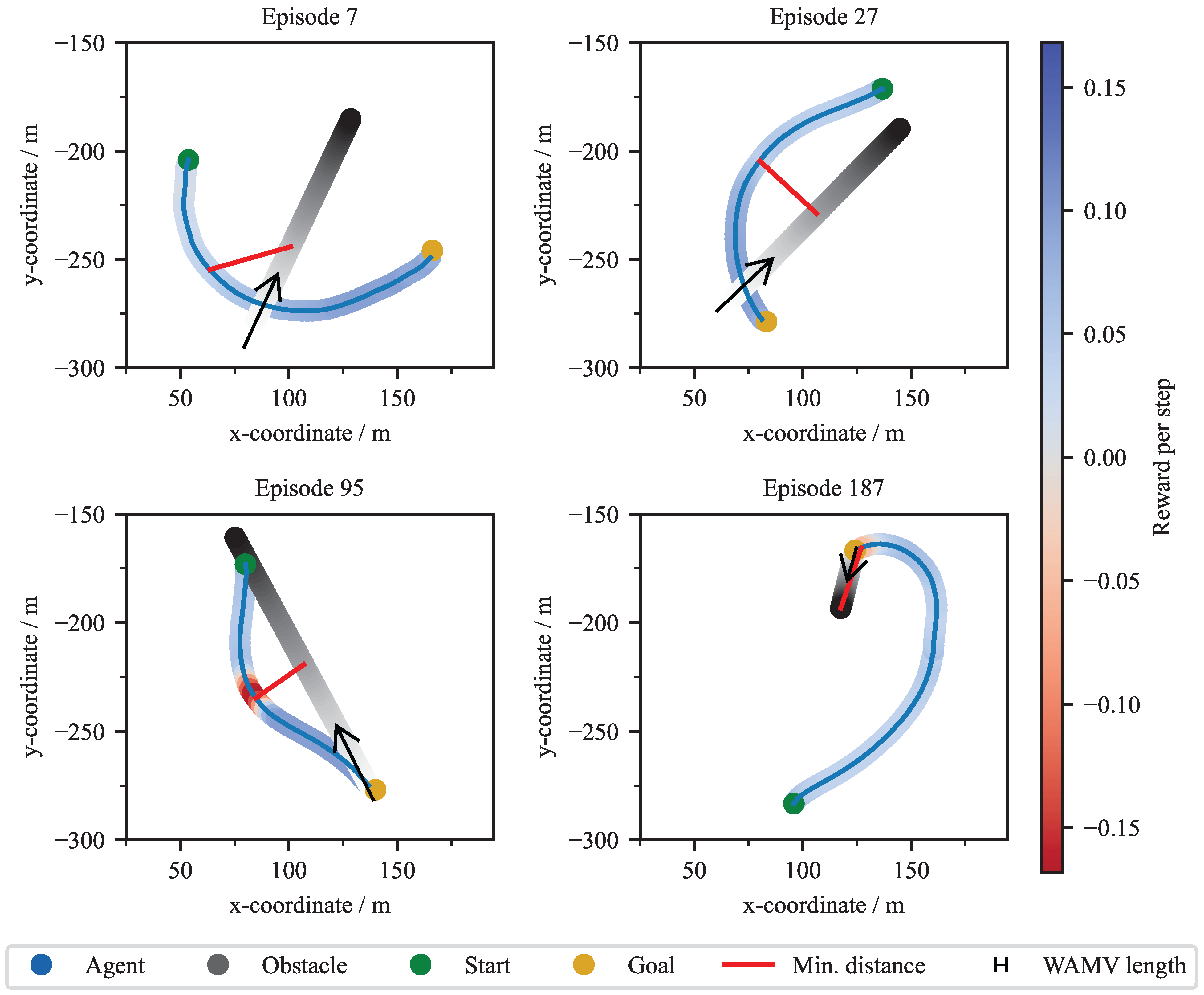
Figure 7 shows four exemplary trajectories from the validation simulations of one exemplary agent (C_1_3 agent). Each plot illustrates the agent’s path from a start to a goal position in environments with one to three static obstacles. The trajectories demonstrate that the agent successfully learned to maneuver around the obstacles. In the episodes shown, a collision can be observed because, unlike other agents, the agent does not manage to remain collision-free. Notably, even when a gap exists, the agent often chooses a wider path around a group of obstacles rather than navigating between them. The trajectory is color-coded to represent the reward at each timestep: blue segments signify positive rewards for efficient progress toward the target, while red segments indicate penalties incurred for close proximity to obstacles. When the agent gets close to the static obstacles, the reward is colored red accordingly, but this seems to be a reasonable compromise for quickly reaching the target position. Statistical validation results for the CA1 scenario are summarized in

Table 2. CA1: Statistical validation results for multiple agent parameterizations.

Name	Target Reached %	Collision %	Step Limit Reached %	Exited Workspace %
C_1_1	92.0	8.0	0.0	0.0
C_2_1	99.5	0.0	0.5	0.0
C_3_1	51.0	0.0	44.5	4.5
C_1_2	100.0	0.0	0.0	0.0
C_2_2	67.5	0.0	30.5	2.0
C_3_2	22.0	0.0	0.0	78.0
C_1_3	86.5	5.5	8.0	0.0
C_2_3	99.0	0.0	1.0	0.0
C_3_3	89.0	0.0	10.5	0.5
C_2_1_D1	98.5	0.0	0.0	1.5
C_2_1_D2	100.0	0.0	0.0	0.0

. Each agent was evaluated based on four key metrics: percentage of successful target reaching, percentage of episodes terminated due to step limit, percentage of collisions with the dynamic obstacle, and percentage of episodes in which the agent exited the defined workspace. It can be observed that certain parameter configurations lead to significantly lower target-reaching rates. Specifically, combinations with a relatively high obstacle avoidance reward ${\gamma }_{\mathrm{CA},\mathrm{OA}}$ compared to the target course reward ${\gamma }_{\mathrm{CA},\mathrm{TC}}$ tend to result in reduced performance (e.g., C_3_1 and C_3_2 agents). The primary cause of unsuccessful episodes is typically that the step limit is exceeded, indicating that the agent fails to reach the target within the allowed time. Notably, the configuration C_3_2 also frequently exits the workspace, indicating that the agent performs excessive evasive maneuvers.

To further evaluate the robustness of the agent, the parameter configuration C_2_1 was subjected to validation under disturbance conditions C_2_1_D1. It still shows high target achievement rates, even though it has not been trained with wind and waves previously. This indicates that the agent has learned to control the system dynamics sufficiently well to ensure safe navigation of the WAMV, even under previously unseen disturbances. However, the target was not achieved in 1.5% of the evaluation episodes, because the workspace was left. In contrast to this, agent C_2_1_D2 was trained with additional training under disturbances. After completion of training in 800 episodes without disturbances, this configuration was retrained with 400 episodes with disturbances. It shows a 100% target achievement rate; this implies that gradually increasing the complexity of the scenario and thus performing curriculum learning is beneficial for the agent’s training success, although in this scenario, the gains in success rate are rather small. These findings highlight the importance of a balanced reward formulation to ensure both efficient navigation and reliable target reaching in static obstacle environments.

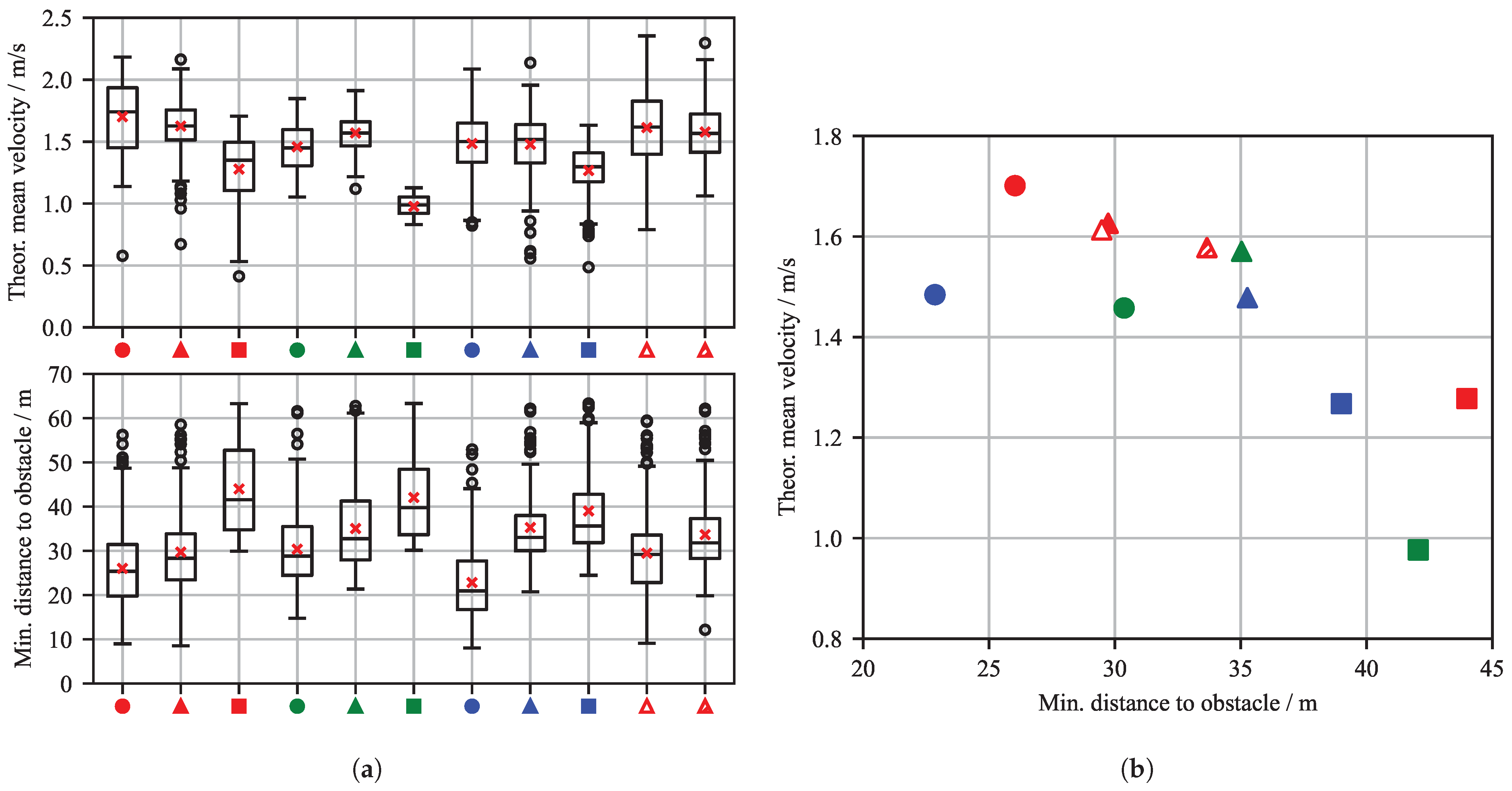
Figure 8a shows box plots with statistical data for the theoretical mean velocity and minimum distance to obstacles in the validation episodes in which the target was reached. For each successful episode, two metrics are evaluated: the minimum distance to the obstacle and the theoretical mean velocity of the WAMV. The minimum distance to obstacles refers to the closest point between the WAMV and the obstacle during the episode. The theoretical mean velocity is calculated as the straight-line distance between the start and target positions divided by the time the agent takes to reach the target position. The mean value across all validation episodes is marked with a red cross. The variation in CA1 configurations generally shows that agents with a higher parameter value for obstacle avoidance ${\gamma }_{\mathrm{CA},\mathrm{OA}}$ maintain a greater distance from obstacles. This corresponds to intuition in the design of parameter weighting. Furthermore, the theoretical mean speed decreases noticeably under these configurations. It becomes clear that there is a spread in the values of the evaluation metrics considered across the evaluation episodes, i.e., the agent does not always keep exactly the same distance from the varying number of static obstacles, but rather makes compromises in order to reach its goal quickly.

This is also consistent with the observations in the trajectories presented above (see Figure 7), where the agent maintains different distances to the obstacles. Now it also becomes apparent that the configuration that was subjected to disturbances in the evaluation, without having been trained with them C_2_1_D1 exhibits increased variance in velocity and minimum obstacle distance despite having good target reaching rates. In comparison to C_2_1, the standard deviation in the velocity of C_2_1_D1 increased from $0.23\mathrm{m}/\mathrm{s}$ to $0.29\mathrm{m}/\mathrm{s}$, and the standard deviation in the minimum obstacle distance increased from $9.03\mathrm{m}$ to $9.67\mathrm{m}$. In contrast, agent C_2_1_D2 shows significantly less dispersion, indicating that the additional training with 400 disturbance episodes has been clearly successful. The standard deviation in its velocity is $0.23\mathrm{m}/\mathrm{s}$ while the standard deviation in its minimum obstacle distance is $8.23\mathrm{m}$. The mean values and standard deviations of all agents are listed in Appendix A within

Table A3. Mean and standard deviation (SD) of the theoretical mean velocity and minimum obstacle distance for all agent parameterizations.

CA1	C_1_1	C_2_1	C_3_1	C_1_2	C_2_2	C_3_2	C_1_3	C_2_3	C_3_3	C_2_1_D1	C_2_1_D2
Mean of theor. mean velocity/m/s	1.70	1.63	1.28	1.46	1.57	0.98	1.48	1.48	1.27	1.61	1.58
SD of theor. mean velocity/m/s	0.27	0.23	0.29	0.19	0.16	0.08	0.24	0.26	0.19	0.29	0.23
Mean of min. obstacle distance/m	26.03	29.73	43.99	30.36	35.04	42.06	22.85	35.26	39,00	29.73	33.66
SD of min. obstacle distance/m	10.09	9.03	10.48	9.11	9.61	9.71	9.05	7.77	9.46	9.67	8.28
CA2	C_1_1	C_2_1	C_3_1	C_1_2	C_2_2	C_3_2	C_1_3	C_2_3	C_3_3	C_1_3_D1	C_1_3_D2
Mean of theor. mean velocity/m/s	1.85	1.56	1.37	1.72	1.67	1.44	1.80	1.62	1.28	1.70	1.72
SD of theor. mean velocity/m/s	0.28	0.14	0.20	0.18	0.30	0.22	0.25	0.17	0.19	0.37	0.35
Mean of min. obstacle distance/m	26.52	39.64	49.91	30.55	40.09	47.81	27.89	37.90	45.83	29.18	29.47
SD of min. obstacle distance/m	7.02	4.03	5.60	7.71	7.03	5.16	8.04	4.10	6.20	10.45	9.49
CA3	C_1_1	C_2_1	C_3_1	C_1_2	C_2_2	C_3_2	C_1_3	C_2_3	C_3_3	C_2_1_D1	C_2_1_D2
Mean of theor. mean velocity/m/s	1.40	1.22	0.67	1.19	1.00	0.96	1.01	0.73	0.85	1.08	0.99
SD of theor. mean velocity/m/s	0.23	0.19	0.13	0.21	0.14	0.21	0.39	0.13	0.18	0.32	0.23
Mean of min. obstacle distance/m	23.09	28.87	44.16	27.33	37.45	36.64	25.04	35.42	33.08	29.16	33.98
SD of min. obstacle distance/m	8.30	9.40	11.84	9.34	9.83	11.74	9.54	11.47	10.96	12.65	11.72

.

Figure 8b presents a scatter plot illustrating the theoretical mean velocity of the agents plotted against the minimum distance to the nearest static obstacle, across the considered reward and disturbance configurations. The plot reveals a clear trade-off between navigation speed and obstacle proximity: higher velocities tend to correlate with reduced minimum distances, necessitating a compromise between short target reaching time and safety. This compromise also reflects natural expectations regarding the influence of the parameters, but helps to quantify this impact. Given the approximate length of the WAMV platform ($5\mathrm{m}$), all observed minimum distances are sufficiently large to avoid collisions, indicating that the agents maintain safe margins even at higher speeds. Figure 8b also highlights the influence of reward shaping on agent behavior: Configurations with stronger emphasis on obstacle avoidance tend to maintain larger safety distances but may sacrifice speed, whereas those prioritizing target course alignment may achieve faster trajectories at the cost of reduced clearance. These insights are critical for tuning reward functions in real-world applications where both safety and efficiency are paramount.

3.2. Scenario CA2—Dynamic Obstacle Avoidance

In the CA2 scenario, the agent is trained and evaluated in a dynamic collision avoidance task involving a single moving obstacle. The scenario is described in detail in Section 2.2.4. To investigate the influence of reward design on agent behavior, the same variations in reward weights ${\gamma }_{\mathrm{CA},\mathrm{OA}}$ (obstacle avoidance) and ${\gamma }_{\mathrm{CA},\mathrm{TC}}$ as in CA1 (target course) are considered; see Table 1. Furthermore, multiple disturbance configurations are evaluated to assess the robustness of the learned policy. In addition to the trajectory plots already presented in Figure 7, Figure 9 also contains the trajectories of the obstacle ship, as well as the minimum distances to the dynamic obstacle marked in red. The gray curve represents the trajectory of the dynamic obstacle, where lighter segments denote earlier positions in time. The direction of the black arrow corresponds to the direction of movement of the obstacle. The agent with the configuration C_1_3 managed to avoid a collision in all four test episodes.

Notably, in all shown cases, the WAMV consistently performs the avoidance maneuver to the right. This can be explained by the scenario setup, as the dynamic obstacle always comes head-on or from the right. In this case, the agent has learned that it can prevent most collisions by slightly evading to the right.

Table 3. CA2: Statistical validation results for multiple agent parameterizations.

Name	Target Reached %	Collision %	Step Limit Reached %	Exited Workspace %
C_1_1	98.5	0.0	1.5	0.0
C_2_1	100.0	0.0	0.0	0.0
C_3_1	100.0	0.0	0.0	0.0
C_1_2	100.0	0.0	0.0	0.0
C_2_2	100.0	0.0	0.0	0.0
C_3_2	99.5	0.5	0.0	0.0
C_1_3	100.0	0.0	0.0	0.0
C_2_3	100.0	0.0	0.0	0.0
C_3_3	99.0	0.0	1.0	0.0
C_1_3_D1	95.5	4.0	0.0	0.5
C_1_3_D2	98.5	1.5	0.0	0.0

summarizes the statistical validation results of the trained agents in the CA2 scenario. The same evaluation criteria are used across all test episodes: percentage of successful target reaching, percentage of episodes terminated due to step limit, percentage of collisions with the dynamic obstacle, and percentage of episodes in which the agent exited the defined workspace. Across all parameterizations, the agents demonstrate high reliability, with most achieving target-reaching rates above 98% without disturbances. Notably, the agent C_1_3 achieved a 100% target reaching rates, without any collisions, step limit violations, or workspace exits. Minor deviations are observed in agents such as C_1_1 and C_3_2, which exhibit slightly reduced target reaching rates and isolated cases of workspace exits or collisions. However, no trend can be identified that would allow conclusions to be drawn about the parameter configuration. Overall, the agents learned to avoid dynamic obstacles more effectively than static ones. This can probably be explained by the fact that, in CA1, obstacles usually block the path to the goal, necessitating evasive trajectories from the beginning. In contrast, CA2 has scenario variations in which agents can reach the goal without evading any obstacles.

To evaluate the robustness of the C_1_3 configuration, it is also tested under environmental disturbances C_1_3_D1, conditions it had not encountered during initial training. Under these disturbed conditions, the agent’s target achievement rate decreased. The collision rate increased to $4.0\%$, and the agent exited the workspace in $0.5\%$ of the episodes. To improve performance, the agent was retrained for an additional 400 episodes C_1_3_D2 with these disturbances present. This retrained configuration achieved a target-reaching rate of $98.5\%$, a notable improvement. This result suggests that curriculum learning, a gradual increase in scenario complexity, enhances the agent’s performance. However, collisions still occurred in $1.5\%$ of cases. For comparison, we also trained agents with disturbances present from the beginning of the training. This approach yielded substantially poorer performance and was therefore not pursued further.

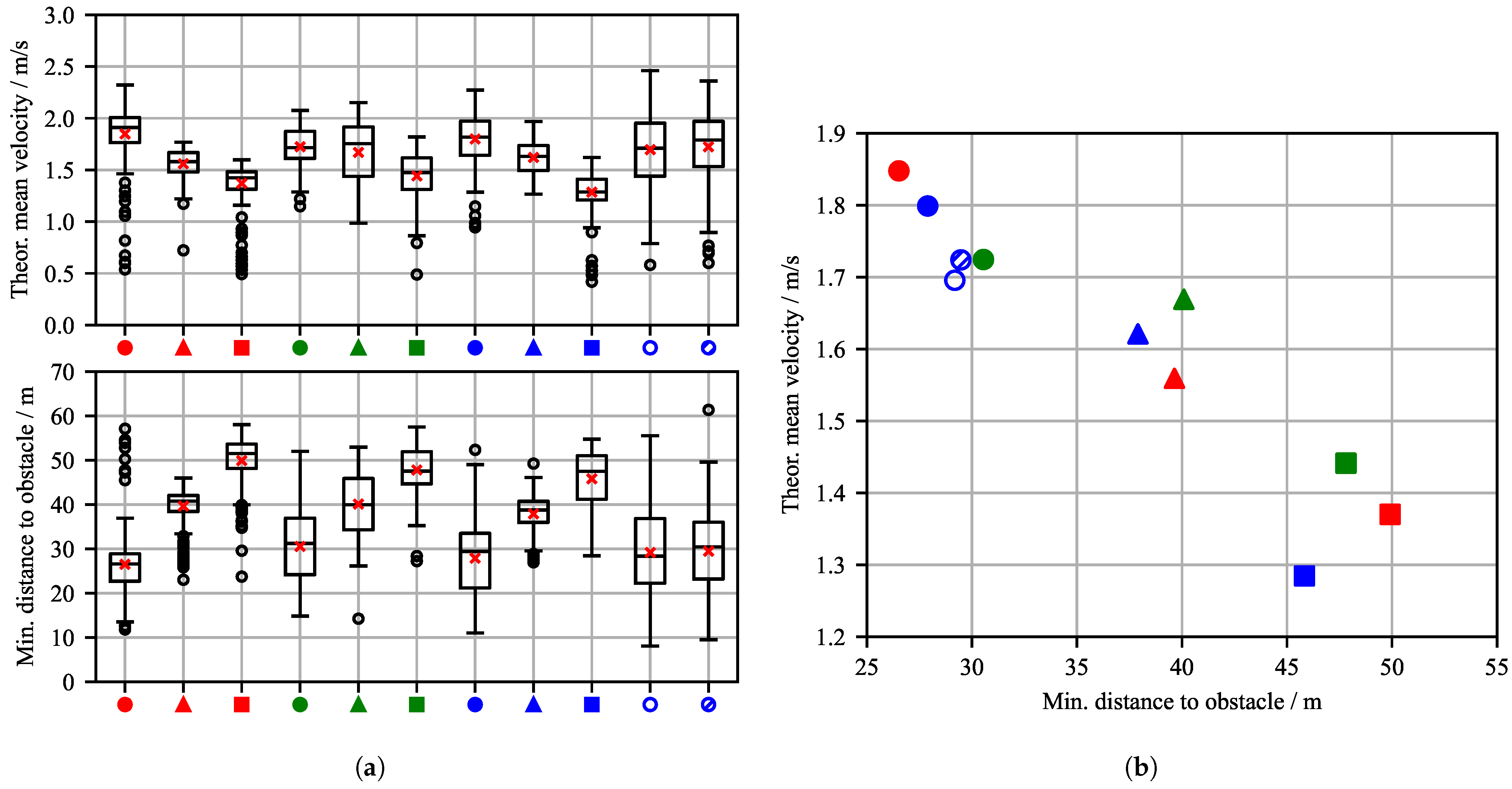
Figure 10a presents box plots of the theoretical mean velocity and minimum obstacle distance from the CA2 evaluation episodes. Similar to the CA1 scenario, these results reveal a clear dependency on the reward function parameters. Increasing the obstacle avoidance weight, ${\gamma }_{\mathrm{CA},\mathrm{OA}}$ (indicated by symbol shape), results in more cautious agent behavior. Consequently, the agent maintains a greater distance from the obstacle, which increases the theoretical mean velocity to reach the target position. In contrast, increasing the target course weight, ${\gamma }_{\mathrm{CA},\mathrm{TC}}$ (indicated by color), does not significantly influence the mean values for velocity or distance. However, a larger parameter value generally correlates with a greater spread in both metrics. Both agents tested under environment disturbance conditions, C_1_3_D1 and C_1_3_D2, show a marginally higher data dispersion in their results without a statistically significant difference between them.

Theoretical mean velocity and minimum distance to obstacles are plotted against each other in a scatter diagram (see Figure 10b). The results reveal a trade-off between minimum obstacle distance and theoretical mean speed: The closer the WAMV passes by the obstacle, the faster it moves to the goal. Considering the approximate length of the WAMV, which is about $5\mathrm{m}$, all depicted minimum distances can be considered as non-critical. The mean minimum distances to the dynamic obstacle vary between $26\mathrm{m}$ and $50\mathrm{m}$.

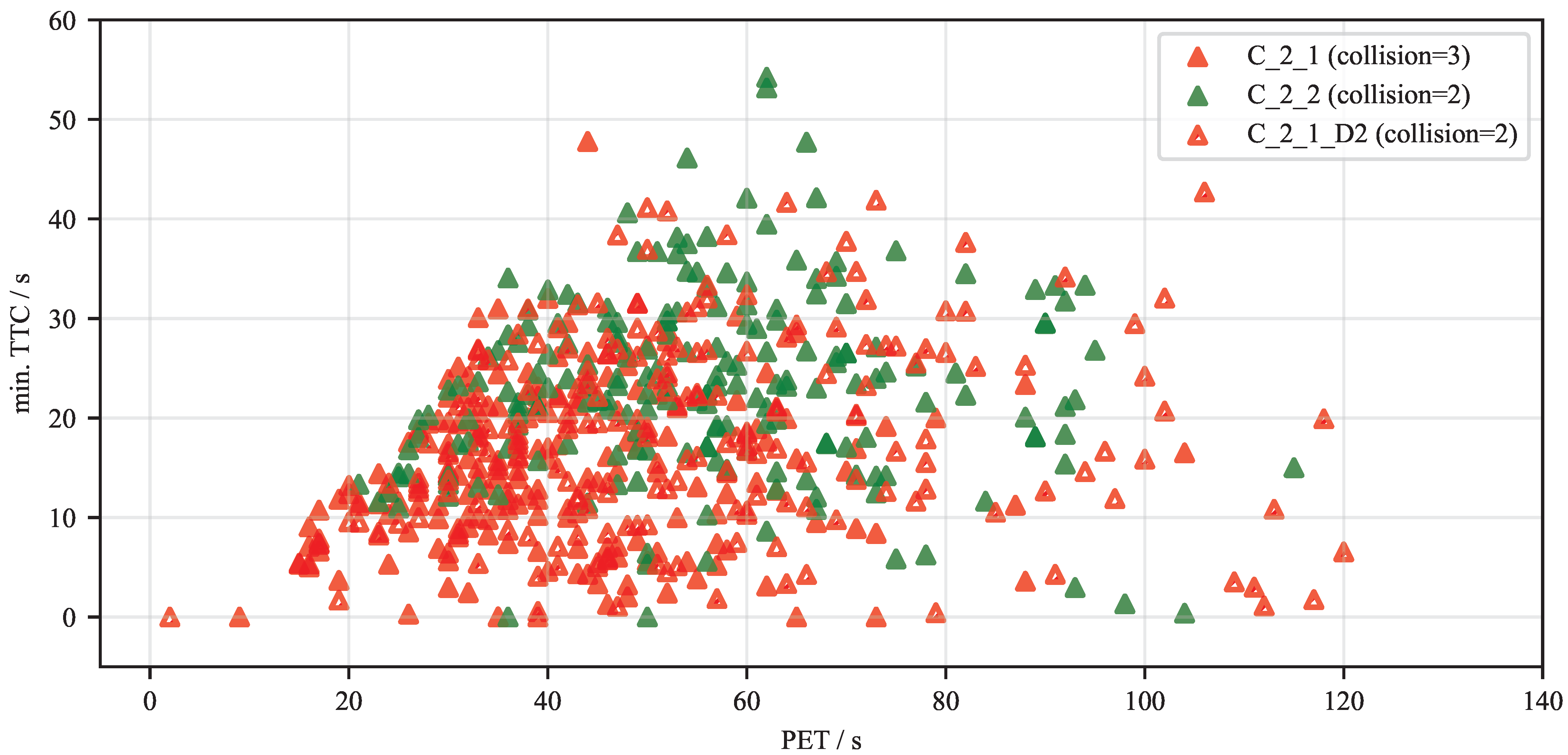
To further analyze the safety performance of the trained agents in dynamic encounters, Figure 11 presents a scatter plot of the minimum TTC against the PET for three distinct agent configurations. These metrics are critical for quantifying the risk associated with each encounter, where lower values indicate a higher collision risk.

Agents C_1_3 and C_2_1, which were neither trained nor validated with environmental disturbances, demonstrate robustly safe behavior. Their encounters predominantly populate regions of higher TTC and PET values, and neither agent registered a collision during the 200 validation episodes. A subtle difference is observable between them, as C_1_3 generally operates with lower TTC values compared to C_2_1. In contrast, the agent C_1_3_D2, which underwent additional training with disturbances and was validated under the same conditions, exhibits a notable shift in its operational characteristics. Its data points are more densely clustered in the lower-left quadrant of the plot, with a visible shift towards lower PET values, indicating that the agent struggles to maintain large safety margins when subjected to environmental disturbances. This performance degradation is further evidenced by the three collisions this agent experienced during validation. The results highlight a clear challenge in achieving robustness; while the agent learns to operate in disturbed conditions, it does so with a reduced safety envelope, revealing a difficult trade-off between operational capability and consistent collision avoidance.

In summary, the proposed formulation for the reinforcement learning agents enables effective collision avoidance not only with static obstacles but also in scenarios involving dynamically moving obstacles. It is important to critically note that, in some cases, avoiding collisions with dynamic obstacles may be easier to achieve than with static ones. In static scenarios, there is almost always at least one obstacle directly in the direct path of the vessel. In contrast, the defined dynamic obstacle avoidance setup includes scenario variations where evasive maneuvers were not strictly necessary to prevent a collision. This is also reflected in the training outcomes: success rates in dynamic obstacle avoidance are consistently high, and preliminary experiments indicate that pre-training without obstacles would not have been required to achieve reliable performances. Next, combined scenarios involving both static and dynamic obstacles are considered. These represent a fusion of CA1 and CA2 and are designed to closely approximate real-world conditions.

3.3. Scenario CA3—Multi-Hindrance Scenario

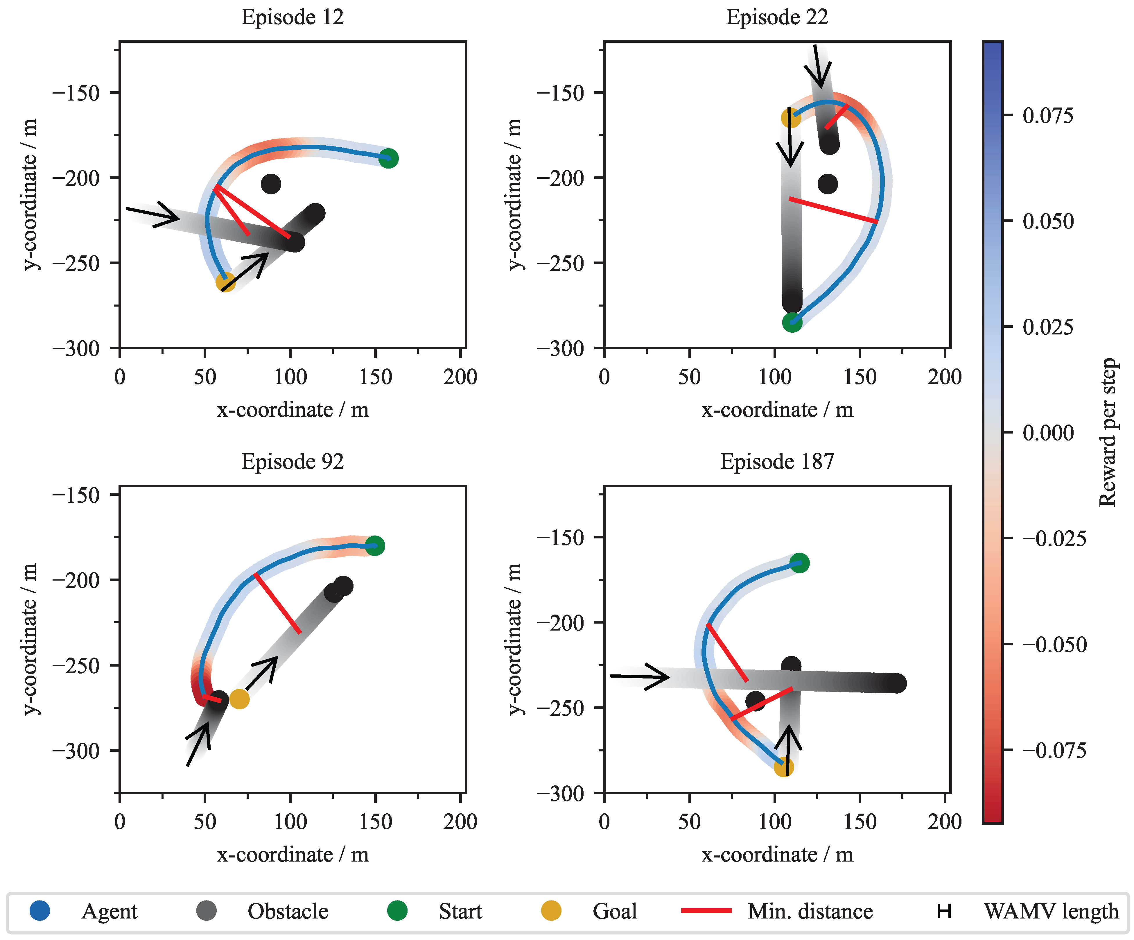
The final scenario, CA3, assesses the agent’s performance in a complex multi-hindrance environment combining both static and dynamic obstacles, as described in Section 2.2.4. Exemplary validation trajectories for the C_1_1 agent are depicted in Figure 12. These plots illustrate the agent’s capacity to navigate complex encounters. The agent successfully develops avoidance strategies, such as crossing behind the path of dynamic obstacles (Episode 12 and 92) or navigating between them (Episode 22). The red connecting lines mark the minimum distance between the WAMV and the respective dynamic objects. The direction of the black arrow corresponds to the direction of movement of the obstacle. This scenario’s difficulty is also highlighted by Episode 187, which terminates in a collision with a dynamic obstacle.

A statistical summary of the performance across all reward configurations is provided in

Table 4. CA3: Statistical validation results for multiple agent parameterizations.

Name	Target Reached %	Collision %	Step Limit Reached %	Exited Workspace %
C_1_1	95.0	5.0	0.0	0.0
C_2_1	98.0	1.5	0.5	0.0
C_3_1	96.0	0.0	4.0	0.0
C_1_2	97.5	2.5	0.0	0.0
C_2_2	99.0	1.0	0.0	0.0
C_3_2	97.0	2.0	1.0	0.0
C_1_3	94.5	5.0	0.5	0.0
C_2_3	93.0	7.0	0.0	0.0
C_3_3	96.5	2.5	1.0	0.0
C_2_1_D1	91.0	8.5	0.0	0.5
C_2_1_D2	98.5	1.0	0.0	0.5

. Due to the increased scenario complexity, overall success rates are slightly lower and more variable than in the single-obstacle scenarios. Target-reaching rates for agents trained without disturbances remained high, generally between $93.0\%$ (C_2_3) and $99.0\%$ (C_2_2). Unlike the static-only CA1 scenario, failure was not dominated by workspace violations or time-outs, which were minimal across all configurations. Instead, the primary failure mode was direct collision, with rates ranging from $0.0\%$ (C_3_1) to $7.0\%$ (C_2_3).

The impact of environmental disturbances is significant. The C_2_1_D1 agent, which was validated under disturbances without prior training, experienced a substantial performance drop: its success rate fell from $98.0\%$ to $91.0\%$, while its collision rate increased from $1.5\%$ to $8.5\%$. In contrast, the C_2_1_D2 agent, which underwent an additional 400 episodes of curriculum learning with disturbances, demonstrated robustness. This agent restored its target-reaching success rate to $98.5\%$ and reduced its collision rate to $1.0\%$, performing comparably to the original agent in ideal conditions. This result strongly validates the curriculum learning approach, where scenario complexity is gradually increased to achieve robust policy generalization.

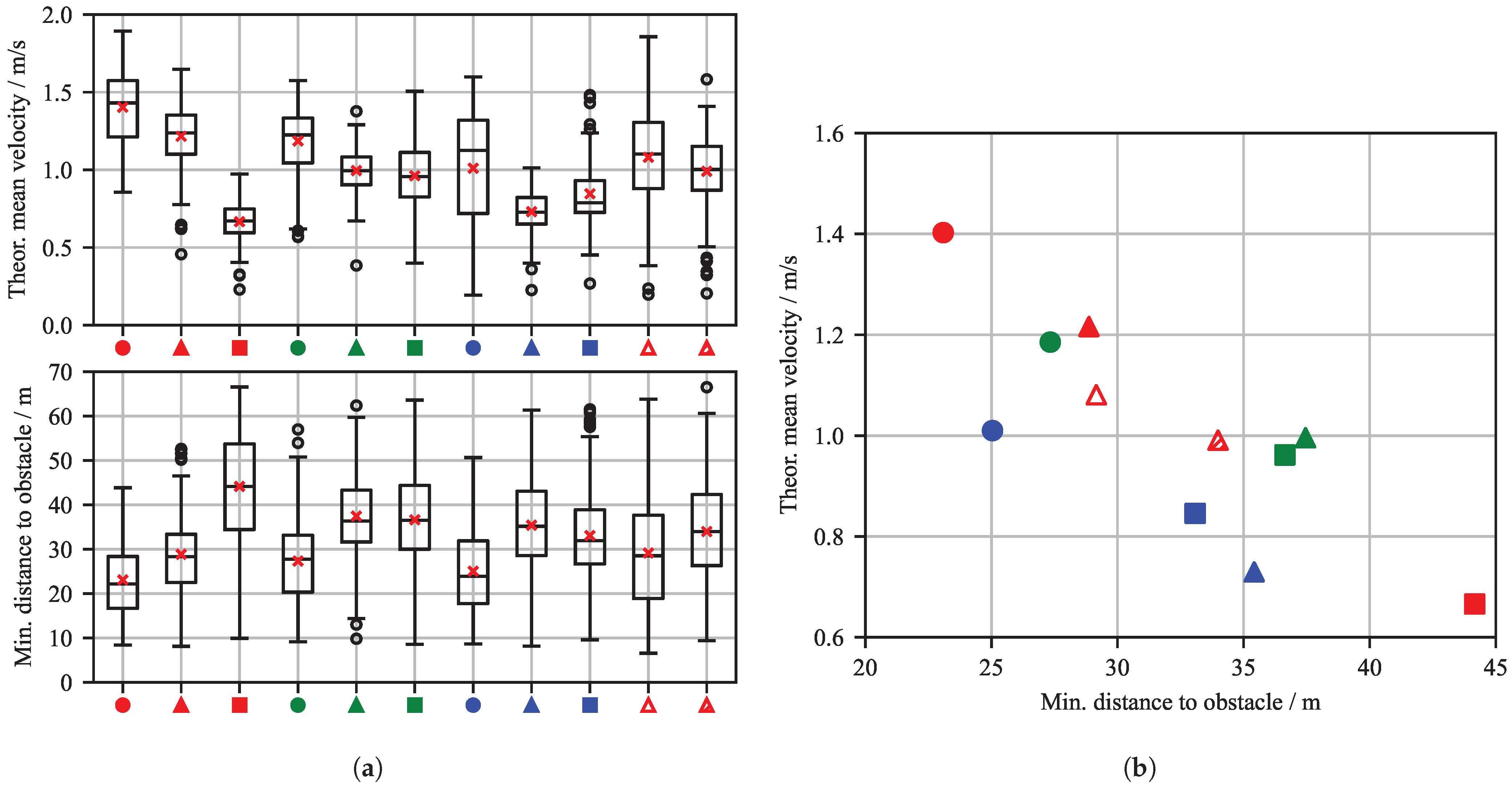
The trade-off between mission efficiency and safety margins is quantitatively mapped in Figure 13. The box plots in Figure 13a confirm the influence of the reward shaping parameters. Agents with a higher obstacle avoidance weight ${\gamma }_{\mathrm{CA},\mathrm{OA}}$ (e.g., C_3_1, C_3_3) consistently maintain a larger minimum distance to obstacles, adopting a more cautious policy. The scatter plot in Figure 13b visualizes this compromise directly. An inverse relationship exists between navigation speed and safety clearance. For instance, the C_1_1 agent achieves a high mean velocity of $1.4\mathrm{m}/\mathrm{s}$ but maintains a tighter average distance of approximately $23\mathrm{m}$. Conversely, the highly cautious C_3_1 agent achieves a large $44\mathrm{m}$ minimum distance at the cost of a significantly reduced mean velocity of only $0.67\mathrm{m}/\mathrm{s}$. Figure 13a also reinforces the disturbance training findings: the C_2_1_D1 agent (unfilled triangle) exhibits high variance in both velocity, with a standard deviation of $0.32\mathrm{m}/\mathrm{s}$, and distance, with a standard deviation of $12.65\mathrm{m}$. In contrast, the retrained C_2_1_D2 agent (hatched triangle) shows a much more consistent and stable performance. Its standard deviations are $0.23\mathrm{m}/\mathrm{s}$ for velocity and $11.72\mathrm{m}$ for minimum obstacle distance. This is similar to the baseline C_2_1, which shows standard deviations of $0.19\mathrm{m}/\mathrm{s}$ and $9.4\mathrm{m}$, respectively.

To further analyze the safety characteristics of the agents in the multi-hindrance scenario, Figure 14 plots the minimum TTC against the PET for three configurations. This analysis reveals nuanced differences in their avoidance behaviors. The C_2_2 agent, for instance, generally exhibits higher PET values compared to the other agents, indicating that its policy favors maneuvers that create greater temporal separation from obstacles, even at the cost of accepting a wide range of TTCs.

In contrast, the agent trained with disturbances, C_2_1_D2, displays a significantly higher variance in both its TTC and PET values. This increased scatter suggests that while the agent can still operate effectively, the environmental disturbances introduce a degree of unpredictability, making it more difficult to maintain consistent safety margins. The most critical encounters are represented by data points where the TTC approaches zero. These instances correspond directly to the recorded collisions—three for C_2_1, two for C_2_2, and two for C_2_1_D2—as well as other high-risk, near-miss situations, underscoring the residual risk present even in well-trained policies when faced with complex, dynamic scenarios.

4. Conclusions

This work presents a reinforcement learning-based framework for autonomous maritime maneuvering, with a particular focus on collision avoidance in static and dynamic environments. It is re-emphasized that the primary objective of this work was not to benchmark DRL against other control paradigms (e.g., MPC, DWA), but rather to perform a systematic analysis of the behavioral variability of a single RL formulation under different reward parameterizations. Although a direct numerical comparison would go beyond the scope of this article, this section provides a comparative discussion of the expected strengths and weaknesses. For instance, a well-tuned MPC utilizing a ship model would perform well in explicit constraint handling and optimal control, given an accurate model. However, its performance is heavily reliant on that model’s accuracy and the calibration of its cost function weights—a tuning challenge analogous to the reward shaping we investigate here. Similarly, classical methods like the DWA are computationally efficient but can be prone to local minima and may produce non-optimal or jerky maneuvers in complex, multi-obstacle scenarios. In contrast, the DRL agent, once trained, learns to generate trajectories that implicitly balance competing objectives over a long horizon, often with greater robustness to unmodeled disturbances.

The proposed framework includes a modular simulation and training architecture, allowing for automated training and evaluation of agents across randomized scenario configurations. The scenario definitions within the simulation environment, ranging from static to dynamic to combined obstacle avoidance scenarios, support diverse and efficient training conditions. The use of randomized obstacle placements and disturbance conditions further enhances the generalizability of the learned policies.

Across all scenarios, agents demonstrated high reliability in reaching target destinations while avoiding collisions. In particular, the CA2 scenario involving dynamic obstacles yielded consistently high success rates, with agents maintaining safe distances and efficient trajectories. The CA1 scenario revealed that certain reward configurations—especially those with disproportionate emphasis on target course alignment—can lead to suboptimal behavior, such as excessive evasive maneuvers or failure to reach the goal within the step limit. These findings underscore the importance of balanced reward shaping.

The multi-hindrance CA3 scenario, which integrated both static and dynamic elements, provided the most comprehensive test of the agents’ capabilities. Despite this complexity, agents trained with balanced reward weights achieved high target-reaching rates, often exceeding $98\%$. This scenario highlighted the critical impact of environmental disturbances; the baseline agent’s performance degraded significantly under these conditions, with collision rates increasing to $8.5\%$. However, the successful application of curriculum learning—retraining the agent with disturbances included—restored the success rate to $98.5\%$ and reduced collisions to $1.0\%$. This finding powerfully demonstrates that a gradual increase in scenario complexity is an effective strategy for achieving robust policy generalization in complex, dynamic environments.

A key contribution of this work lies in the structured evaluation of reward parameterizations. By varying the weights of obstacle avoidance and target course terms, the study provides insights into the trade-offs between safety, efficiency, and robustness. The resulting scatter plots and statistical analyses offer a quantitative basis for selecting reward configurations that align with specific operational priorities.

In addition to the parameter study, the framework itself represents a contribution. The integration of ROS, VRX, and Stable Baselines3 enables scalable and reproducible training of RL agents in maritime environments. The automated training pipeline and scenario generation tools facilitate rapid experimentation and support future extensions.

Overall, this work provides a foundation for systematic RL-based control development in maritime robotics, emphasizing transparency, reproducibility, and scenario-driven evaluation. Furthermore, the framework created can be used in the future to develop even more detailed scenarios and create a greater variety of scenarios. For example, additional encounter situations may be defined. Based on this, the trained agents can be validated in reality. Based on the literature review, the most commonly encountered situations were selected, and the focus was placed on scenario variability. In detail, randomized variations are carried out within a defined scenario, for example, a head-on encounter. The framework is to be further formalized in order to achieve transferability to other use cases and to facilitate scenario-based training. Another possibility is to use RL agents to develop other control approaches. For example, the partially unpredictable behavior of agents could be used to test an MPC. While the current study focuses on a single RL formulation, future work will explore comparisons with alternative control strategies, such as MPC or hybrid approaches. Moreover, the integration of COLREG into the reward function is planned to further align agent behavior with real-world operational standards. This includes integrating compliance directly into the reward function via reward shaping (i.e., adding a penalty for non-compliant maneuvers), using action masking to proactively prevent the agent from selecting a non-compliant maneuver. In the future, RL agents are planned to be used on embedded systems to perform tests on research boats, for which the framework needs to be switched to LExCI. The LExCI framework enables users to apply RL to real-world engineering problems on professional hardware [66]. If the RL agent continues to be used for automated driving, safety-related aspects must also be considered. In this context, Bedei et al. [67] show promising approaches that can be explored.

References

1. de Andrade, E.M.; Sales, J.S.; Fernandes, A.C. Operative Unmanned Surface Vessels (USVs): A Review of Market-Ready Solutions. Automation 2025, 6, 17. [Google Scholar] [CrossRef]
2. Bai, X.; Li, B.; Xu, X.; Xiao, Y. A Review of Current Research and Advances in Unmanned Surface Vehicles. J. Mar. Sci. Appl. 2022, 21, 47–58. [Google Scholar] [CrossRef]
3. Chen, Z.; Bao, T.; Zhang, B.; Wu, T.; Chu, X.; Zhou, Z. Deep Reinforcement Learning Methods for USV Control: A Review. In Proceedings of the 2023 China Automation Congress (CAC), Chongqing, China, 17–19 November 2023; pp. 1526–1531. [Google Scholar] [CrossRef]
4. Liu, Z.; Zhang, Y.; Yu, X.; Yuan, C. Unmanned surface vehicles: An overview of developments and challenges. Annu. Rev. Control 2016, 41, 71–93. [Google Scholar] [CrossRef]
5. Xue, J.; Yang, P.; Li, Q.; Song, Y.; Gelder, P.H.A.J.M.v.; Papadimitriou, E.; Hu, H. Machine Learning in Maritime Safety for Autonomous Shipping: A Bibliometric Review and Future Trends. J. Mar. Sci. Eng. 2025, 13, 746. [Google Scholar] [CrossRef]
6. Ibrahim, S.; Mostafa, M.; Jnadi, A.; Salloum, H.; Osinenko, P. Comprehensive Overview of Reward Engineering and Shaping in Advancing Reinforcement Learning Applications. arXiv 2024, arXiv:2408.10215. [Google Scholar] [CrossRef]
7. Yu, R.; Wan, S.; Wang, Y.; Gao, C.X.; Gan, L.; Zhang, Z.; Zhan, D.C. Reward Models in Deep Reinforcement Learning: A Survey. arXiv 2025, arXiv:2506.15421. [Google Scholar] [CrossRef]
8. Schumacher, M.; Adriano, C.M.; Giese, H. Challenges in Reward Design for Reinforcement Learning-based Traffic Signal Control: An Investigation using a CO2 Emission Objective. SUMO Conf. Proc. 2023, 4, 131–151. [Google Scholar] [CrossRef]
9. Zhang, W. Design of Reward Functions for Autonomous Driving Based on Reinforcement Learning: Balancing Safety and Efficiency. Appl. Comput. Eng. 2025, 146, 9–22. [Google Scholar] [CrossRef]
10. Osika, Z.; Zatarain-Salazar, J.; Oliehoek, F.A.; Murukannaiah, P.K. Navigating Trade-offs: Policy Summarization for Multi-Objective Reinforcement Learning. In ECAI 2024; IOS Press: Amsterdam, The Netherlands, 2024. [Google Scholar] [CrossRef]
11. Schulman, J.; Wolski, F.; Dhariwal, P.; Radford, A.; Klimov, O. Proximal Policy Optimization Algorithms. arXiv 2017, arXiv:1707.06347. [Google Scholar] [CrossRef]
12. Bingham, B.; Agüero, C.; McCarrin, M.; Klamo, J.; Malia, J.; Allen, K.; Lum, T.; Rawson, M.; Waqar, R. Toward Maritime Robotic Simulation in Gazebo. In Proceedings of the OCEANS 2019 MTS/IEEE SEATTLE, Seattle, WA, USA, 27–31 October 2019; pp. 1–10. [Google Scholar] [CrossRef]
13. Siciliano, B.; Khatib, O. (Eds.) Springer Handbook of Robotics; Springer: Berlin/Heidelberg, Germany, 2008. [Google Scholar] [CrossRef]
14. Chen, C.S.; Lin, C.J.; Lai, C.C.; Lin, S.Y. Velocity Estimation and Cost Map Generation for Dynamic Obstacle Avoidance of ROS Based AMR. Machines 2022, 10, 501. [Google Scholar] [CrossRef]
15. Ferguson, D.; Likhachev, M. Efficiently Using Cost Maps For Planning Complex Maneuvers. 2008. Available online: https://repository.upenn.edu/handle/20.500.14332/34770 (accessed on 1 July 2025).
16. Racinskis, P.; Arents, J.; Greitans, M. Constructing Maps for Autonomous Robotics: An Introductory Conceptual Overview. Electronics 2023, 12, 2925. [Google Scholar] [CrossRef]
17. Thrun, S. Robotic mapping: A survey. In Exploring Artificial Intelligence in the New Millennium; Morgan Kaufmann Publishers Inc.: San Francisco, CA, USA, 2003; pp. 1–35. [Google Scholar]
18. Yi, C.; Jeong, S.; Cho, J. Map Representation for Robots. Smart Comput. Rev. 2012, 2, 18–27. [Google Scholar] [CrossRef]
19. Macenski, S.; Moore, T.; Lu, D.V.; Merzlyakov, A.; Ferguson, M. From the desks of ROS maintainers: A survey of modern & capable mobile robotics algorithms in the robot operating system 2. Robot. Auton. Syst. 2023, 168, 104493. [Google Scholar] [CrossRef]
20. Sanchez, M.; Morales, J.; Martínez, J.; Fernández-Lozano, J.; Garcia, A. Automatically Annotated Dataset of a Ground Mobile Robot in Natural Environments via Gazebo Simulations. Sensors 2022, 22, 5599. [Google Scholar] [CrossRef] [PubMed]
21. Souissi, O.; Benatitallah, R.; Duvivier, D.; Artiba, A.; Belanger, N.; Feyzeau, P. Path planning: A 2013 survey. In Proceedings of the 2013 International Conference on Industrial Engineering and Systems Management (IESM), Rabat, Morocco, 28–30 October 2013; pp. 1–8. [Google Scholar]
22. LaValle, S.M. Planning Algorithms, reprinted ed.; Cambridge University Press: New York, NY, USA, 2014. [Google Scholar]
23. Karaman, S.; Frazzoli, E. Sampling-based algorithms for optimal motion planning. Int. J. Robot. Res. 2011, 30, 846–894. [Google Scholar] [CrossRef]
24. Loe, Ø. Collision Avoidance Concepts for Marine Surface Craft. Trondheim 2007, 19, 111. [Google Scholar]
25. Seder, M.; Petrovic, I. Dynamic window based approach to mobile robot motion control in the presence of moving obstacles. In Proceedings of the 2007 IEEE International Conference on Robotics and Automation, Rome, Italy, 10–14 April 2007; pp. 1986–1991. [Google Scholar] [CrossRef]
26. Heiberg, A.; Larsen, T.N.; Meyer, E.; Rasheed, A.; San, O.; Varagnolo, D. Risk-based implementation of COLREGs for autonomous surface vehicles using deep reinforcement learning. Neural Netw. 2022, 152, 17–33. [Google Scholar] [CrossRef]
27. Vagale, A.; Oucheikh, R.; Bye, R.T.; Osen, O.L.; Fossen, T.I. Path planning and collision avoidance for autonomous surface vehicles I: A review. J. Mar. Sci. Technol. 2021, 26, 1292–1306. [Google Scholar] [CrossRef]
28. Lamini, C.; Benhlima, S.; Elbekri, A. Genetic Algorithm Based Approach for Autonomous Mobile Robot Path Planning. Procedia Comput. Sci. 2018, 127, 180–189. [Google Scholar] [CrossRef]
29. Wang, D.; Tan, D.; Liu, L. Particle swarm optimization algorithm: An overview. Soft Comput. 2018, 22, 387–408. [Google Scholar] [CrossRef]
30. Contreras-Cruz, M.A.; Ayala-Ramirez, V.; Hernandez-Belmonte, U.H. Mobile robot path planning using artificial bee colony and evolutionary programming. Appl. Soft Comput. 2015, 30, 319–328. [Google Scholar] [CrossRef]
31. Zhou, Y.; Tuzel, O. VoxelNet: End-to-End Learning for Point Cloud Based 3D Object Detection. In Proceedings of the 2018 IEEE/CVF Conference on Computer Vision and Pattern Recognition, Salt Lake City, UT, USA, 18–22 June 2018; pp. 4490–4499. [Google Scholar] [CrossRef]
32. Campbell, S.; Naeem, W.; Irwin, G.W. A review on improving the autonomy of unmanned surface vehicles through intelligent collision avoidance manoeuvres. Annu. Rev. Control 2012, 36, 267–283. [Google Scholar] [CrossRef]
33. Tsardoulias, E.; Iliakopoulou, K.; Kargakos, A.; Petrou, L. A Review of Global Path Planning Methods for Occupancy Grid Maps Regardless of Obstacle Density. J. Intell. Robot. Syst. 2016, 84, 829–858. [Google Scholar] [CrossRef]
34. Xing, B.; Yu, M.; Liu, Z.; Tan, Y.; Sun, Y.; Li, B. A Review of Path Planning for Unmanned Surface Vehicles. J. Mar. Sci. Eng. 2023, 11, 1556. [Google Scholar] [CrossRef]
35. Chu, Y.; Gao, Q.; Yue, Y.; Lim, E.G.; Paoletti, P.; Ma, J.; Zhu, X. Evolution of Unmanned Surface Vehicle Path Planning: A Comprehensive Review of Basic, Responsive, and Advanced Strategic Pathfinders. Drones 2024, 8, 540. [Google Scholar] [CrossRef]
36. Alessandretti, A.; Aguiar, A.P.; Jones, C.N. Trajectory-tracking and path-following controllers for constrained underactuated vehicles using Model Predictive Control. In Proceedings of the 2013 European Control Conference (ECC), Zurich, Switzerland, 17–19 July 2013; pp. 1371–1376. [Google Scholar] [CrossRef]
37. Thyri, E.H.; Breivik, M. Collision avoidance for ASVs through trajectory planning: MPC with COLREGs-compliant nonlinear constraints. Model. Identif. Control Nor. Res. Bull. 2022, 43, 55–77. [Google Scholar] [CrossRef]
38. Kamel, M.S.; Stastny, T.; Alexis, K.; Siegwart, R. Model Predictive Control for Trajectory Tracking of Unmanned Aerial Vehicles Using Robot Operating System. In Robot Operating System (ROS). Studies in Computational Intelligence; Springer: Cham, Switzerland, 2017. [Google Scholar] [CrossRef]
39. Wallace, M.T.; Streetman, B.; Lessard, L. Model Predictive Planning: Trajectory Planning in Obstruction-Dense Environments for Low-Agility Aircraft. arXiv 2024, arXiv:2309.16024. [Google Scholar] [CrossRef]
40. Li, Z.; Sun, J. Disturbance Compensating Model Predictive Control With Application to Ship Heading Control. IEEE Trans. Control Syst. Technol. 2012, 20, 257–265. [Google Scholar] [CrossRef]
41. Moser, M.M.; Huang, M.; Abel, D. Model Predictive Control for Safe Path Following in Narrow Inland Waterways for Rudder Steered Inland Vessels*. In Proceedings of the 2023 European Control Conference (ECC), Bucharest, Romania, 13–16 June 2023; pp. 1–6. [Google Scholar] [CrossRef]
42. Wang, Y.; Tong, H.; Fu, M. Line-of-sight guidance law for path following of amphibious hovercrafts with big and time-varying sideslip compensation. Ocean. Eng. 2019, 172, 531–540. [Google Scholar] [CrossRef]
43. Fossen, T.I.; Breivik, M.; Skjetne, R. Line-of-sight path following of underactuated marine craft. IFAC Proc. Vol. 2003, 36, 211–216. [Google Scholar] [CrossRef]
44. Perez, A.; Platt, R.; Konidaris, G.; Kaelbling, L.; Lozano-Perez, T. LQR-RRT*: Optimal sampling-based motion planning with automatically derived extension heuristics. In Proceedings of the 2012 IEEE International Conference on Robotics and Automation, St Paul, MN, USA, 14–18 May 2012; pp. 2537–2542. [Google Scholar] [CrossRef]
45. Xia, J.; Zhu, X.; Liu, Z.; Luo, Y.; Wu, Z.; Wu, Q. Research on Collision Avoidance Algorithm of Unmanned Surface Vehicle Based on Deep Reinforcement Learning. IEEE Sens. J. 2023, 23, 11262–11273. [Google Scholar] [CrossRef]
46. Johansen, T.A.; Fossen, T.I.; Berge, S.P. Constrained Nonlinear Control Allocation With Singularity Avoidance Using Sequential Quadratic Programming. IEEE Trans. Control Syst. Technol. 2004, 12, 211–216. [Google Scholar] [CrossRef]
47. Lorenz, U. Reinforcement Learning: Aktuelle Ansätze Verstehen–mit Beispielen in Java und Greenfoot, 2nd ed.; Springer: Berlin/Heidelberg, Germany, 2024. [Google Scholar] [CrossRef]
48. Li, S.; Ji, Y.; Liu, J.; Bai, Z.; Hu, J.; Gao, Q. Global Path Planning of Unmanned Surface Vehicles Based on Deep Q Network. In Proceedings of the 2024 43rd Chinese Control Conference (CCC), Kunming, China, 28–31 July 2024; pp. 3827–3832. [Google Scholar] [CrossRef]
49. Zhao, J.; Wang, P.; Li, B.; Bai, C. A DDPG-Based USV Path-Planning Algorithm. Appl. Sci. 2023, 13, 10567. [Google Scholar] [CrossRef]
50. Yang, P.; Song, C.; Chen, L.; Cui, W. Image Based River Navigation System of Catamaran USV with Image Semantic Segmentation. In Proceedings of the 2022 WRC Symposium on Advanced Robotics and Automation (WRC SARA), Beijing, China, 19–20 August 2022; pp. 147–151. [Google Scholar] [CrossRef]
51. Zhong, W.; Li, H.; Meng, Y.; Yang, X.; Feng, Y.; Ye, H.; Liu, W. USV path following controller based on DDPG with composite state-space and dynamic reward function. Ocean. Eng. 2022, 266, 112449. [Google Scholar] [CrossRef]
52. Deraj, R.; Kumar, R.S.; Alam, M.S.; Somayajula, A. Deep reinforcement learning based controller for ship navigation. Ocean. Eng. 2023, 273, 113937. [Google Scholar] [CrossRef]
53. Cui, Z.; Guan, W.; Zhang, X. Collision avoidance decision-making strategy for multiple USVs based on Deep Reinforcement Learning algorithm. Ocean. Eng. 2024, 308, 118323. [Google Scholar] [CrossRef]
54. Sun, Z.; Fan, Y.; Wang, G. An Intelligent Algorithm for USVs Collision Avoidance Based on Deep Reinforcement Learning Approach with Navigation Characteristics. J. Mar. Sci. Eng. 2023, 11, 812. [Google Scholar] [CrossRef]
55. Fan, Y.; Sun, Z.; Wang, G. A Novel Reinforcement Learning Collision Avoidance Algorithm for USVs Based on Maneuvering Characteristics and COLREGs. Sensors 2022, 22, 2099. [Google Scholar] [CrossRef]
56. Wang, J.; Sun, Z.; Li, P.; Sun, L. Motion Path Planning of Agent Based on Proximal Policy Optimization Algorithm. In Proceedings of the 2023 5th International Conference on Industrial Artificial Intelligence (IAI), Shenyang, China, 21–24 August 2023; pp. 1–6. [Google Scholar] [CrossRef]
57. Wang, Y.; Cao, J.; Sun, J.; Zou, X.; Sun, C. Path Following Control for Unmanned Surface Vehicles: A Reinforcement Learning-Based Method With Experimental Validation. IEEE Trans. Neural Netw. Learn. Syst. 2023, 35, 18237–18250. [Google Scholar] [CrossRef]
58. Raffin, A.; Hill, A.; Gleave, A.; Kanervisto, A.; Ernestus, M.; Dormann, N. Stable-Baselines3: Reliable Reinforcement Learning Implementations. J. Mach. Learn. Res. 2021, 22, 1–8. [Google Scholar]
59. Brockman, G.; Cheung, V.; Pettersson, L.; Schneider, J.; Schulman, J.; Tang, J.; Zaremba, W. OpenAI Gym. arXiv 2016, arXiv:1606.01540. [Google Scholar] [CrossRef]
60. Quigley, M.; Gerkey, B.; Conley, K.; Faust, J.; Foote, T.; Leibs, J.; Berger, E.; Wheeler, B.; Ng, A. ROS: An open-source Robot Operating System. In Proceedings of the ICRA Workshop on Open Source Software, Kobe, Japan, 12–17 May 2009; Volume 3, p. 5. [Google Scholar]
61. Virtanen, P.; Gommers, R.; Oliphant, T.E.; Haberland, M.; Reddy, T.; Cournapeau, D.; Burovski, E.; Peterson, P.; Weckesser, W.; Bright, J.; et al. SciPy 1.0: Fundamental Algorithms for Scientific Computing in Python. Nat. Methods 2020, 17, 261–272. [Google Scholar] [CrossRef]
62. Park, S.; Kim, J.; Kim, J.; Wang, S. Fault Diagnosis of Air Handling Units in an Auditorium Using Real Operational Labeled Data across Different Operation Modes. J. Comput. Civ. Eng. 2025, 39, 04025065. [Google Scholar] [CrossRef]
63. Wang, S. Evaluating cross-building transferability of attention-based automated fault detection and diagnosis for air handling units: Auditorium and hospital case study. Build. Environ. 2026, 287, 113889. [Google Scholar] [CrossRef]
64. Eimer, T.; Lindauer, M.; Raileanu, R. Hyperparameters in Reinforcement Learning and How To Tune Them. arXiv 2023. [Google Scholar] [CrossRef]
65. Li, L.; Zhang, Z.; Xu, Z.G.; Yang, W.C.; Lu, Q.C. The role of traffic conflicts in roundabout safety evaluation: A review. Accid. Anal. Prev. 2024, 196, 107430. [Google Scholar] [CrossRef] [PubMed]
66. Badalian, K.; Koch, L.; Brinkmann, T.; Picerno, M.; Wegener, M.; Lee, S.Y.; Andert, J. LExCI: A framework for reinforcement learning with embedded systems. Appl. Intell. 2024, 54, 8384–8398. [Google Scholar] [CrossRef]
67. Bedei, J.; Koch, L.; Badalian, K.; Winkler, A.; Schaber, P.; Andert, J. Safe Reinforcement Learning for Real-World Engine Control. arXiv 2025, arXiv:2501.16613. [Google Scholar] [CrossRef]
Figure 1. Architecture of the RL framework.
Jmse 13 02233 g001
Figure 2. Visualization of thrust allocation (WAMV T1-Configuration): (a) individual thrusters T K 1 , T K 2 , and T K 3 with their respective orientation angles δ K 1 , δ K 2 , and δ K 3 ; (b) the resulting force components in the global X and Y directions and the rotational moment N around the vehicle’s center.
Jmse 13 02233 g002
Figure 3. Geometric visualization of the components of the observation vector o C A .
Jmse 13 02233 g003
Figure 4. Visualization of a CA1 scenario.
Jmse 13 02233 g004
Figure 5. Visualization of a CA2 scenario.
Jmse 13 02233 g005
Figure 6. Visualization of a CA3 scenario.
Jmse 13 02233 g006
Figure 7. Scenario CA1—Static Obstacle Avoidance: WAMV trajectories of four validation simulations of the C_1_3 agent.
Jmse 13 02233 g007
Figure 8. (a) CA1 agent configuration variation—box plot statistics on minimum obstacle distance and theoretical mean velocity. (b) CA1—scatter diagram for theoretical mean velocity over minimum distance to the obstacle for a reward and disturbance variation.
Jmse 13 02233 g008
Figure 9. Scenario CA2—Dynamic Obstacle Avoidance: WAMV trajectories of four validation simulations of the C_1_3 agent.
Jmse 13 02233 g009
Figure 10. (a) CA2 agent configuration variation—box plot statistics on minimum obstacle distance and theoretical mean velocity. (b) CA2—scatter diagram for theoretical mean velocity over minimum distance to the obstacle for a reward and disturbance variation.
Jmse 13 02233 g010
Figure 11. Scenario CA2—Dynamic Obstacle Avoidance: WAMV TTC and PET scatter diagram of C_1_3, C_2_1 and C_1_3_D2 agents.
Jmse 13 02233 g011
Figure 12. Scenario CA3—Dynamic Obstacle Avoidance: WAMV trajectories of four validation simulations of the C_1_1 agent.
Jmse 13 02233 g012
Figure 13. (a) CA3 agent configuration variation—box plot statistics on minimum obstacle distance and theoretical mean velocity. (b) CA3—scatter diagram for theoretical mean velocity over minimum distance to the obstacle for a reward and disturbance variation.
Jmse 13 02233 g013
Figure 14. Scenario CA3—Dynamic Obstacle Avoidance: WAMV TTC and PET scatter diagram of C_2_2, C_2_1 and C_2_1_D2 agents.
Jmse 13 02233 g014