Article

Interpretation Analysis of Influential Variables Dominating Impulse Waves Generated by Landslides

1
School of Hydraulic Engineering, Zhejiang University of Water Resources and Electric Power, Hangzhou 310018, China
2
Zhejiang Key Laboratory of River-Lake Water Network Health Restoration, Hangzhou 310018, China
3
Ecological and Environmental Monitoring Center of Zhejiang Province, Hangzhou 310012, China
4
College of Water Conservancy and Hydropower Engineering, Hohai University, Nanjing 210098, China
*
Author to whom correspondence should be addressed.
J. Mar. Sci. Eng. 2025, 13(12), 2223; https://doi.org/10.3390/jmse13122223
Submission received: 11 October 2025 / Revised: 19 November 2025 / Accepted: 20 November 2025 / Published: 21 November 2025
(This article belongs to the Special Issue Coastal Disaster Assessment and Response—2nd Edition)

Abstract

Landslide impacts into water generate impulse waves that, in confined basins and along steep coasts, escalate swiftly into hazardous near-shore surges. In this study, we present a scenario-aware workflow using gradient boosting and k-means clustering, and explain them using Shapley additive explanations (SHAPs). Two cases are addressed: forecasting at water entry (Scenario I) with predictors Froude number F r , relative effective mass M, and relative thickness S; and pre-event assessment (Scenario II) with predictors Bingham number B i , relative moving length L, and relative initial mass M i . Using 270 controlled physical-model experiments, we benchmark six learning algorithms under 5-fold cross-validation. Gradient boosting delivers the best overall accuracy and cross-scenario robustness, with XGBoost close behind. Scenario I attains a coefficient of determination R 2 of 0.941, while Scenario II achieves R 2 = 0.865 . Residual analyses indicate narrower spreads and lighter tails for the top models. SHAP reveals physics-consistent controls: M and F r dominate Scenario I, whereas initial mass and the B i dominate Scenario II; interactions F r × S and M i × B i clarify non-linear amplification of wave amplitude and height. The cluster–predict–explain framework couples predictive skill with physical transparency and is directly applicable to coastal hazard screening and integration into shoreline early-warning workflows.

1. Introduction

Landslide-generated waves are a priority hazard for coastal engineering in confined waters such as fjords, embayments, coastal reservoirs. Impulse waves can produce extreme runup and impulsive pressures on breakwaters and quay walls, trigger overtopping and toe scour [1,2,3]. A recent event occurred on 10 August 2025 in Southeast Alaska, when a 10 8 m 3 rockslide into Tracy Arm produced 425 m runup and a 30 m tsunami that propagated down-fjord.
Recent years, a series of researches have been made in the domain of landslide generated waves including physical model experiments, numerical simulations, theoretical modeling, and field monitoring [4,5,6,7]. Physical model experiments can realistically reproduce the interaction between landslides and water bodies but are limited by similarity constraints and high costs, making them less practical for complex conditions [8,9,10,11,12,13]. Numerical methods, such as VOF, SPH, and coupled Navier–Stokes models, offer strong capabilities in process reconstruction but are highly sensitive to initial and boundary conditions and involve considerable computational costs [14,15,16]. Theoretical models, often derived under simplifying assumptions, provide approximate analytical solutions but are limited in generality and accuracy [17,18]. Machine learning methods provide a new technological pathway for rapid prediction of landslide-induced waves, demonstrating high generalization accuracy and modeling efficiency [19,20,21].
Driven by developments in computer science, machine-learning methods are now widely used in diverse domains of hydraulic and marine engineering [22,23]. Commonly used machine-learning approaches such as neural network models are often regarded as black boxes, with opaque internal mechanisms that cannot answer key scientific questions such as which input parameters are the most critical and how parameters influence the target variables [24,25]. This lack of interpretability limits their further application in disaster prevention and mitigation scenarios, where engineering reliability is essential. Recent works have begun to address this gap: Inan et al. (2023) studied integrating Shapley additive explanations (SHAP)-based feature selection into landslide susceptibility mapping [26]. Zhou et al. (2022) and Zhang et al. (2023) studied SHAP–XGBoost frameworks for interpretable susceptibility modeling, with the latter revealing geospatial heterogeneity in controls [27,28]. Li et al. (2025) studied how optimized non-landslide sampling combined with SHAP improves the reliability of susceptibility prediction [29].
However, for the domain of landslide-generated waves, a key research gap is the absence of a parameter-level, scenario-aware predictive framework that couples high accuracy with mechanistic interpretability, i.e., one that identifies which controls matter, how they interact across regimes, and how these effects differ between pre-event and water-entry stages. In laboratory and modeling practice, landslide materials are commonly idealized as two end-members—granular (noncohesive) and cohesive (soft soil)—representing granular and soft-soil landslides in nature, respectively [30,31,32,33]. Soft-soil landslide motion is more complex than granular avalanches because yielding and cohesion govern internal coherence and stress transmission; consequently, the pathways of momentum transfer to the water differ, making it essential to quantify how input variables influence wave characteristics [34,35,36]. In this study, we primarily adopt a viscoplastic hypothesis for a slide rheology-bearing material consistent with Herschel–Bulkley idealizations and center our analysis on parameter effects within this class.
In addition, most machine learning studies in landslide-generated waves prediction fit a single model to the full dataset without accounting for regime heterogeneity [19,20,21]. Meng et al. (2023) took the first step to propose a “cluster-then-predict” strategy, but their clustering was performed on wave features [37]. This choice is motivated by the reasonable premise that wave type and the degree of nonlinearity strongly shape propagation characteristics [38,39,40,41,42]. However, it has important limitations: one is that wave attributes such as wave amplitude are not available prior to forecasting and thus cannot support operational pre-classification; the other is that clustering on response-adjacent variables risks information leakage and circular reasoning. These drawbacks motivate clustering in the space of landslide control parameters, which are estimable before prediction for early warning and design.
To solve the above-mentioned scientific issues, this study aims to (i) achieve parameter-level, scenario-aware interpretability of soft-soil, landslide-generated surges using high-quality controlled physical-model data, and (ii) replace wave-feature preclassification with physics-guided clustering in landslide control-parameter space. With these objectives in mind, we conduct a “cluster–predict–explain” workflow. Methodologically, our contribution lies in integrating established components—physics-guided k-means clustering, gradient boosting, and SHAP—into a coherent, scenario-aware workflow tailored to landslide-generated waves, rather than in proposing a new base-learning algorithm.
First, we perform physics-guided k-means clustering to separate the dataset into several homogeneous regimes [43,44]. Then, we benchmarked six machine-learning algorithms [45,46,47,48]. Model training and selection are carried out with 5-fold cross-validation using R 2 , mean absolute error (MAE), and root-mean-square error (RMSE) as evaluation metrics. Finally, we selected gradient boosting as the best-performing one and applied TreeSHAP on the trained per-cluster models to produce global importance, local attributions at the instance level, and feature interaction diagnostics [49,50,51]. This workflow reduces sample heterogeneity through clustering and yields physically interpretable insight into how the dimensionless control parameters drive wave characteristics via SHAP.
This paper is organized as follows. Section 2 introduces the experimental scheme of landslide waves. Section 3 describes the nondimensionalization of the key parameters, together with the definition of two prediction scenarios. Section 4 details the methodology, including a physics-guided k-means clustering to partition the data into homogeneous regimes and the construction of per-cluster Gradient-Boosting predictors coupled with SHAP for interpretation. Section 5 presents the prediction results and interpretability analyses. Section 7 concludes with key findings.

2. Physical Model Experiments

2.1. Experimental Facilities

As illustrated in Figure 1, the landslide descends along a plane of length l s and inclination θ before impacting a reservoir with still-water depth h 0 . The slide is initially confined by a vertical gate located an upslope distance l s from the still-water line. Upon release, gravity-driven motion produces subaqueous entry and a transient free-surface displacement η ( x , t ) . Then, a leading crest forms and propagates along the flume. The dynamics are inertia–gravity dominated but modified by slide rheology; the regime is governed by relevant dimensionless groups together with θ , initial mass m 0 , and release distance s 0 .
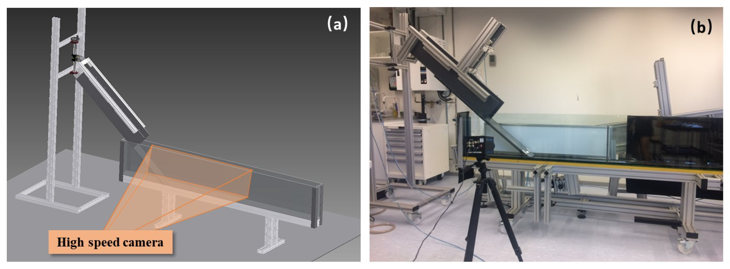
A laboratory experimental system was constructed to investigate landslide-generated waves. Similarity principles were applied to ensure dynamic correspondence between model and prototype. Geometric similarity was set at 1:100. Kinematic similarity was enforced by selecting slide mass and release height to reproduce prototype-consistent entry velocities. Dynamic similarity preserved the Froude number F r for inertia–gravity effects, and introduced the Bingham number B i to capture yield-stress and viscous resistance characteristic of slides. See Section 3.1 for the details of F r and B i . Under these constraints, the laboratory model reproduced the essential physics of landslide-generated waves. The slope was made of PVC (length 1.5 m, width 0.20 m) with adjustable inclination 30°–50°; black sandpaper was bonded to prescribe surface friction. A pneumatically actuated vertical gate at the slope crest restrained the slide until release; the gate opened at 2.5 m/s, after which the slide accelerated downslope and entered water. At the toe, a transparent glass flume (length 2.5 m, depth 0.4 m, width 0.12 m) received the sliding mass; a backlight behind the flume enhanced image contrast. The facilities are summarized in Figure 2. A high-speed camera operating at 400 fps recorded slide motion, water entry, and wave generation. Images were processed in MATLAB 2019 via binary segmentation to extract the pre-entry slide thickness and free-surface profiles. Test conditions were controlled by varying the initial slide mass (from 1000 g to 4000 g) and the gate-to-water distance (from 0.45 m to 0.85 m), while the still-water depth was fixed at 0.2 m and the slope angle was at θ = 45 . More details concern the experimental facilities refer to our previous studies [19,37,52].

2.2. Slide Material

Carbopol was adopted as a soft-soil landslide material to ensure reproducible rheology. Its viscoplastic behavior follows the Herschel–Bulkley relation:
τ = τ c + μ γ ˙ n ,
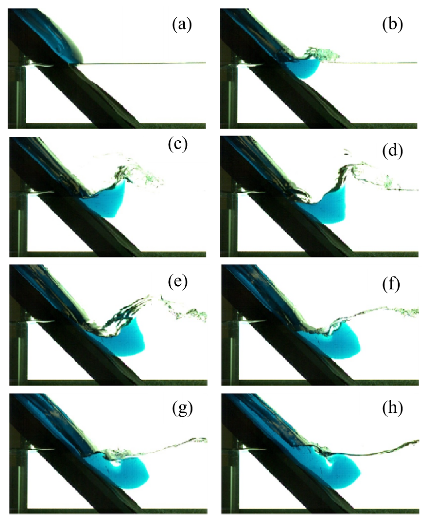
where τ is shear stress, τ c yield stress, μ consistency, γ ˙ shear rate, and n flow index. High-speed observations are shown in Figure 3, documenting a typical sequence from release to attenuation at t = 0 , 100, 150, 200, 250, 300, 350, and 400 ms. The frames reveal downslope acceleration and deformation, water-entry disturbance, crest formation and propagation.

3. Dimensionless Analysis and Variables

3.1. Dimensionless Analysis

In empirical prediction of landslide-generated waves, explanatory variables are selected from key landslide motion parameters, whereas wave characteristics such as wave height and amplitude are treated as dependent variables. After nondimensional transformation, multiplicative power-law forms are fitted to the experimental dataset. A standard expression is as follows:
Ψ n = C i = 1 N X i α i ,
where Ψ n denotes the nth wave characteristics (e.g., wave height, celerity, amplitude), C is a proportional constant, { X i } i = 1 N are selected landslide-related variables, and { α i } are the associated exponents. In this study, wave height h and wave amplitude a are adopted as target variables.
Guided by momentum conservation, the most widely adopted predictors include kinematic and mass measures of the slide. Starting from rest, a slide accelerates along the inclined plane; a fraction of the mass enters the reservoir and generates waves, while the remainder stays on the slope. Influencing factors include the downslope sliding distance, the initial (or effective) mass and the rheology of the slide. Modeling the slide as a viscoplastic fluid, the material parameters are compactly represented through a yield-stress measure, leading to the following functional dependence before nondimensionalization:
Ψ n = F v , m e , s , l 0 , m 0 ; τ c , μ , n .
where the slide entry velocity is v, the gravitational acceleration is g, the effective landslide mass that participates in water entry is m e , the slide thickness at entry is s, whereas the initial thickness before motion is s 0 , the initial downslope sliding distance on the slope is l 0 , the initial landslide mass placed upslope is m 0 , the still-water depth is h 0 , the flume width is B, the water density is ρ w , and the bulk density of the slide material is ρ s .
All variables in Equation (3) are nondimensionalized using characteristic references so that cross-scale comparison is possible and the governing physics can be expressed via a compact set of nondimensional groups. Wave velocity is scaled as a Froude number: F r = v g h 0 ; the effective mass is scaled as relative effective mass: M = m e ρ w B h 0 2 ; thickness is scaled as relative thickness: S = s h 0 ; sliding distance is scaled as relative sliding distance: L = l 0 h 0 ; initial slide mass is scaled as relative initial mass: M i = m 0 ρ w B h 0 2 ; rheological characteristic can be scaled as Bingham number: B i = τ c ρ s s 0 sin θ . The output variables are scaled as relative wave-height and amplitude: H = h h 0 , A = a h 0 .
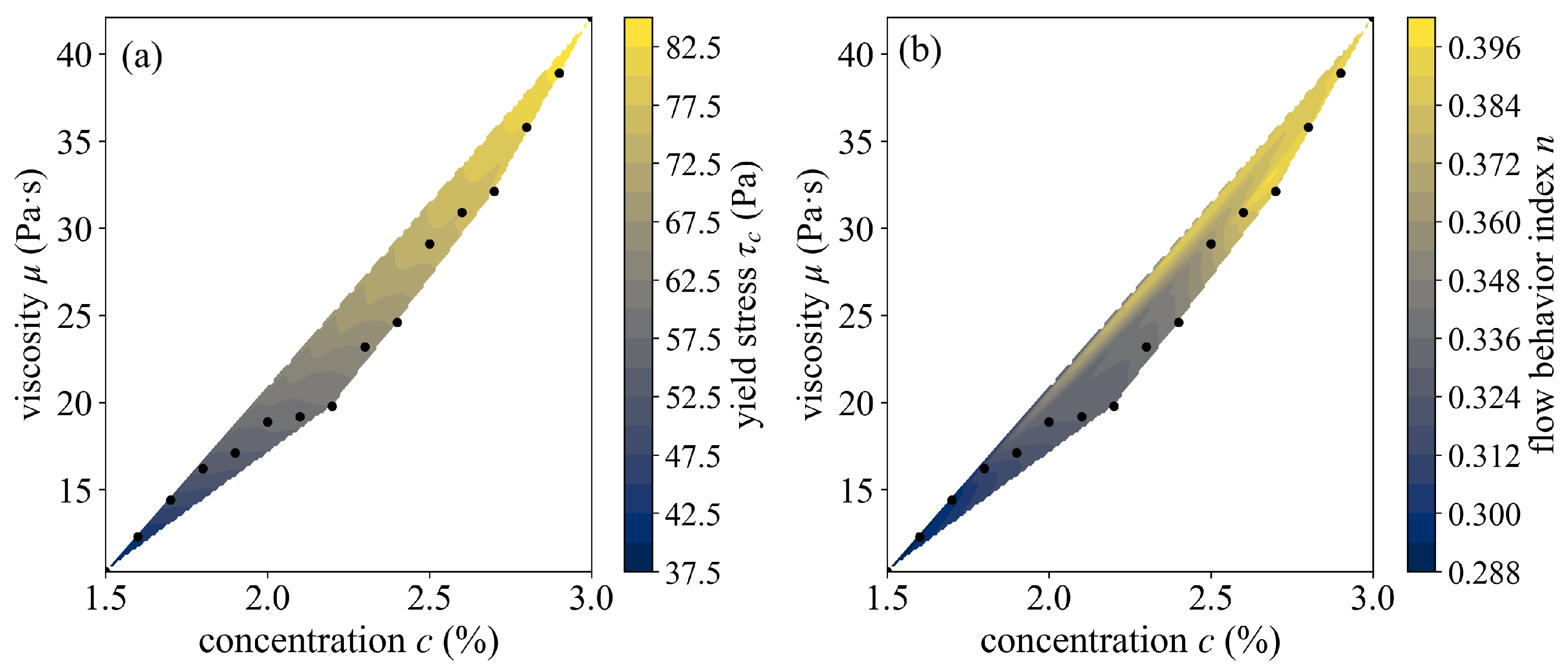
Figure 4 shows that yield stress τ c , consistency μ , and flow index n increase monotonically with concentration of slide material c and are strongly intercorrelated, the Herschel–Bulkley law in Equation (1) mechanistically explains these trends: as c rises, both the yield term and the viscous term grow, so the apparent viscosity η app = τ / γ ˙ = τ c / γ ˙ + μ γ ˙ n 1 increases over relevant shear rates while shear-thinning weakens (since n moves closer to 1). Because entry and early propagation typically involve moderate shear rates where the yield contribution is prominent—and because τ c , μ , and n exhibit near-collinearity—we retain only τ c as the rheological predictor to avoid redundancy and variance inflation while preserving physical interpretability. In practice, higher concentration of slide material c elevates τ c , increases the Bingham number B i used in our scaling.
Two scenarios are considered here to balance physics and practice:
Scenario I uses the slide state at the instant of water entry; the independent variables are the entry Froude number F r , the effective mass ratio M, and the relative thickness S, so the dependence of the targets relative wave amplitude A and relative wave height H can be written as follows:
( A , H ) = F F r , M , S
Scenario II relies on the initial configuration prior to motion; the predictors are the Bingham number B i (rheology), the relative sliding distance L, and the relative initial mass M I , leading to the following:
( A , H ) = F B i , L , M i
These two settings enable prediction either from entry measurements or from initial-state information, broadening the applicability of empirical models.

3.2. Data Distribution

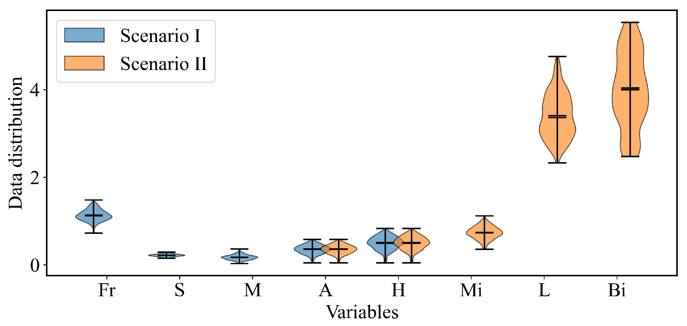
Figure 5 illustrates the distributions of both predictor and target variables for Scenario I and Scenario II. For each variable, two side-by-side violins are shown: the blue violin corresponds to Scenario I and the orange violin to Scenario II. In both Scenario I and Scenario II, the target variables H and A share exactly the same distributions because they are derived from the identical set of 270 experiments; only the explanatory variables differ between these two scenarios. Any comparison across scenarios should not expect differences in H and A distributions, but rather focus on how alternative predictor sets relate to the same outcomes.
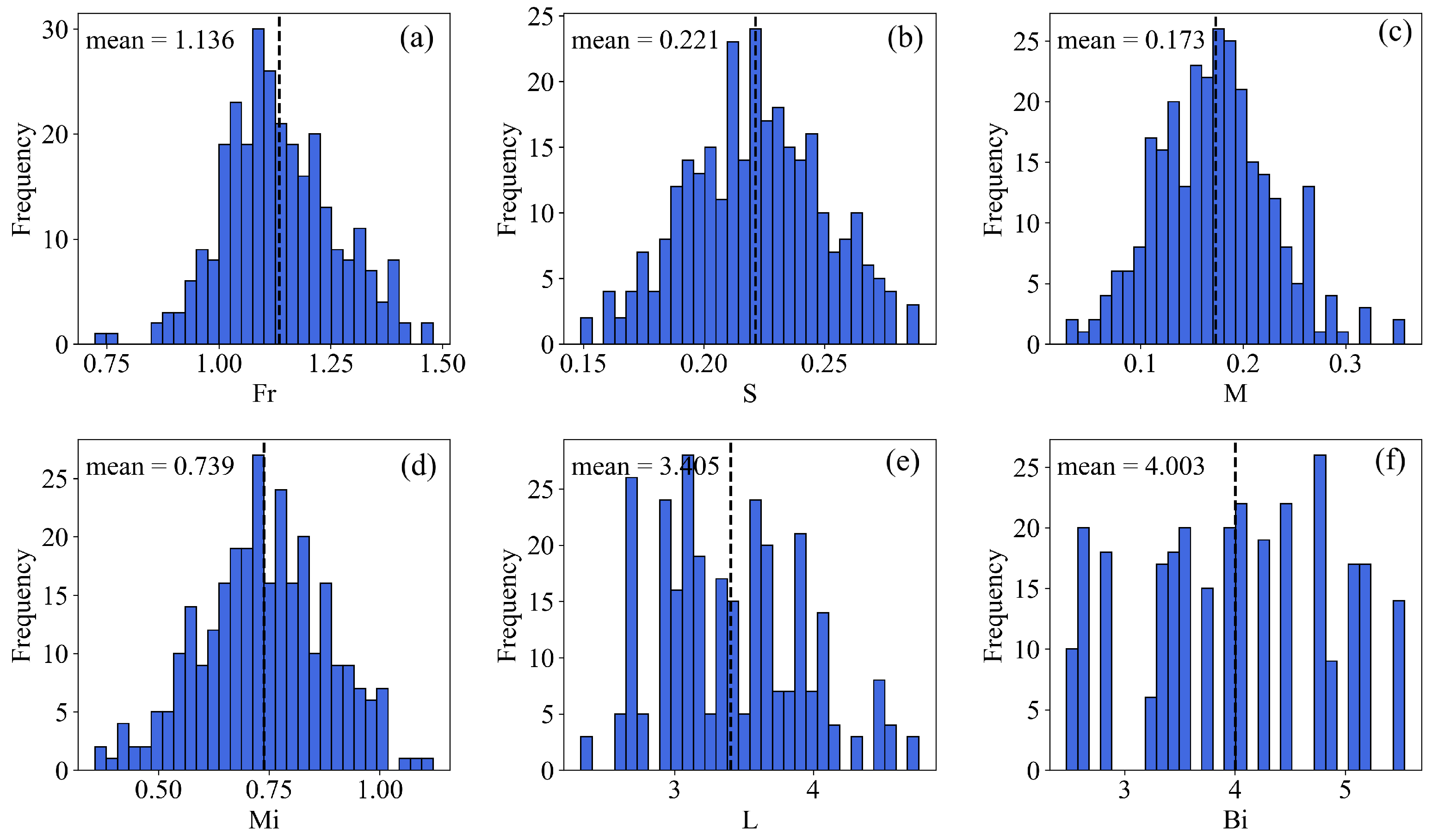
Figure 6 presents the distributions of six predictor variables via 30 equal-width bins. The dashed lines mark sample means. The means of F r , S, M, M i , L, and B i are 1.136, 0.221, 0.173, 0.739, 3.405, and 4.003, respectively. Overall, the predictors are mostly unimodal and approximately symmetric; L shows the tightest spread and highest concentration, whereas B i is the most dispersed with a slight right skew. The remaining variables are fairly balanced around their means, and no pronounced extreme outliers are evident. Although the predictors differ in physical meaning, their coverage and variability are representative for model fitting.
Table 1 indicates that the overall correlations among the predictors are low, which is validated for subsequent modeling: weak inter-predictor correlations yield more stable parameter estimates and improve interpretability. A notable exception is the moderate association between S and M, which is not a statistical artifact but follows from the experimental design and physical constraints. With the material density held constant in our experiments, the mass M scales with the slide volume. Under geometric similarity in a small-scale flume, wave generation is governed by the very short initial entry stage (typically < 0.5 s ), during which the slide geometry exerts primary control on the influx of volume and momentum and hence on the free-surface response. Consequently, increasing M entails a larger total slide volume and larger characteristic dimensions, including S, which naturally produces the observed positive SM correlation in Scenario I. This geometry–mass covariation can not be eliminated under density-controlled and scale-fixed conditions.

4. Modeling Methods

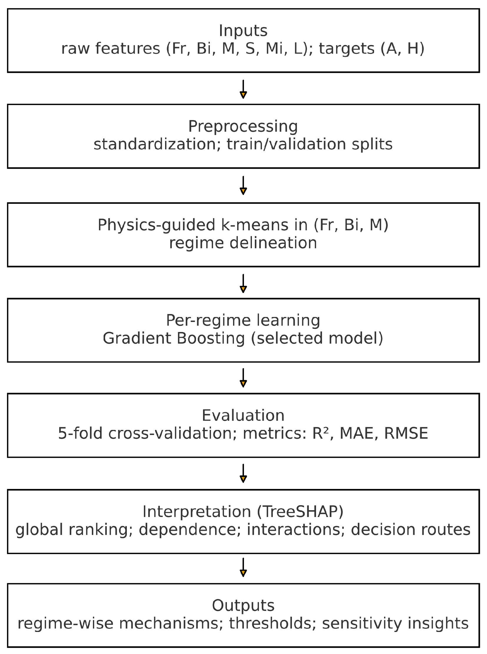
The workflow follows four steps. First, we standardize the inputs and delineate regimes using k-means in ( F r , B i , M ) so that points with similar driving mechanisms are grouped. Second, within each regime we train six predictors to map controls to wave metrics (A and H), and selected the best performing one. Third, we explain the fitted models using SHAP, which attributes each prediction to the contributing parameters in a locally additive and globally aggregable way. Fourth, we synthesize global rankings, marginal effects, and interactions to form regime-wise mechanism statements that are consistent with residual diagnostics. Figure 7 illustrates the overall data-to-model flowchart of the modeling procedure.

4.1. Pre-Clustering via k-Means on ( F r , B i , M )

Before training the prediction model, we separate the dataset into several groups using k-means based on three physical criteria extracted from the two scenarios: the Froude number F r (entry velocity scale), the Bingham number B i (material rheology), and the effective mass ratio M (slide intensity), which jointly capture the dominant kinematic, constitutive, and geometric controls on wave generation [53]. Figure 8 illustrates the schematic of data clustering [54,55]. Given that our emphasis is on SHAP-based interpretation and considering wave characteristics via cluster-defined regimes, we deliberately adopt the mature, widely used, and simple-yet-effective k-means algorithm to keep the clustering step parsimonious.
Let the i-th sample be represented by the following:
z i = F r i , B i i , M i R 3 .
To balance disparate scales and skewness, we standardize the coordinates as follows:
z ˜ i = F r i μ F r σ F r , ψ ( B i i ) , M i μ M σ M ,
Given { x i } i = 1 n in the weighted feature space, k-means seeks cluster centroids { μ c } c = 1 k and assignments { r i c } minimizing the within-cluster sum of squares:
min { r i c } , { μ c } c = 1 k i = 1 n r i c x i μ c 2 2 , r i c { 0 , 1 } , c = 1 k r i c = 1 .
The Lloyd iterations alternate between assignment and update initialized with k-means seeding to improve convergence. The final inertia is as follows:
Inertia = c = 1 k i : r i c = 1 x i μ c 2 2 ,
and k is selected via the elbow and silhouette criterion. Writing centroids back in the physical coordinates helps interpret cluster regimes:
F r ^ c = μ F r + σ F r μ c , F r w F r , B i ^ c = ψ 1 μ c , B i w B i , M ^ c = μ M + σ M μ c , M w M ,
where μ c , ( · ) are centroid components in x-space.

4.2. Gradient Boosting-Based SHAP Analysis for the Two Scenarios

In this study, we benchmarked six machine learning algorithms including gradient boosting, k-nearest neighbors (KNN), XGBoost, linear regression, random forest, and Support Vector Regression (SVR) across two scenarios and two targets using 5-fold cross-validation and multiple evaluation metrics ( R 2 , MAE, RMSE). The comparison indicates that gradient boosting achieves the best overall performance for the present prediction task. See Section 5.2 for details. Thus, we adopt gradient boosting as the focal model and, in what follows, outline its basic principles and how it is coupled with SHAP for interpretable analysis.
Let κ ( i ) { 1 , , k } be the cluster label in Equation (8). We train cluster-specific regressors as follows:
A ^ ( x | κ = c ) , H ^ ( x | κ = c ) for c = 1 , , k ,
We consider two predictor sets as explicated by Equations (4) and (5) and fit them separately:
A ^ = F A ( x ) , H ^ = F H ( x ) , x ( I ) = ( F r , M , S ) , x ( II ) = ( B i , L , M I ) .
Gradient boosting represents the predictor as an additive ensemble of regression trees,
F ( x ) = t = 1 T ν f t ( x ) , f t H = { CART trees } , ν ( 0 , 1 ]
where ν is the learning rate. Given training pairs { ( x i , y i ) } i = 1 n ( y i { A i , H i } ), each boosting step fits a base tree f T to the current pseudo–residuals:
r i ( T ) = y ^ y i , y ^ i ( T 1 ) , ( for squared loss , r i ( T ) = y i y ^ i ( T 1 ) ) ,
optionally followed by a line search to choose the optimal step size:
ρ T = arg min ρ i = 1 n y i , y ^ i ( T 1 ) + ρ f T ( x i ) ,
and the prediction is updated as follows:
y ^ i ( T ) = y ^ i ( T 1 ) + ν ρ T f T ( x i ) .
For our two scenarios (two targets per scenario), the fitted models read as follows:
A ^ ( I ) ( F r , M , S ) = t = 1 T A ν A f t ( I ) , A ( F r , M , S ) , H ^ ( I ) ( F r , M , S ) = t = 1 T H ν H f t ( I ) , H ( F r , M , S ) ,
A ^ ( II ) ( B i , L , M I ) = t = 1 T A ν A f t ( II ) , A ( B i , L , M I ) , H ^ ( II ) ( B i , L , M I ) = t = 1 T H ν H f t ( II ) , H ( B i , L , M I ) .
For a fitted ensemble F and an instance x , SHAP provides an additive decomposition into a baseline and feature contributions:
F ( x ) = ϕ 0 + j = 1 p ϕ j ( x ) , ϕ 0 = E X F ( X ) , p = 3 variables per scenario .
TreeSHAP computes the Shapley values ϕ j ( x ) exactly for tree ensembles by dynamic programming along decision paths, preserving local accuracy in Equation (18). Specializing to our targets and feature sets:
A ^ ( I ) ( F r , M , S ) = ϕ 0 A , ( I ) + ϕ F r A , ( I ) + ϕ M A , ( I ) + ϕ S A , ( I ) ,
H ^ ( I ) ( F r , M , S ) = ϕ 0 H , ( I ) + ϕ F r H , ( I ) + ϕ M H , ( I ) + ϕ S H , ( I ) ,
A ^ ( II ) ( B i , L , M I ) = ϕ 0 A , ( II ) + ϕ B i A , ( II ) + ϕ L A , ( II ) + ϕ M I A , ( II ) ,
H ^ ( II ) ( B i , L , M I ) = ϕ 0 H , ( II ) + ϕ B i H , ( II ) + ϕ L H , ( II ) + ϕ M I H , ( II ) .
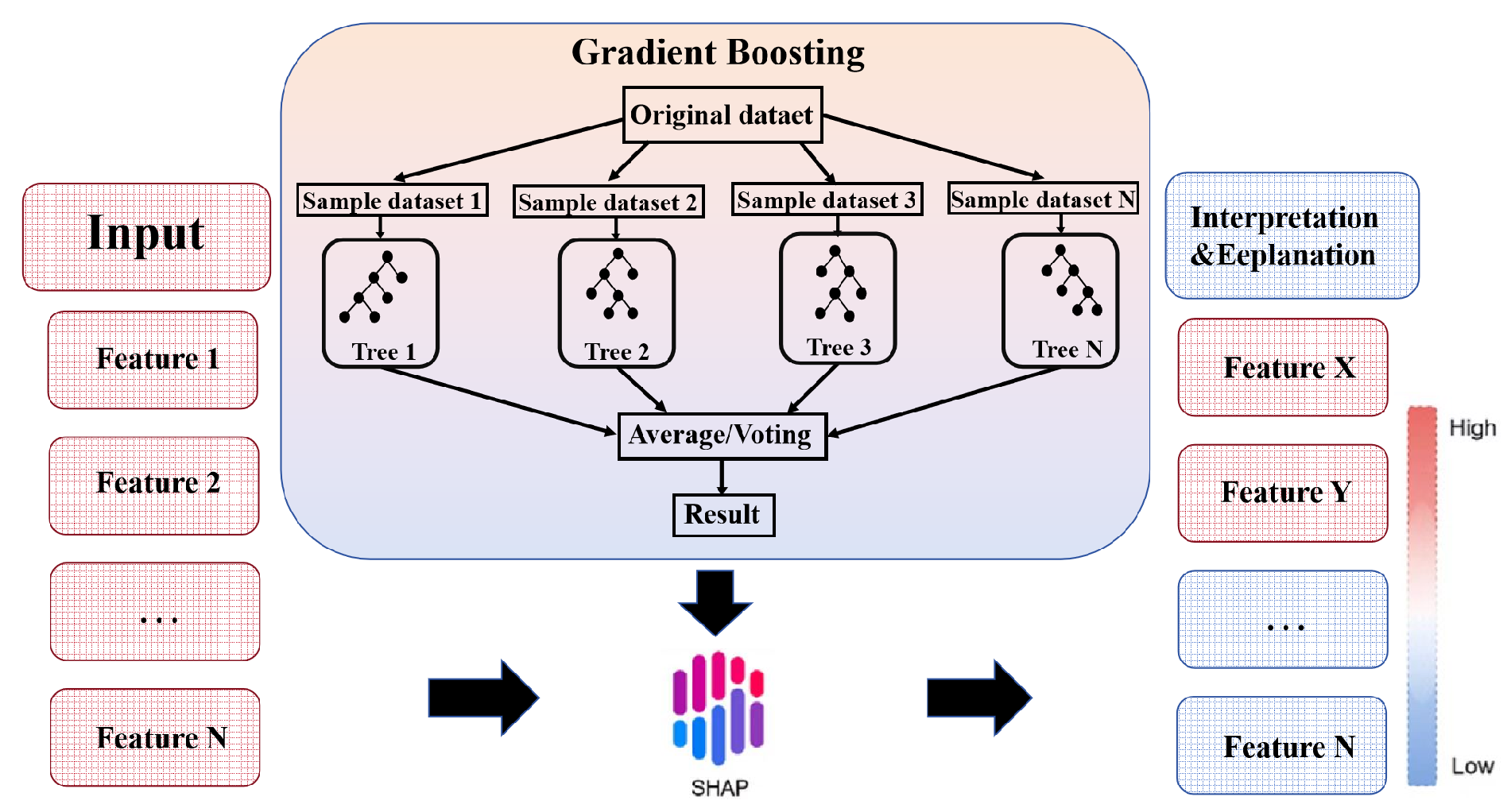
Aggregating { ϕ j ( x i ) } i = 1 n (e.g., by E [ | ϕ j | ] ) yields global importance rankings, while dependence plots visualize each predictor’s local effect on A ^ or H ^ with interaction context encoded the trees. See Figure 9 for the principle of gradient boosting–SHAP frame.

5. Results

5.1. Data Clustering

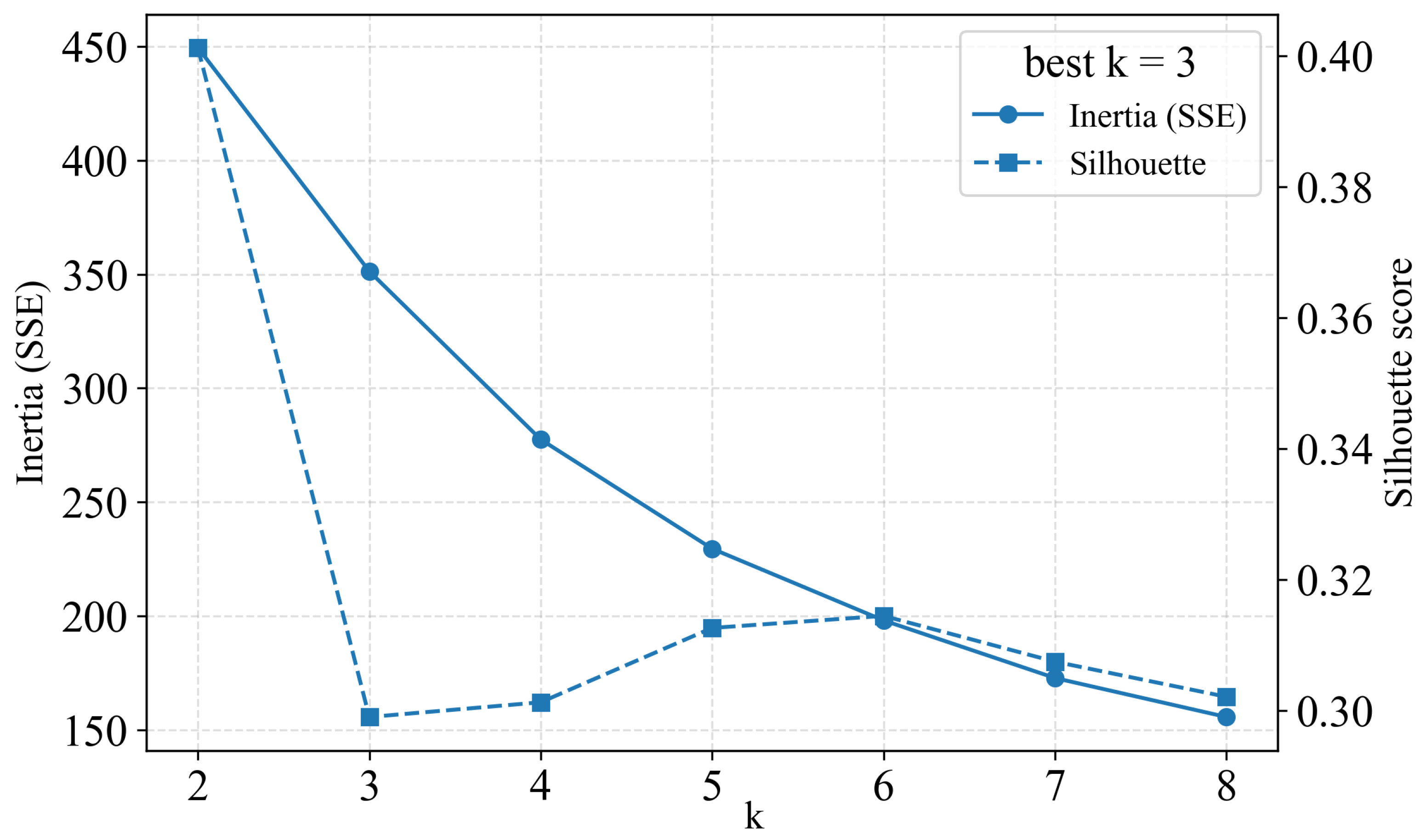
As F r , B i , and M encode entry dynamics, rheological constraint, and slide size respectively, clustering on these nondimensional groups provides a physics-consistent partition of the dataset. Details for the selection of clustering criteria see Section 4.1. Figure 10 presents the selection of cluster number k in ( F r , B i , M ) space. The inertia (SSE) curve shows a pronounced elbow at k = 3 , and the silhouette score attains a comparatively acceptable value at k = 3 . Taken together, these two diagnostics balance intra-cluster compactness (SSE) and inter-cluster separation (sihouette), so we adopt k = 3 for subsequent modeling. We emphasize that these diagnostics are heuristic rather than definitive. The choice k = 3 should therefore be regarded as a pragmatic setting that yields reasonably compact and physically interpretable regimes, while a systematic sensitivity and robustness analysis with respect to k and alternative clustering schemes is left for future work.
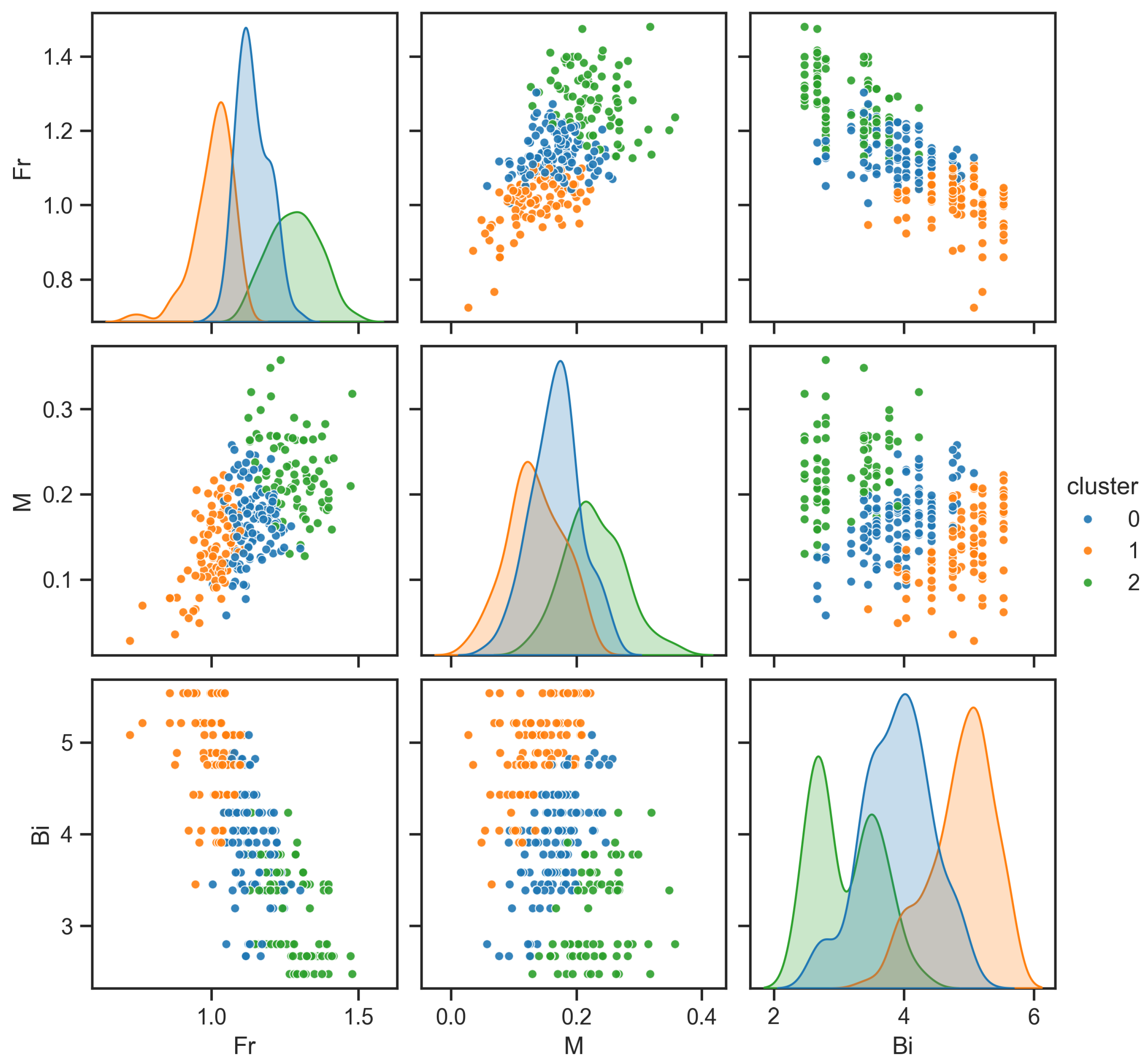
Figure 11 presents the pairwise distributions of the k-means partitions in ( F r , B i , M ) and highlights how the data populate the bivariate planes rather than merely indicating separability. Along ( F r , M ) , the cloud stretches diagonally with modest dispersion, suggesting a coordinated increase in entry speed and effective mass; the diagonal elongation implies anisotropic covariance that is well captured by axis aligned decision boundaries of k-means after standardization. In contrast, ( B i , F r ) and ( B i , M ) display pronounced skew with heavier upper tails in B i at low F r or low M, and compressed spreads where F r or M are large, which is an imprint of yield-limited motion giving way to inertia-dominated entry. Kernel ridges on the diagonals reveal that each cluster admits a distinct internal density profile rather than a simple spherical blob. From a modeling standpoint, this stratification implies reduced heterogeneity within clusters for the predictors.
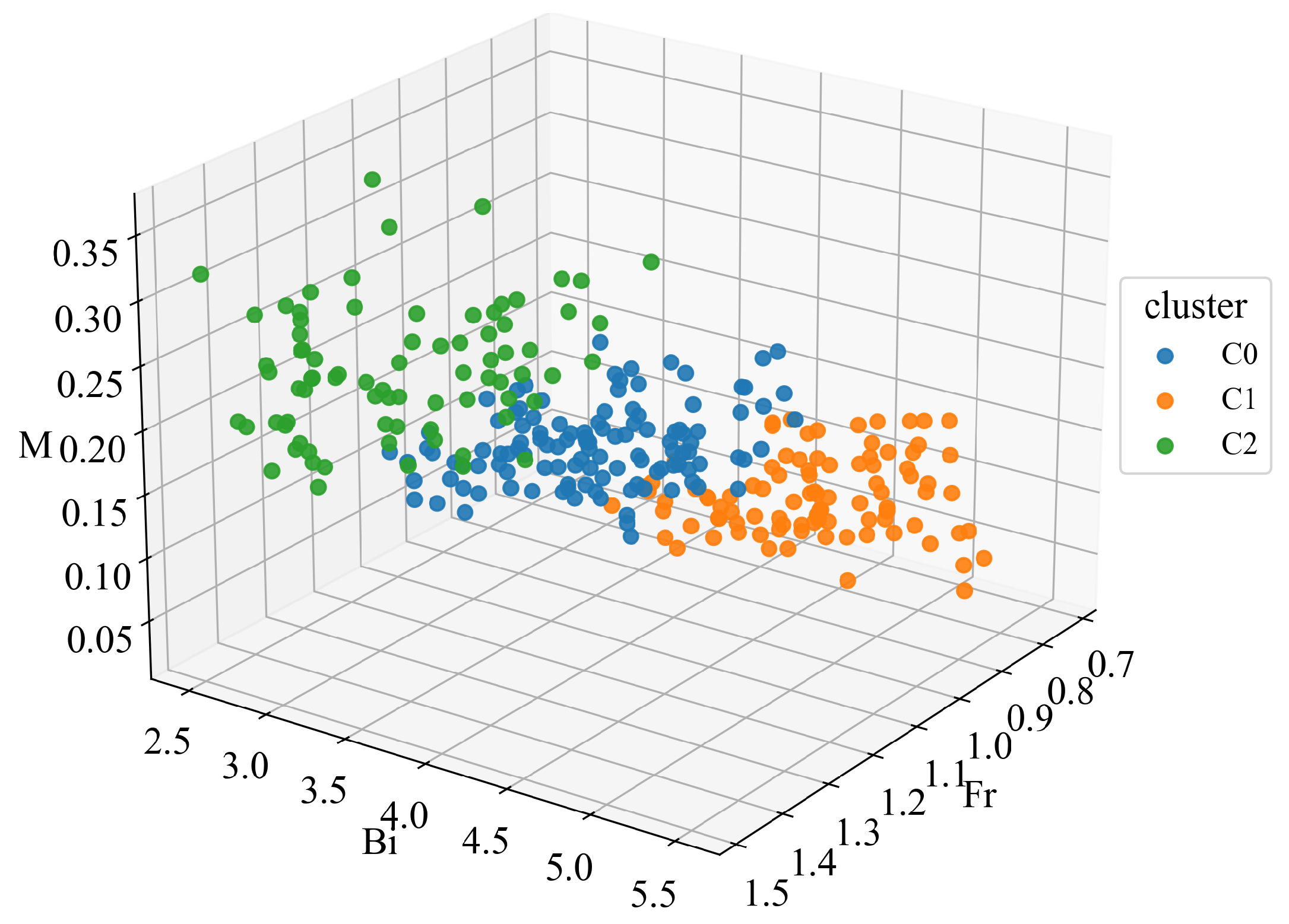
Figure 12 displays the three-dimensional view of the clustering, showing separation primarily along the ( B i , M ) plane with a mild gradient in F r . Points in C1 concentrate at high B i /low M, where yield strength throttles motion and limits energy transfer to the water column; C2 aggregates at low B i /high M, where gravitational–inertial forcing dominates and stronger free surface excitation is expected; C0 bridges the two as geometry and rheology co-control the entry. These physics interpretable groups are then used to condition scenario-specific prediction models— ( F r , M , S ) in Scenario I and ( B i , L , M I ) in Scenario II—for predicting the nondimensional wave amplitude A and height H.

5.2. Prediction Results

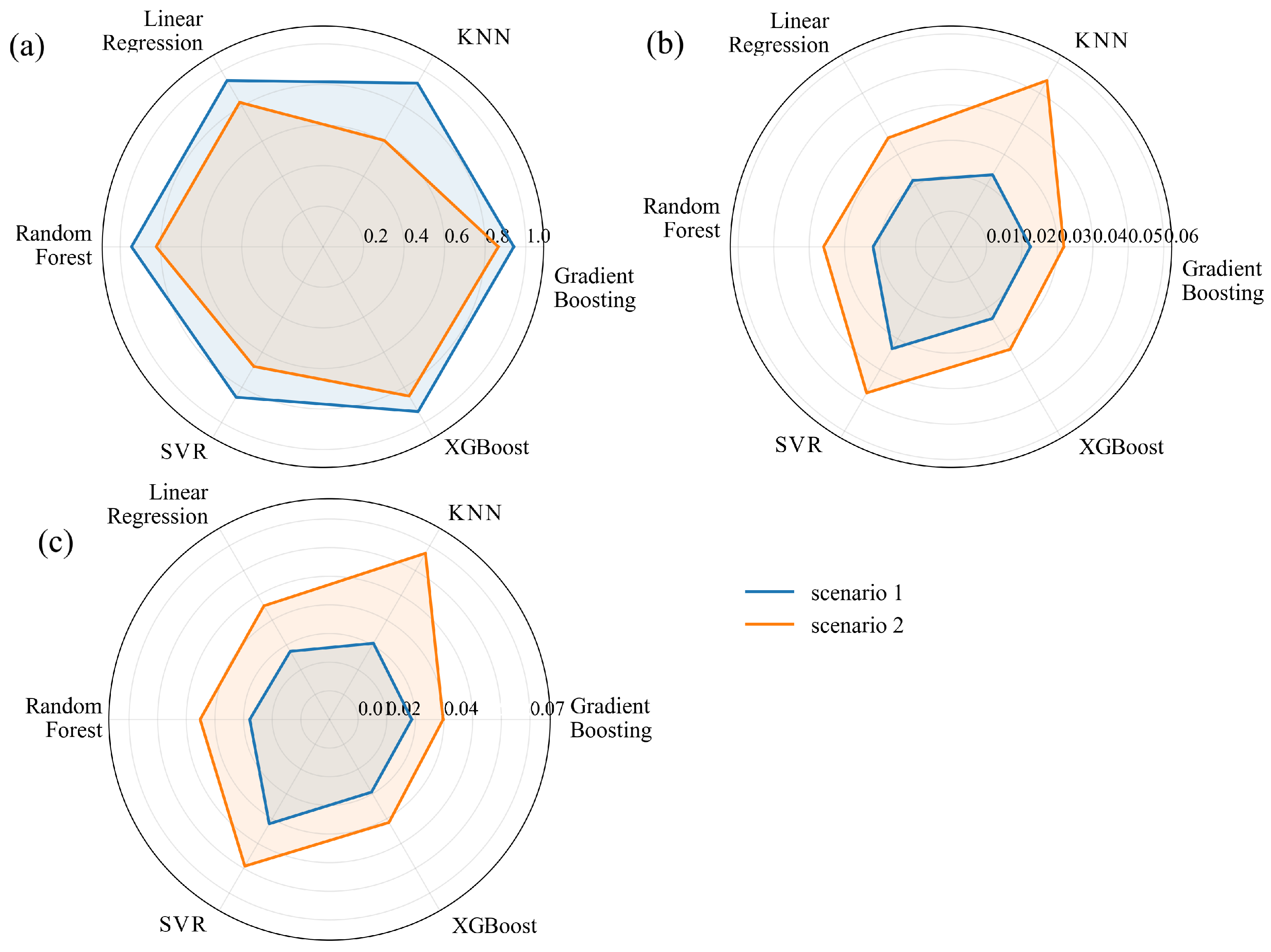
As discussed in Section 3.1, we built prediction models for relative amplitude A and relative height H under two physical settings: scenario I uses the moment of water entry, where feature–target relationships are more direct, and scenario II uses the moment when the landslide comes to rest. We compared six common machine-learning algorithms, including gradient boosting, KNN, XGboost, linear regression, random forest, and SVR, and then evaluated model validity and generalization with 5-fold cross-validation per-cluster, averaging fold-wise R 2 , MAE, and RMSE and monitoring variability. As shown in Figure 13, scenario I achieves higher overall accuracy than scenario II. This is because scenario I starts from water entry with more direct feature–target association, while scenario II starts after the slide stops and involves a more complex physical process that the three variables cannot fully represent, its overall accuracy is generally lower than scenario I. For both the two scenarios, XGboost and gradient boosting perform very similarly, their R 2 in the more complex scenario II still exceeds 0.85, but gradient boosting is slightly better in aggregate metrics and cross-scenario consistency.
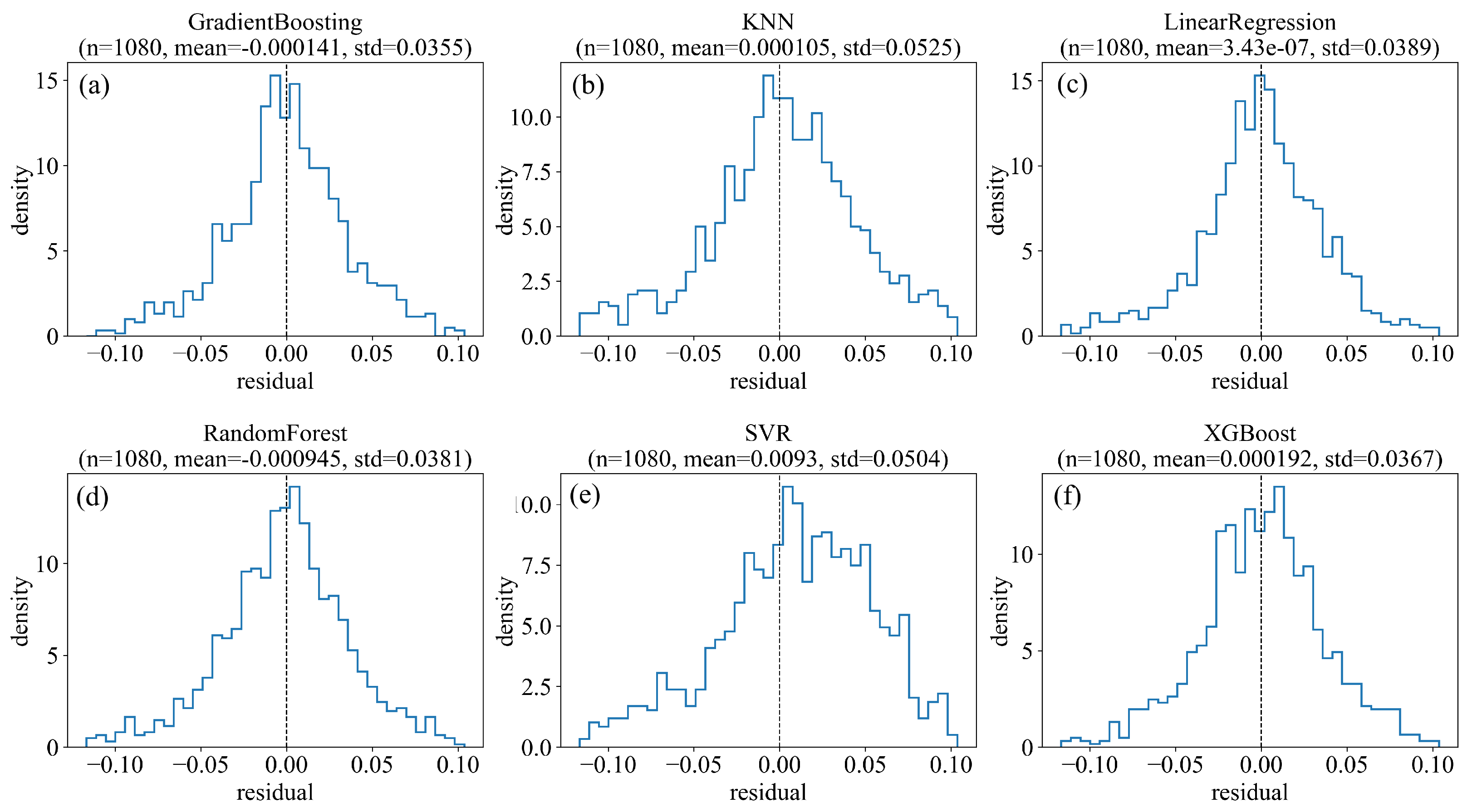
Figure 14 shows the residual distributions of the six models after pooling data from both scenarios (I and II) and both target variables (H and A). Each scenario–target combination contributes 270 samples, yielding 1080 residuals in total. All histograms are centered near zero with means close to 0, indicating negligible bias. Distribution width reflects typical error and tail thickness reflects the risk of large errors. gradient boosting and XGBoost show the narrowest, light-tailed spreads, random forest and linear regression are intermediate, and KNN and SVR display wider, heavier-tailed residuals. Consistent with the radar-plot ranking, we therefore adopt gradient boosting as the baseline for TreeSHAP interpretation.
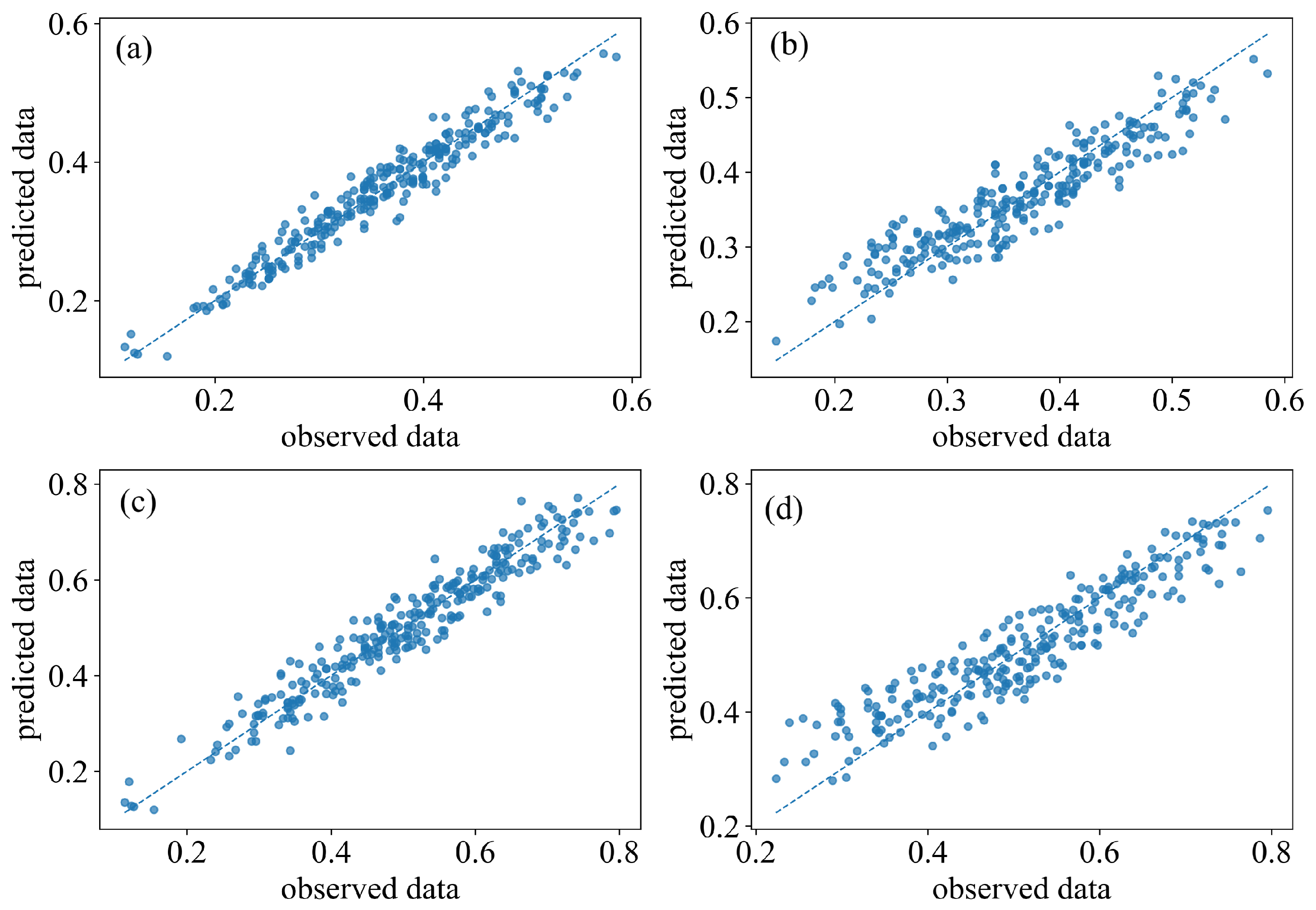
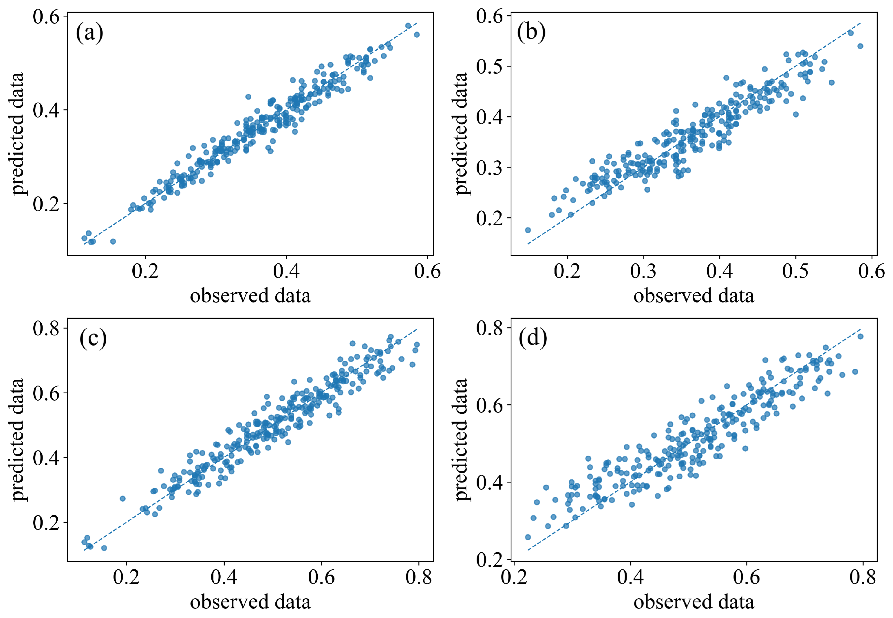
Figure 15 presents the observed–predicted comparisons for the selected best model, gradient boosting: (a) A in scenario I, (b) A in scenario II, (c) H in scenario I, and (d) H in scenario II. In all four panels, the points cluster closely around the 1 : 1 line, indicating overall good agreement. Visually, the clouds for scenario I (a, c) are tighter and adhere more closely to the reference line than those for scenario II (b, d), confirming that scenario I achieves higher overall fidelity, which are consistent with Figure 13 and Figure 14. A few high–value samples show mild deviations, but they do not alter the overall conclusion. The observed–predicted plots for the other models are provided in the Appendix B for side-by-side comparison. In brief, we proceed by coupling the gradient boosting model with SHAP in the following Section 5.3 to enable interpretable analysis of feature contributions.

5.3. Interpretation Analysis Based on SHAP

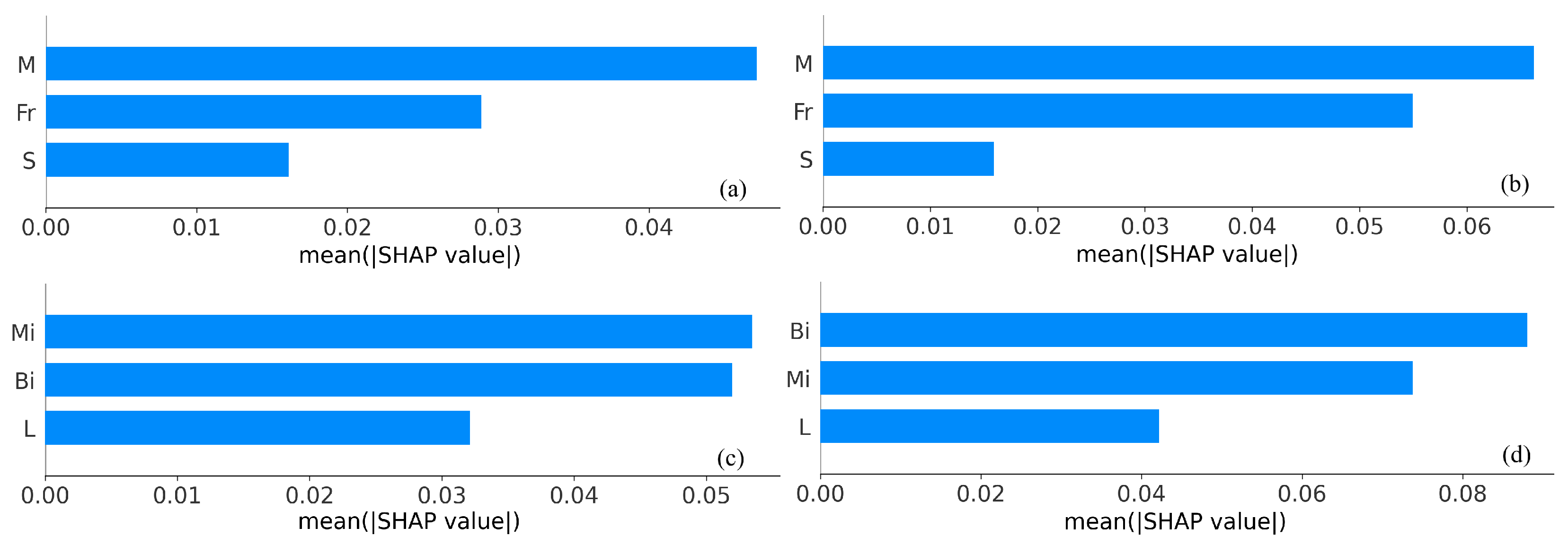
As shown in Figure 16, Scenario I ranks M > F r > S for both A and H. Scenario II shows A co-led by M i and B i with L smaller, while H is led by B i then M i . The prominence of M in Scenario I aligns with a momentum–impulse control: larger effective mass injects a stronger impulse at entry. F r modulates inertial forcing relative to gravity, and S acts mainly as geometric tuning. In Scenario II, M i dictates available momentum and B i preserves slide coherence, jointly strengthening wave making; L contributes less by reflecting path-length–related dissipation.
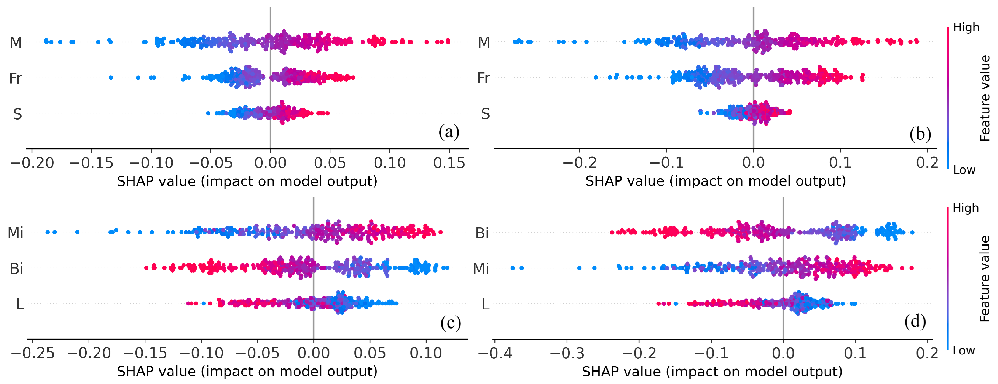
Figure 17 summarizes distributional effects. Wider spreads indicate stronger influence, and the sign of SHAP values indicates tendency. In Scenario I, M and F r show the widest spreads and mostly positive contributions, whereas S is weaker and centered near zero. In Scenario II, M i and B i dominate, typically increasing A and H; L is narrower and often slightly negative, consistent with dissipation over longer travel.
Figure 18 traces decision routes from the base value to each prediction. Early, steep segments identify variance-dominant features. Scenario I routes diverge primarily along M and F r , with S making later, smaller adjustments. Scenario II routes turn first on M i and B i , indicating that initial mass and rheology set how much energy reaches the free surface, while L shifts trajectories later by altering forcing duration. The broader route ranges in Scenario II reflect stronger mass–rheology coupling than purely geometric effects.
Table 2 presents the feature interaction strengths across the two target variables at the two scenarios. In Scenario I, the leading pair ( F r , S ) shows that thickness effects are amplified at higher inertia: as the slide moves faster relative to gravity, small changes in S generate disproportionately larger pressure impulses and longer effective contact, boosting A and H. The ( F r , M ) coupling aligns with impulse scaling: for a given velocity regime, added mass increases momentum, and the gain is realized most strongly when inertia dominates. The ( S , M ) pairing suggests geometric–mass synergy: thicker, heavier slides maintain contact and transmit load more coherently, enhancing wave efficiency beyond additive effects. In Scenario II, the strong ( M i , B i ) interaction points to a mass–rheology control: more material coupled with higher yield strength preserves slide integrity and elevates the effective pressure history at the free surface, producing larger waves. The subsequent pairs, ( M i , L ) and ( L , B i ) , indicate that both added mass and increased rheological stiffness are more impactful when the slide travels farther: a longer path sustains forcing, but whether that extra duration converts to wave growth depends on how coherently stress is transmitted and how much momentum is carried. The systematically larger interaction magnitudes in Scenario II are consistent with a rheology-limited regime.
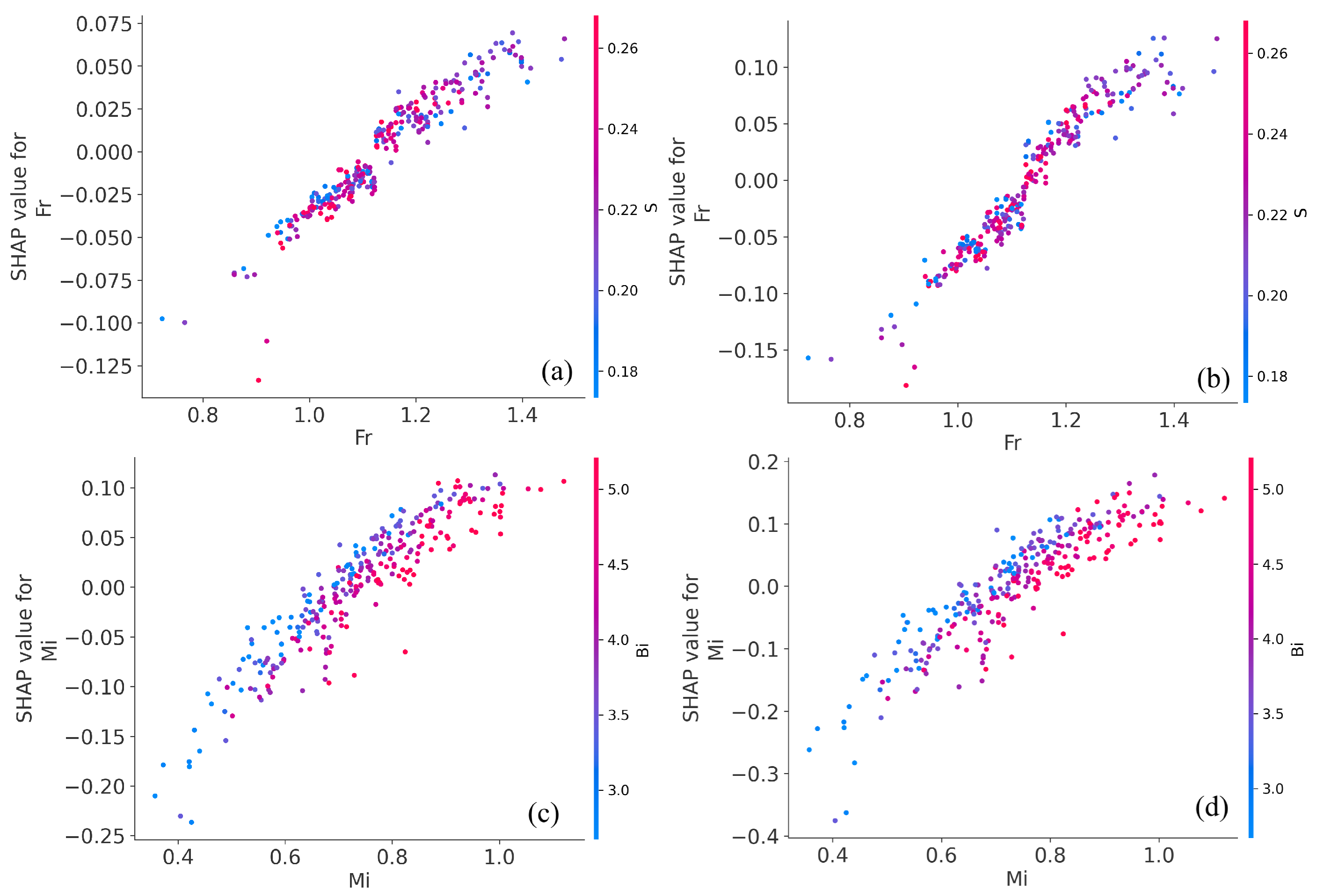
Figure 19 shows the SHAP dependence of the most influential interaction in each setting: ( F r , S ) for Scenario I and ( M i , B i ) for Scenario II. Points plot the SHAP value of the horizontal-axis feature against its raw value; color encodes the interacting feature (warmer = larger). In Scenario I, F r exhibits a clear positive, near-monotonic relation with its SHAP value, and warmer colors (larger S) shift the points upward, indicating synergy: thickness amplifies the inertial contribution of F r to both A and H. In Scenario II, M i likewise shows a strong positive trend, with warmer colors (larger B i ) producing higher SHAP values, consistent with mass–rheology coupling: more initial mass delivered through a stiffer, more coherent slide (higher B i ) enhances wave generation. The steeper slopes and stronger color separation in Scenario II highlight that these joint effects are greater there than in Scenario I.
Figure 20 presents 2D dependence maps for the same top interaction pairs as Figure 19, showing model output over the ( F r , S ) and ( M i , B i ) planes. Brighter regions indicate larger predicted responses. In Scenario I, the maps increase toward the high F r , high S corner, confirming that greater inertia combined with thicker slides yields larger waves, with mild nonlinearity along F r . In Scenario II, the surfaces rise most strongly toward high M i , high B i , evidencing pronounced synergy between available mass and rheological coherence. The sharper gradients and broader bright plateaus in Scenario II are consistent with a regime where rheology–mass coupling, rather than geometry alone, governs how efficiently input momentum is converted into the scaled wave amplitude and height.

6. Discussions

6.1. Key Findings and New Insights from Interpretability

Across scenarios, residuals are centered near zero and model rankings are consistent across cross-validated metrics and error distributions. TreeSHAP reveals regime-dependent controls that extend beyond earlier linear or globally averaged analyses. In Scenario I (entry-state features F r , M , S ), mass is the leading driver and the inertia–geometry interaction ( F r × S ) amplifies energy injection at higher inertia. In Scenario II (pre-motion features B i , L , M i ), initial mass and rheology jointly dominate, with the M i × B i interaction maintaining slide coherence and stress transmission. Partitioned, cluster-wise modeling reduces cross-mechanism averaging and links global rankings, marginal effects, and local decision routes into a coherent mechanism chain.

6.2. Practical Significance and Geological Translation

The interpretability results translate into concrete decisions for landslide-generated wave risk. Pre-motion variables ( B i , M i , L ) support rapid triage of slopes before motion; dependence curves provide thresholds that indicate when combinations of features become hazardous; and interaction maps point to locations where monitoring will be most informative. These insights guide the prioritization of measurements, the placement of sensors, and the exploration of mitigation options through sensitivity-based “what-if” analysis. Because gradient boosting exhibits narrower, lighter-tailed residuals, it is adopted as the TreeSHAP baseline to limit the risk of large errors in decision support.
Model inputs are operationalized as field observables as follows: M approximates the mobilized volume inferred from scar geometry and bulk density; F r serves as an inertia proxy estimated from drop height and runout metrics; S represents local bathymetry and basin confinement; and ( B i , M i , L ) correspond to density contrast and water depth B i , material and rheological indicators M i , and effective path roughness L. Conditional on these mappings, narrow and steeply confined basins such as fjord and reservoir embayments with elevated F r and large S are expected to amplify wave energy, whereas wide, gently sloping shelves are expected to enhance dissipation. Dependence curves are used as screening thresholds, and interaction maps inform sensor placement near regime boundaries where extrapolation risk increases. Principal limitations include unmodeled pore-pressure transients, mass fragmentation or entrainment, site-specific roughness, and the distinction between model attribution and causality. To mitigate these issues, we adopt conservative alert thresholds guided by residual spread, impose simple physics-based constraints within clusters, and prioritize rapid field proxies for M i and B i .

6.3. Physics–Data Trade-Offs and Generalization Beyond Laboratory Settings

The two-scenario design makes explicit the balance between physical fidelity and operational applicability. Scenario I isolates entry-state dynamics for clearer mechanism identification but requires estimation of entry-state variables from pre-event data. Scenario II relies only on pre-motion inputs, trading some predictive accuracy for usability before a slide occurs. Physics-informed structure within clusters, such as monotonicity, dimensional consistency, and convexity, can reduce this gap while retaining flexibility in data fitting. For deployment under domain shift, clustering delineates regime boundaries where extrapolation risk increases; conservative alert thresholds, uncertainty flags based on residual spread and range checks, and mixture-of-experts models with physical constraints are recommended to improve transfer across regimes. At present, this physics–data balance is assessed only on 270 controlled laboratory runs; extending the workflow to independent field datasets and additional experimental facilities remains a key step before operational deployment.

6.4. Field Validation and Limitations

Field validation can proceed through hindcasting documented events with site-specific bathymetry and topography, prospective comparisons at instrumented slopes using GNSS/InSAR and water-level records, and leave-location-out evaluations to quantify cross-site transferability. Current limitations include sparse coverage in parts of the feature space that can distort partial effects, attribution under correlation where SHAP explains the model rather than causality, and potential instability of k-means boundaries near regime transitions. Future work will incorporate bootstrap or Bayesian uncertainty quantification, additional physics-guided constraints within clusters, and the field programs outlined above.

7. Conclusions

This work assembles a concise, interpretable, and scenario-aware workflow for landslide-generated waves by combining physics-guided k-means clustering, per-cluster gradient boosting, and SHAP-based attribution. Clustering in ( F r , B i , M ) yields regimes that are both physically meaningful and operationally available prior to prediction, enabling models to learn regime-specific controls and supporting transparent explanations of amplitude A and height H. Across six benchmarked learners under unified 5-fold cross-validation (R2, MAE, RMSE), gradient boosting is the top performer with strong cross-scenario robustness, and XGBoost is a close second. Scenario I (water-entry state) attains higher accuracy than Scenario II (pre-motion), consistent with stronger feature–target coupling at entry; nevertheless, Scenario II maintains high skill (R2 > 0.85 in our data).
TreeSHAP provides a mechanism-centered synthesis rather than a summary of plots. In Scenario I, inertia and mass dominate with a clear inertia–geometry synergy F r × S that amplifies energy injection; in Scenario II, initial mass and rheology co-dominate, with M i × B i preserving slide coherence and stress transmission. The regime-wise design avoids cross-mechanism averaging, linking global rankings, marginal effects, and local decision routes into a consistent account of when and why waves intensify. These insights have practical impact for hazard forecasting and design. Pre-motion variables ( B i , M i , L ) support rapid screening and the setting of SHAP-derived alert thresholds; interaction hotspots indicate where to prioritize measurements and sensor placement.
Limitations include potential sampling sparsity, attribution shifts under correlated predictors, heuristic cluster selection, and the laboratory scale of the dataset. Future work will (i) perform site-specific hindcasting and leave-location-out tests for external validation and (ii) embed physics-informed constraints within clusters to reduce trade-offs between fidelity and actionability.

Author Contributions

Conceptualization, Z.M.; methodology, X.X. and P.Q.; validation, X.X., Z.L. and J.W.; formal analysis, X.X., Y.Z. and S.Z.; data curation, Z.M.; writing—original draft preparation, X.X.; writing—review and editing, P.Q. and Z.M.; supervision, P.Q. and Z.M.; funding acquisition, P.Q. and Z.M. All authors have read and agreed to the published version of the manuscript.

Funding

This research was funded by Zhejiang Provincial Natural Science Foundation of China (Grant No. LZJWY24E090005, LTGG24E090001), Huzhou Science and Technology Plan Project (Grant No. 2024G263), the Student Innovation and Entrepreneurship Training Program at Zhejiang University of Water Resources and Electric Power (2025), Program of “Xinmiao” (Potential) Talents in Zhejiang Province (Grant No. 2025R422A001), Central Guidance Funds for Science and Technology Local Development Projects (Grant No. 2025ZY01091).

Data Availability Statement

Data available upon request.

Conflicts of Interest

The authors declare no conflicts of interest.

Appendix A. End-to-End Pipeline of the Modeling Procedure

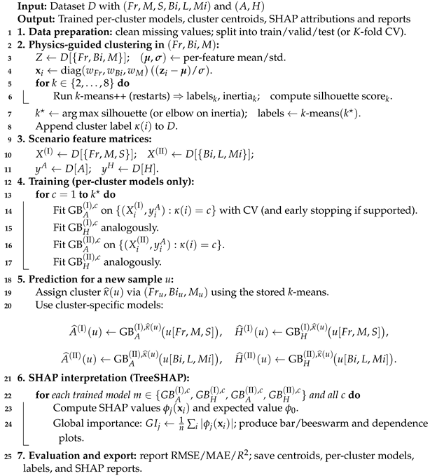
We assume a dataset D with predictors ( F r , M , S , B i , L , M i ) and targets ( A , H ) . Clustering is performed in the physics-guided subspace z i = ( F r i , B i i , M i i ) R 3 . Scenario-specific design matrices are train separate models for A and H: x i ( I ) = ( F r i , M i , S i ) , x i ( II ) = ( B i i , L i , M i i ) . Algorithm A1 presents the end-to-end pseudocode of the whole modeling process: k-means clustering, gradient boosting prediction per-cluster, SHAP interpretation.
Algorithm 1: End-to-end pseudocode: k-means clustering → gradient boosting prediction per-cluster → SHAP interpretation.
Jmse 13 02223 i001

Appendix B. Additional Model Comparisons
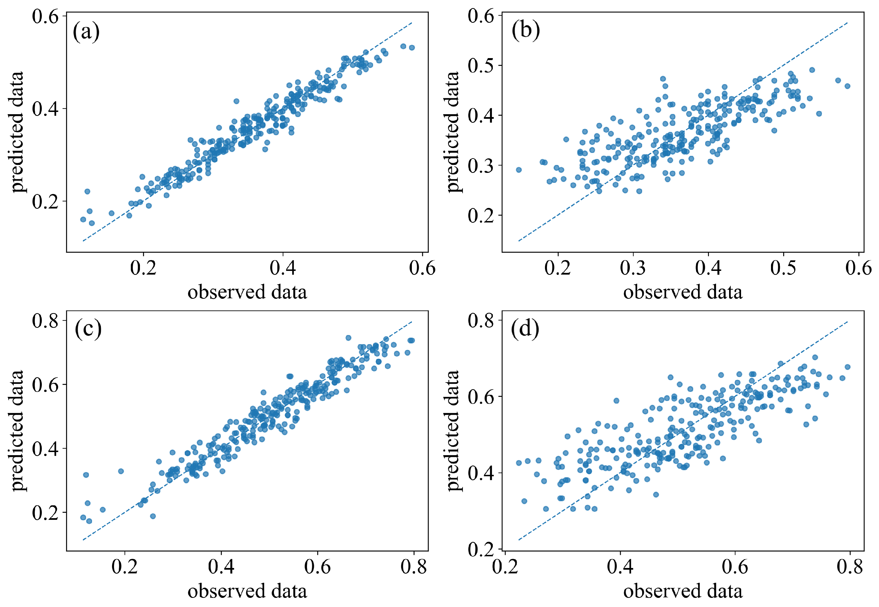
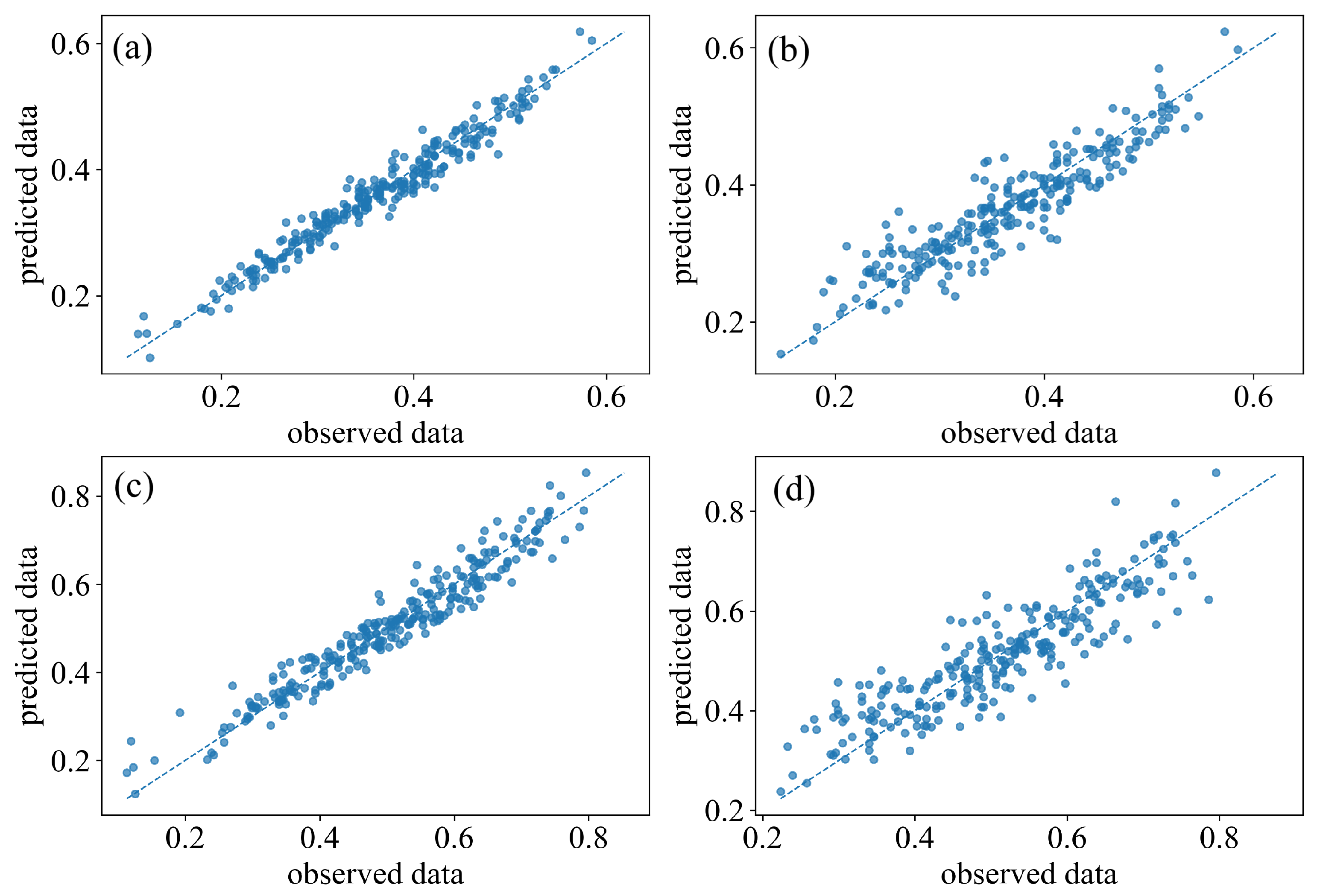
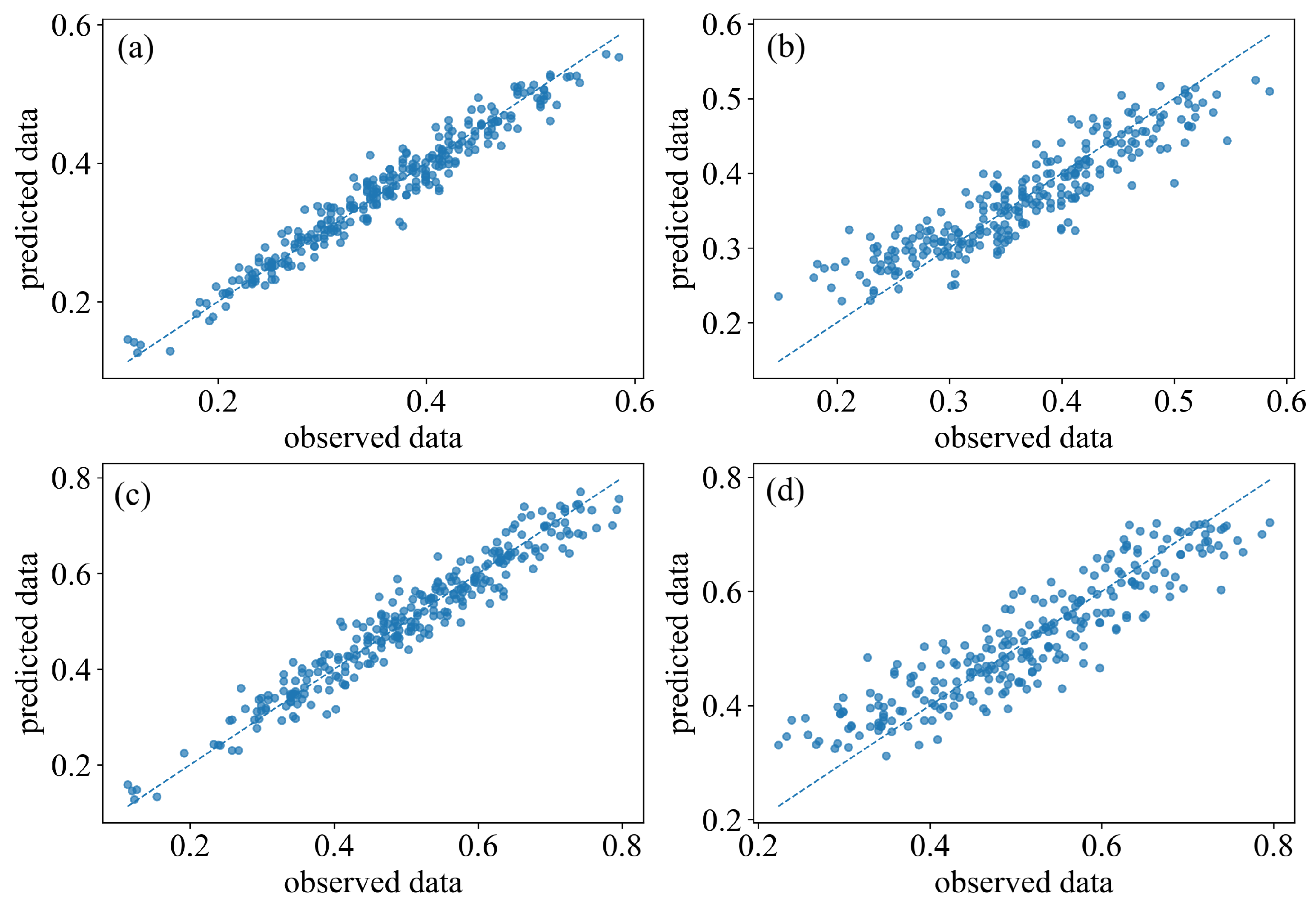
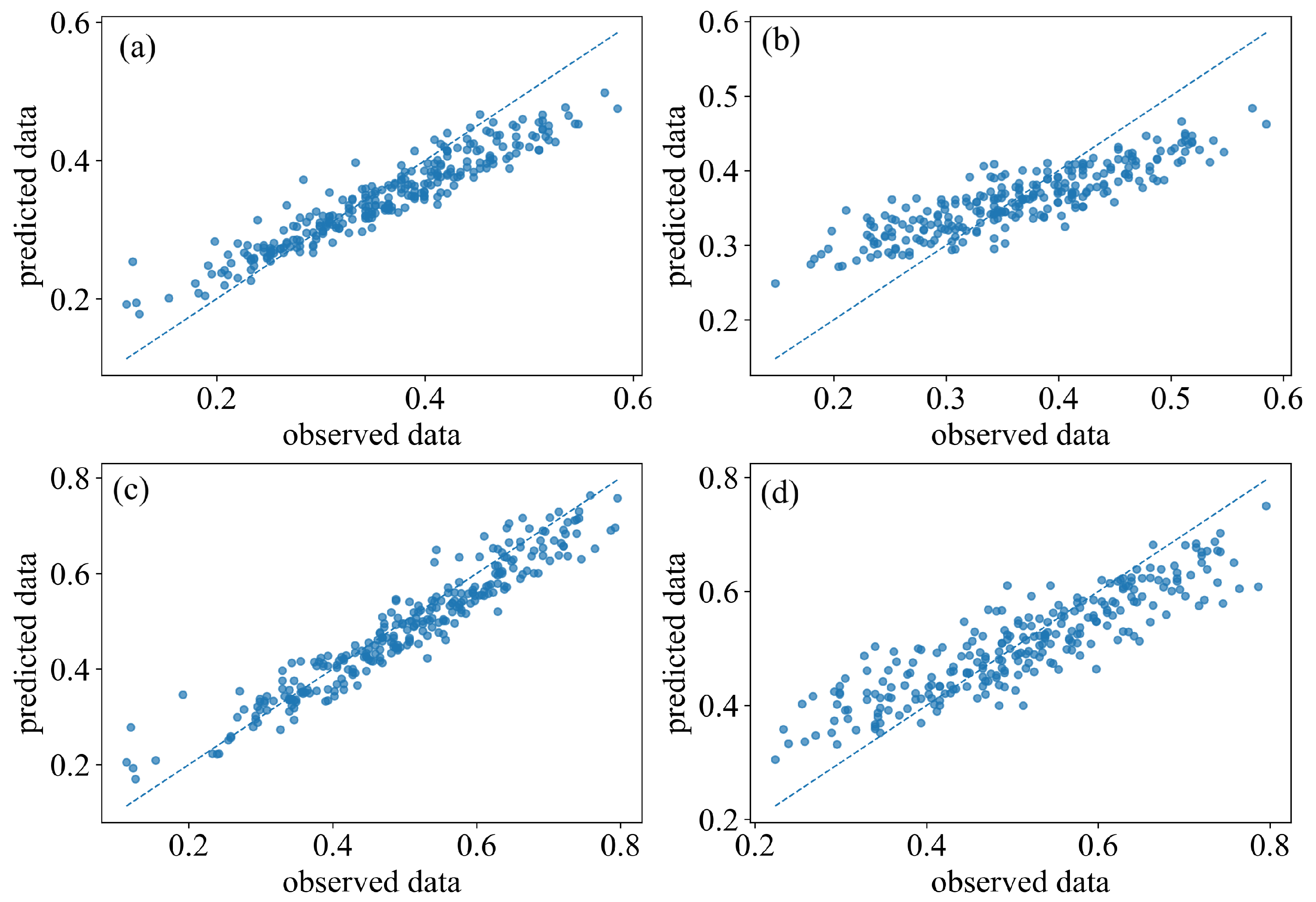
Figure A1, Figure A2, Figure A3, Figure A4 and Figure A5 compile the observed–predicted scatter plots for the remaining models—KNN, XGBoost, linear regression, random forest, and SVR—across both scenarios (I and II) and both target variables (H and A). Axis limits and the 1 : 1 reference line are kept consistent with the main text for direct visual comparison. As anticipated, the patterns mirror the aggregate findings: scenario I generally exhibits tighter clouds and smaller dispersion than scenario II, while model–specific differences in spread and alignment with the 1 : 1 line highlight each method’s stability and bias characteristics. These panels are intended to complement Figure 15, enabling side-by-side assessment of model behavior under the two physical settings.
Figure A1. Comparison of the observed data with predicted data of KNN model: (a) A (scenario I); (b) A (scenario II); (c) H (scenario I); (d) H (scenario II).
Jmse 13 02223 g0a1
Figure A2. Comparison of the observed data with predicted data of linear regression: (a) A (scenario I); (b) A (scenario II); (c) H (scenario I); (d) H (scenario II).
Jmse 13 02223 g0a2
Figure A3. Comparison of the observed data with predicted data of random forest model: (a) A (scenario I); (b) A (scenario II); (c) H (scenario I); (d) H (scenario II).
Jmse 13 02223 g0a3
Figure A4. Comparison of the observed data with predicted data of SVR: (a) A (scenario I); (b) A (scenario II); (c) H (scenario I); (d) H (scenario II).
Jmse 13 02223 g0a4
Figure A5. Comparison of the observed data with predicted data of XGBoost model: (a) A (scenario I); (b) A (scenario II); (c) H (scenario I); (d) H (scenario II).
Jmse 13 02223 g0a5

References

  1. Løvholt, F.; Pedersen, G.; Harbitz, C.B.; Glimsdal, S.; Kim, J. On the characteristics of landslide tsunamis. Philos. Trans. R. Soc. A Math. Phys. Eng. Sci. 2015, 373, 20140376. [Google Scholar] [CrossRef] [PubMed]
  2. Ward, S.N. Landslide tsunami. J. Geophys. Res. Solid Earth 2001, 106, 11201–11215. [Google Scholar] [CrossRef]
  3. Gao, J.; Ma, X.; Chen, H.; Zang, J.; Dong, G. On hydrodynamic characteristics of transient harbor resonance excited by double solitary waves. Ocean. Eng. 2021, 219, 108345. [Google Scholar] [CrossRef]
  4. Heller, V.; Hager, W.H.; Minor, H.E. Scale effects in subaerial landslide generated impulse waves. Exp. Fluids 2008, 44, 691–703. [Google Scholar] [CrossRef]
  5. Heller, V.; Hager, W.H. Impulse product parameter in landslide generated impulse waves. J. Waterw. Port Coast. Ocean. Eng. 2010, 136, 145–155. [Google Scholar] [CrossRef]
  6. Lynett, P.; Liu, P.L.F. A numerical study of submarine–landslide–generated waves and run–up. Proc. R. Soc. London Ser. A Math. Phys. Eng. Sci. 2002, 458, 2885–2910. [Google Scholar] [CrossRef]
  7. Panizzo, A.; De Girolamo, P.; Petaccia, A. Forecasting impulse waves generated by subaerial landslides. J. Geophys. Res. Ocean. 2005, 110, C12025. [Google Scholar] [CrossRef]
  8. Walder, J.S.; Watts, P.; Sorensen, O.E.; Janssen, K. Tsunamis generated by subaerial mass flows. J. Geophys. Res. Solid Earth 2003, 108, 2236. [Google Scholar] [CrossRef]
  9. Heller, V.; Spinneken, J. On the effect of the water body geometry on landslide–tsunamis: Physical insight from laboratory tests and 2D to 3D wave parameter transformation. Coast. Eng. 2015, 104, 113–134. [Google Scholar] [CrossRef]
  10. Fritz, H.M.; Hager, W.H.; Minor, H.E. Near field characteristics of landslide generated impulse waves. J. Waterw. Port Coastal Ocean. Eng. 2004, 130, 287–302. [Google Scholar] [CrossRef]
  11. Evers, F.M.; Hager, W.H. Spatial impulse waves: Wave height decay experiments at laboratory scale. Landslides 2016, 13, 1395–1403. [Google Scholar] [CrossRef]
  12. Mao, P.; Lei, J.; Tian, L. Research on the Spatiotemporal Evolution Patterns of Landslide-Induced Surge Waves Based on Physical Model Experiments. Water 2025, 17, 685. [Google Scholar] [CrossRef]
  13. Lindstrøm, E.K.; Pedersen, G.K.; Jensen, A.; Glimsdal, S. Experiments on slide generated waves in a 1: 500 scale fjord model. Coast. Eng. 2014, 92, 12–23. [Google Scholar] [CrossRef]
  14. Hu, Y.x.; Yu, Z.y.; Zhou, J.w. Numerical simulation of landslide-generated waves during the 11 October 2018 Baige landslide at the Jinsha River. Landslides 2020, 17, 2317–2328. [Google Scholar] [CrossRef]
  15. Wu, Y.; Shao, K.; Piccialli, F.; Mei, G. Numerical modeling of the propagation process of landslide surge using physics-informed deep learning. Adv. Model. Simul. Eng. Sci. 2022, 9, 14. [Google Scholar] [CrossRef]
  16. Feng, X.; Cheng, L.; Dong, Q.; Qi, X.; Xiong, C. Numerical study of hydraulic characteristics of impulse waves generated by subaerial landslides. AIP Adv. 2022, 12, 125118. [Google Scholar] [CrossRef]
  17. Ma, G.; Kirby, J.T.; Hsu, T.J.; Shi, F. A two-layer granular landslide model for tsunami wave generation: Theory and computation. Ocean. Model. 2015, 93, 40–55. [Google Scholar] [CrossRef]
  18. Zitti, G.; Ancey, C.; Postacchini, M.; Brocchini, M. Impulse waves generated by snow avalanches: Momentum and energy transfer to a water body. J. Geophys. Res. Earth Surf. 2016, 121, 2399–2423. [Google Scholar] [CrossRef]
  19. Meng, Z.; Hu, Y.; Ancey, C. Using a data driven approach to predict waves generated by gravity driven mass flows. Water 2020, 12, 600. [Google Scholar] [CrossRef]
  20. Lyu, C.; Xu, W.; Huang, Q.; Tian, L.; Shi, H.; Chen, H.; Liu, Y.; Lei, J. Predicting landslide surge waves from large-scale physical experimental using machine learning. Phys. Fluids 2025, 37, 036605. [Google Scholar] [CrossRef]
  21. Lyu, C.; Xu, W.; Huang, Q.; Tian, L.; Shi, H.; Chen, H.; Liu, Y.; Lei, J. Prediction of Landslide-Induced Surge Waves in Reservoir Areas Using Gated Recurrent Unit Networks Based on Physical Model Experiment Data. Available online: https://ssrn.com/abstract=5008900 (accessed on 1 November 2024).
  22. Chen, H.; Huang, S.; Qiu, H.; Xu, Y.P.; Teegavarapu, R.S.; Guo, Y.; Nie, H.; Xie, H.; Xie, J.; Shao, Y.; et al. Assessment of ecological flow in river basins at a global scale: Insights on baseflow dynamics and hydrological health. Ecol. Indic. 2025, 178, 113868. [Google Scholar] [CrossRef]
  23. Chen, H.; Xu, B.; Qiu, H.; Huang, S.; Teegavarapu, R.S.; Xu, Y.P.; Guo, Y.; Nie, H.; Xie, H. Adaptive assessment of reservoir scheduling to hydrometeorological comprehensive dry and wet condition evolution in a multi-reservoir region of southeastern China. J. Hydrol. 2025, 648, 132392. [Google Scholar] [CrossRef]
  24. Li, J.; Meng, Z.; Zhang, J.; Chen, Y.; Yao, J.; Li, X.; Qin, P.; Liu, X.; Cheng, C. Prediction of seawater intrusion run-up distance based on K-means clustering and ANN model. J. Mar. Sci. Eng. 2025, 13, 377. [Google Scholar] [CrossRef]
  25. Meng, Z.; Hu, Y.; Jiang, S.; Zheng, S.; Zhang, J.; Yuan, Z.; Yao, S. Slope Deformation Prediction Combining Particle Swarm Optimization-Based Fractional-Order Grey Model and K-Means Clustering. Fractal Fract. 2025, 9, 210. [Google Scholar] [CrossRef]
  26. Inan, M.S.K.; Rahman, I. Explainable AI integrated feature selection for landslide susceptibility mapping using TreeSHAP. SN Comput. Sci. 2023, 4, 482. [Google Scholar] [CrossRef]
  27. Zhou, X.; Wen, H.; Li, Z.; Zhang, H.; Zhang, W. An interpretable model for the susceptibility of rainfall-induced shallow landslides based on SHAP and XGBoost. Geocarto Int. 2022, 37, 13419–13450. [Google Scholar] [CrossRef]
  28. Zhang, J.; Ma, X.; Zhang, J.; Sun, D.; Zhou, X.; Mi, C.; Wen, H. Insights into geospatial heterogeneity of landslide susceptibility based on the SHAP-XGBoost model. J. Environ. Manag. 2023, 332, 117357. [Google Scholar] [CrossRef]
  29. Li, M.; Tian, H. Insights from optimized non-landslide sampling and SHAP explainability for landslide susceptibility prediction. Appl. Sci. 2025, 15, 1163. [Google Scholar] [CrossRef]
  30. Darvenne, A.; Viroulet, S.; Lacaze, L. Physical model of landslide-generated impulse waves: Experimental investigation of the wave-granular flow coupling. J. Geophys. Res. Ocean. 2024, 129, e2024JC021145. [Google Scholar] [CrossRef]
  31. Meng, Z.; Li, X.; Han, S.; Wang, X.; Meng, J.; Li, Z. The Motion and Deformation of Viscoplastic Slide while Entering a Body of Water. J. Mar. Sci. Eng. 2022, 10, 778. [Google Scholar] [CrossRef]
  32. Liu, X.; Jiang, S.H.; Xie, J.; Li, X. Bayesian inverse analysis with field observation for slope failure mechanism and reliability assessment under rainfall accounting for nonstationary characteristics of soil properties. Soils Found. 2025, 65, 101568. [Google Scholar] [CrossRef]
  33. Liu, X.; Li, X.; Ma, G.; Rezania, M. Characterization of spatially varying soil properties using an innovative constraint seed method. Comput. Geotech. 2025, 183, 107184. [Google Scholar] [CrossRef]
  34. Meng, Z.; Ancey, C. The effects of slide cohesion on impulse-wave formation. Exp. Fluids 2019, 60, 151. [Google Scholar] [CrossRef]
  35. Troncone, A. Numerical analysis of a landslide in soils with strain-softening behaviour. Geotechnique 2005, 55, 585–596. [Google Scholar] [CrossRef]
  36. Emami, N.; Ghazavi, M. Landslides and slope failures due to saturated soft soil: A case study. In Soft Soil Engineering; Routledge: London, UK, 2017; pp. 103–109. [Google Scholar]
  37. Meng, Z.; Zhang, J.; Hu, Y.; Ancey, C. Temporal Prediction of Landslide-Generated Waves Using a Theoretical–Statistical Combined Method. J. Mar. Sci. Eng. 2023, 11, 1151. [Google Scholar] [CrossRef]
  38. Heller, V.; Hager, W.H. Wave types of landslide generated impulse waves. Ocean. Eng. 2011, 38, 630–640. [Google Scholar] [CrossRef]
  39. Gao, J.; Ma, X.; Dong, G.; Zang, J.; Ma, Y.; Zhou, L. Effects of offshore fringing reefs on the transient harbor resonance excited by solitary waves. Ocean. Eng. 2019, 190, 106422. [Google Scholar] [CrossRef]
  40. Oyewole, G.J.; Thopil, G.A. Data clustering: Application and trends. Artif. Intell. Rev. 2023, 56, 6439–6475. [Google Scholar] [CrossRef]
  41. Gao, J.l.; Chen, H.z.; Ma, X.z.; Dong, G.h.; Zang, J.; Liu, Q. Study on influences of fringing reef on harbor oscillations triggered by N-waves. China Ocean. Eng. 2021, 35, 398–409. [Google Scholar] [CrossRef]
  42. Gao, J.; Ji, C.; Gaidai, O.; Liu, Y.; Ma, X. Numerical investigation of transient harbor oscillations induced by N-waves. Coast. Eng. 2017, 125, 119–131. [Google Scholar] [CrossRef]
  43. Morissette, L.; Chartier, S. The k-means clustering technique: General considerations and implementation in Mathematica. Tutor. Quant. Methods Psychol. 2013, 9, 15–24. [Google Scholar] [CrossRef]
  44. Chong, B. K-means clustering algorithm: A brief review. Acad. J. Comput. Inf. Sci. 2021, 4, 37–40. [Google Scholar] [CrossRef]
  45. Bentéjac, C.; Csörgő, A.; Martínez-Muñoz, G. A comparative analysis of gradient boosting algorithms. Artif. Intell. Rev. 2021, 54, 1937–1967. [Google Scholar] [CrossRef]
  46. Merabet, K.; Di Nunno, F.; Granata, F.; Kim, S.; Adnan, R.M.; Heddam, S.; Kisi, O.; Zounemat-Kermani, M. Predicting water quality variables using gradient boosting machine: Global versus local explainability using SHapley Additive Explanations (SHAP). Earth Sci. Inform. 2025, 18, 1–34. [Google Scholar] [CrossRef]
  47. Natekin, A.; Knoll, A. Gradient boosting machines, a tutorial. Front. Neurorobotics 2013, 7, 21. [Google Scholar] [CrossRef]
  48. Duan, T.; Anand, A.; Ding, D.Y.; Thai, K.K.; Basu, S.; Ng, A.; Schuler, A. Ngboost: Natural gradient boosting for probabilistic prediction. In Proceedings of the International Conference on Machine Learning, PMLR, Virtual, 13–18 July 2020; pp. 2690–2700. [Google Scholar]
  49. Das, P.; Kashem, A.; Hasan, I.; Islam, M. A comparative study of machine learning models for construction costs prediction with natural gradient boosting algorithm and SHAP analysis. Asian J. Civ. Eng. 2024, 25, 3301–3316. [Google Scholar] [CrossRef]
  50. Meng, Y.; Yang, N.; Qian, Z.; Zhang, G. What makes an online review more helpful: An interpretation framework using XGBoost and SHAP values. J. Theor. Appl. Electron. Commer. Res. 2020, 16, 466–490. [Google Scholar] [CrossRef]
  51. Van den Broeck, G.; Lykov, A.; Schleich, M.; Suciu, D. On the tractability of SHAP explanations. J. Artif. Intell. Res. 2022, 74, 851–886. [Google Scholar] [CrossRef]
  52. Meng, Z. Experimental study on impulse waves generated by a viscoplastic material at laboratory scale. Landslides 2018, 15, 1173–1182. [Google Scholar] [CrossRef]
  53. Zeebaree, D.Q.; Haron, H.; Abdulazeez, A.M.; Zeebaree, S. Combination of K-means clustering with Genetic Algorithm: A review. Int. J. Appl. Eng. Res. 2017, 12, 14238–14245. [Google Scholar]
  54. Kodinariya, T.M.; Makwana, P.R. Review on determining number of Cluster in K-Means Clustering. Int. J. 2013, 1, 90–95. [Google Scholar]
  55. Likas, A.; Vlassis, N.; Verbeek, J.J. The global k-means clustering algorithm. Pattern Recognit. 2003, 36, 451–461. [Google Scholar] [CrossRef]
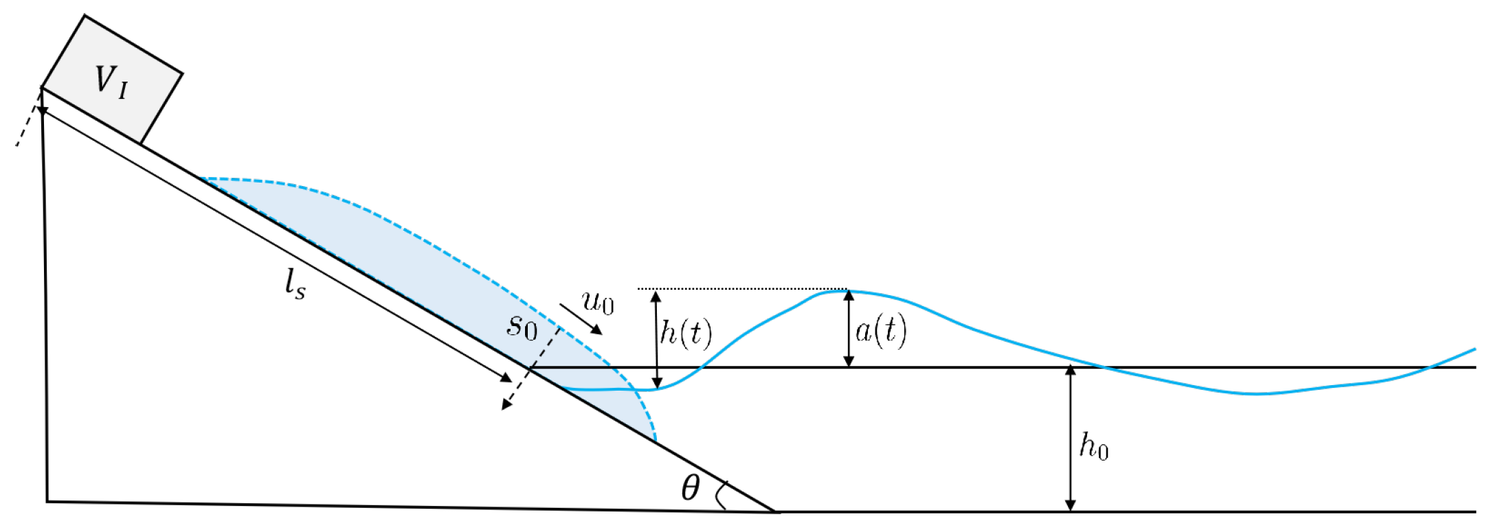
Figure 1. Physical model of landslide entering a body of water.
Jmse 13 02223 g001
Figure 2. The (a) schematic and (b) photograph of experimental facilities.
Jmse 13 02223 g002
Figure 3. High-speed camera observations. (a) t = 0 ms; (b) t = 100 ms; (c) t = 150 ms; (d) t = 200 ms; (e) t = 250 ms; (f) t = 300 ms; (g) t = 350 ms; (h) t = 400 ms.
Jmse 13 02223 g003
Figure 4. The inter-correlations among rheological parameters: (a) concentration of slide material c, consistency μ , yield stress τ c and (b) concentration of slide material c, consistency μ , flow index n.
Jmse 13 02223 g004
Figure 5. Distribution of predictor and target variables for scenario I and scenario II.
Jmse 13 02223 g005
Figure 6. Distributions of predictor variables for scenario I ( F r , S, M) and scenario II ( M i , L, B i ): (a) F r , (b) S, (c) M, (d) M i , (e) L, (f) B i .
Jmse 13 02223 g006
Figure 7. Overall data-to-model flowchart of the modeling procedure.
Jmse 13 02223 g007
Figure 8. Schematic of data clustering; points of the same color represent one cluster.
Jmse 13 02223 g008
Figure 9. The principle of gradient boosting–SHAP combined framework.
Jmse 13 02223 g009
Figure 10. Selection of optimal cluster number k for k-means in the ( F r , B i , M ) feature space.
Jmse 13 02223 g010
Figure 11. Pairwise distributions of the k-means clusters in the ( F r , B i , M ) feature space.
Jmse 13 02223 g011
Figure 12. Three-dimensional visualization of the cluster result in ( F r , B i , M ) feature space.
Jmse 13 02223 g012
Figure 13. Radar plots of evaluation metrics (a) R 2 , (b) MAE, (c) RMSE for the six prediction models.
Jmse 13 02223 g013
Figure 14. Residual distribution of the six selected prediction models: (a) gradient boosting, (b) KNN, (c) linear regression, (d) random forest, (e) SVR, (f) XGBoost.
Jmse 13 02223 g014
Figure 15. Comparison of the observed data with predicted data of gradient boosting: (a) A (scenario I); (b) A (scenario II); (c) H (scenario I); (d) H (scenario II).
Jmse 13 02223 g015
Figure 16. Mean absolute SHAP importance of each predictor variable: (a) A (scenario I), (b) H (scenario I), (c) A (scenario II), (d) H (scenario II).
Jmse 13 02223 g016
Figure 17. SHAP beeswarm distributions of each predictor variable: (a) A (scenario I), (b) H (scenario I), (c) A (scenario II), (d) H (scenario II).
Jmse 13 02223 g017
Figure 18. SHAP decision route: (a) A (scenario I), (b) H (scenario I), (c) A (scenario II), (d) H (scenario II).
Jmse 13 02223 g018
Figure 19. SHAP dependence for the top interaction pair: (a) A (scenario I), (b) H (scenario I), (c) A (scenario II), (d) H (scenario II).
Jmse 13 02223 g019
Figure 20. The 2D dependence maps for the top interaction pair: (a) A (scenario I), (b) H (scenario I), (c) A (scenario II), (d) H (scenario II).
Jmse 13 02223 g020
Table 1. Pearson correlation matrices of predictor variables for Scenario I and Scenario II.
Scenario IScenario II
FrSMMiLBi
Fr1.00−0.060.58
S−0.061.000.67
M0.580.671.00
Mi 1.000.090.57
L 0.091.00−0.26
Bi 0.57−0.261.00
Table 2. The feature interaction strengths across scenarios and targets.
ScenarioTargetRankFeature PairMean|Interaction|
scenario IA1 ( Fr , S ) 0.003003
2 ( Fr , M ) 0.001905
3 ( S , M ) 0.001823
H1 ( Fr , S ) 0.005306
2 ( Fr , M ) 0.004722
3 ( S , M ) 0.003846
scenario IIA1 ( Mi , Bi ) 0.009974
2 ( Mi , L ) 0.006596
3 ( L , Bi ) 0.005018
H1 ( Mi , Bi ) 0.014730
2 ( Mi , L ) 0.009199
3 ( L , Bi ) 0.008363
Disclaimer/Publisher’s Note: The statements, opinions and data contained in all publications are solely those of the individual author(s) and contributor(s) and not of MDPI and/or the editor(s). MDPI and/or the editor(s) disclaim responsibility for any injury to people or property resulting from any ideas, methods, instructions or products referred to in the content.