Article

Influence of Wind Direction Variability on Power Prediction in the OpenFAST with Corrected Meteorological Data


1
Department of Mechanical Engineering, Hongik University, Seoul 04066, Republic of Korea
2
Department of Mechanical and System Design Engineering, Hongik University, Seoul 04066, Republic of Korea
*
Author to whom correspondence should be addressed.
J. Mar. Sci. Eng. 2025, 13(11), 2106; https://doi.org/10.3390/jmse13112106
Submission received: 15 September 2025 / Revised: 27 October 2025 / Accepted: 29 October 2025 / Published: 5 November 2025
(This article belongs to the Special Issue Challenges of Marine Energy Development and Facilities Engineering)

Abstract

Time-varying wind conditions, on which wind turbines depend, significantly influence power generation performance. Accordingly, this study proposes an approach to improve the accuracy of wind power generation prediction by incorporating time-varying wind conditions into the OpenFAST wind turbine model. An OpenFAST wind turbine model was constructed using wind speed and wind direction data collected from the weather station near the wind farm. The numerical model was composed of cases where only wind speed was considered and cases where the time-varying wind direction was considered. And the hourly and daily power generation prediction results were compared and analyzed with the actual power generation through indicators such as correlation coefficient, RMSE (Root Mean Square Error) and NRMSE (Normalized Root Mean Square Error). As a result, in the model that reflects time-varying wind direction, errors were reduced and linear correlation was improved, both in comparison with actual power generation. Therefore, it can be concluded that this model enhances the accuracy of power generation prediction. Consequently, this study highlights the importance of considering time-varying wind direction in OpenFAST wind turbine simulation.

1. Introduction

As the global community strives to reduce its dependence on fossil fuels, pressing challenges such as climate change, environmental pollution, and resource depletion remain critical concerns. However, the rising demand for electricity has accelerated carbon emissions [1]. In this context, wind power has emerged as a promising alternative to fossil fuels and plays a pivotal role in the transition toward sustainable energy.
Wind conditions significantly affect wind turbine output, and in particular, short-term wind fluctuations can negatively impact power system operations, thereby reducing generation efficiency. In other words, the irregularity of met variables can cause instability in power generation as well as a decline in power quality within the grid [2].
To address these challenges, extensive research has focused on forecasting wind turbine power output. Accurately characterizing the relationship between wind speed variability and power generation is essential for improving predictive accuracy [3]. To this end, a wide range of forecasting methods has been explored, including statistical models, artificial neural networks, and physics-based approaches.
Statistical models can effectively reduce computational requirements and shorten processing time by directly utilizing measured wind speed data. However, their predictive accuracy decreases under rapidly changing meteorological conditions [4]. Artificial neural network-based forecasting models exploit time series meteorological inputs and turbine operational data to automatically learn nonlinear relationships and essential patterns. Nevertheless, achieving high predictive accuracy and generalization requires sufficiently large training datasets; when data are limited, prediction performance tends to deteriorate [5]. Numerical Weather Prediction (NWP) methods are widely employed to forecast wind power output using physics-based models that incorporate meteorological information and site-specific environmental characteristics such as temperature, humidity, and terrain [6]. However, these methods require strategies to quantify and reduce uncertainties in wind speed and direction data [7]. Furthermore, although Supervisory Control and Data Acquisition (SCADA) systems provide detailed information on turbine operation and status, they face limitations in terms of data availability across multiple wind farms [8].
In this study, we propose an enhanced approach for predicting wind turbine power output by incorporating temporal variations in wind direction, using wind speed and direction data obtained from met mast near a wind farm. A real wind farm was selected as the case study, and an OpenFAST wind turbine model capable of simulating actual turbine performance was developed. Power generation was estimated through numerical simulations, and the effects of wind direction variability on prediction accuracy were systematically analyzed.

2. Field Observation Data

2.1. Seongsan Wind Farm

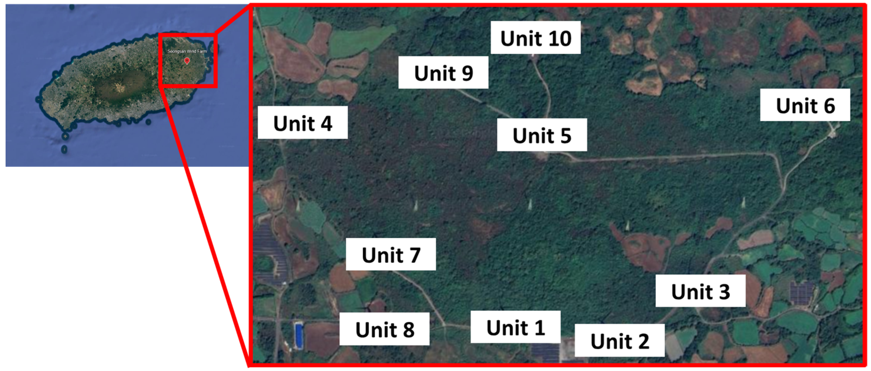
The Seongsan wind farm, situated in Jeju, Republic of Korea, comprises ten 2 MW-class wind turbines with a total installed capacity of 20 MW. The turbines are arranged as illustrated in Figure 1, and each unit employs the Vestas V80 model. A summary of the key site and turbine specifications is provided in Table 1 and Table 2.
The information on the Seongsan wind farm is provided by Korea Southern Power Co., Ltd. (Busan, Republic of Korea), and power generation as well as wind speed data can be obtained through the Public Open Data Portal [9]. In this study, daily average wind speed and power generation data (for a single turbine) and hourly power generation data (for the entire wind farm) from 2023 were utilized.

2.2. Susan Met Mast

Since the wind speed measured at the Seongsan wind farm is available only as daily averages, it has limitations in reflecting temporal variations in wind conditions. Therefore, minute-resolution wind data obtained from a nearby met mast were employed to generate input wind fields for the OpenFAST wind turbine model.
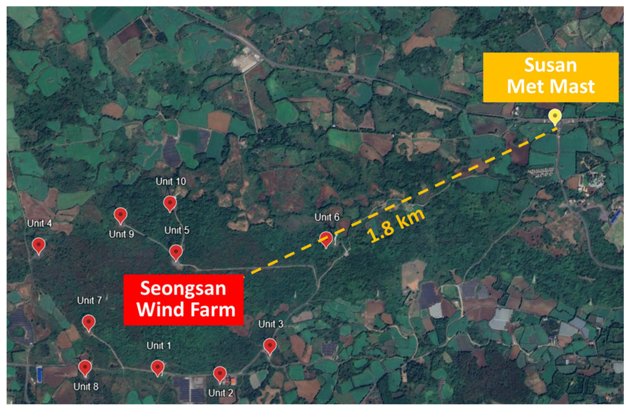
The Susan met mast is located in eastern Jeju Island, approximately 1.8 km from the Seongsan wind farm, as shown in Figure 2. Detailed information on the met mast is presented in Table 3. Through the Korea Meteorological Administration (KMA) Open Met Data Portal [10], wind speed and wind direction data measured at a reference height of 10 m above ground level were obtained. A total of 365 datasets, corresponding to the same period as the Seongsan wind farm data (Table 1), were collected.
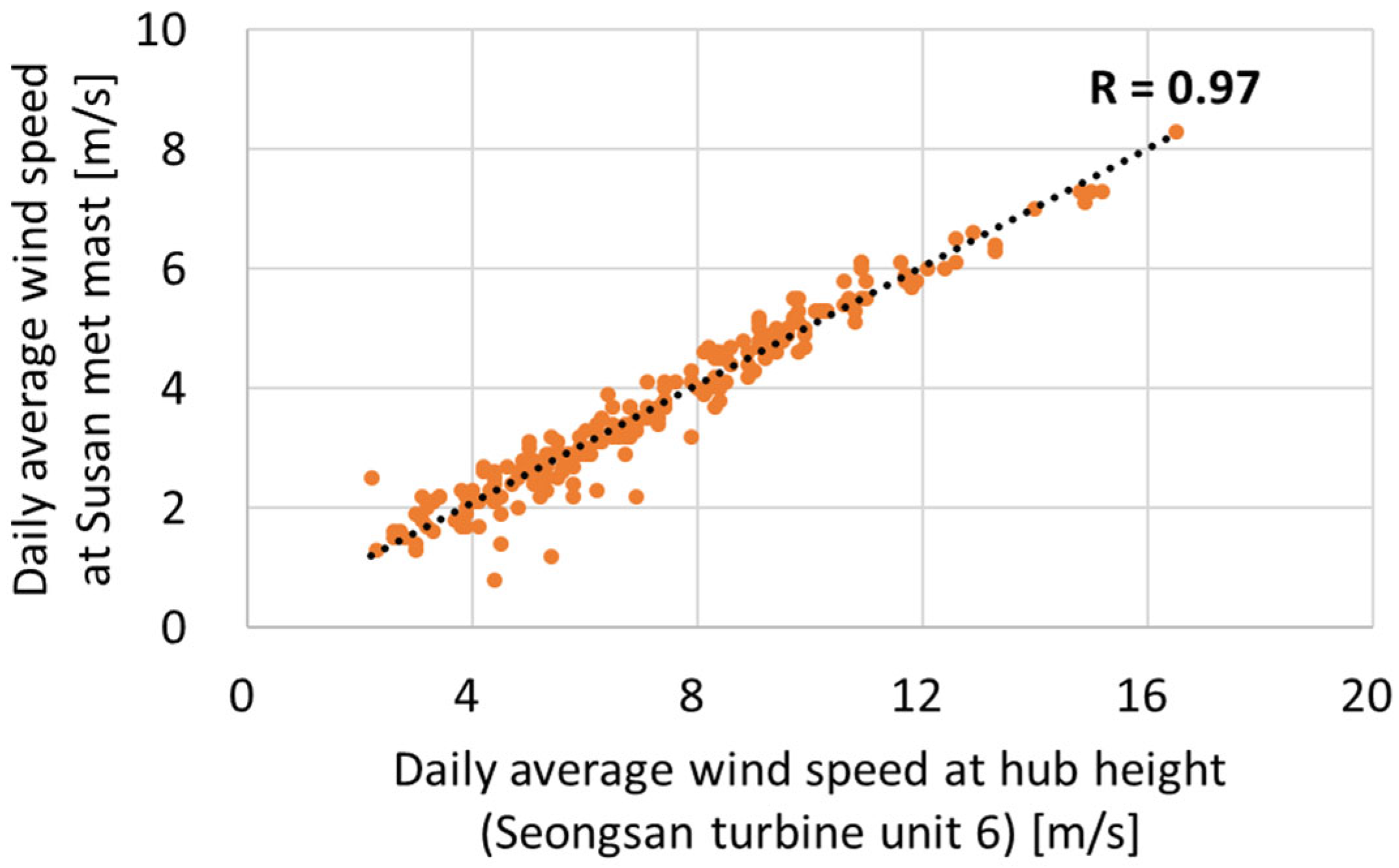
An analysis of the daily average wind speeds measured at the hub height of turbine unit 6 in the Seongsan wind farm and at the Susan met mast during the measurement periods of Table 1 and Table 3 resulted in a correlation coefficient (R) of 0.97 (Figure 3). This result indicates that the wind speeds at the two sites exhibit a strong linear relationship and similar overall variability. Therefore, after applying height-based adjustments, the wind data measured at the Susan met mast can be used as input for the simulation, which will be described in detail in Section 3.2.

3. Numerical Analysis

3.1. Numerical Model

In this study, the OpenFAST (v3.5.0) software (a coupled aero-hydro-servo-elastic analysis tool) developed by the National Renewable Energy Laboratory (NREL) was used to calculate wind turbine power output. OpenFAST performs aerodynamic analysis based on the Blade Element Momentum (BEM) theory, which assumes quasi-steady flow and may not fully capture unsteady aerodynamic effects such as dynamic stall, flow separation, and vortex-induced loads under rapidly changing wind directions. Such limitations have been discussed by Li et al. [11]. However, since the purpose of this study is to evaluate the relative influence of wind direction variability on power prediction accuracy rather than to reproduce detailed unsteady flow behavior, the BEM-based approach is considered sufficient for the intended comparative analysis.
In a theoretical sense, the variability of wind direction primarily induces yaw misalignment between the inflow and the turbine rotor axis, which directly affects the aerodynamic efficiency. The instantaneous effective wind velocity component normal to the rotor plane ( U eff ) can be expressed as
U eff = U cos γ
where U is the incoming free-stream wind speed and γ denotes the yaw misalignment angle between the wind direction and the turbine’s rotational axis. As shown in Equation (1), the effective wind speed acting on the rotor is reduced in proportion to the cosine of the yaw angle, implying that even small directional deviations diminish the aerodynamic energy available for conversion.
Since the aerodynamic power extracted by a wind turbine is proportional to the cube of the effective wind speed, the theoretical power output can be approximated by
P = 1 2 ρ A C P U eff 3 = 1 2 ρ A C P U 3 c o s 3 ( γ )
where ρ is the air density, A is the rotor swept area, and C P is the power coefficient. According to Equation (2), the c o s 3 ( γ ) term clearly indicates that even a small yaw deviation can lead to a noticeable reduction in the ideal power output. This theoretical formulation establishes the aerodynamic basis for quantifying the influence of wind direction fluctuations on power generation and justifies the incorporation of time-varying wind direction data in the OpenFAST simulation.
Since the Vestas V80 installed in the wind farm is a commercial turbine, there are limitations in constructing an OpenFAST wind turbine model that fully reflects its detailed specifications. Therefore, the widely used publicly available NREL 5 MW wind turbine model [12] was adopted to build the OpenFAST model for simulation. This model was constructed with the primary objective of analyzing and comparing output variations under changes in wind speed and direction, rather than replicating the physical characteristics of the actual turbine. Accordingly, it serves to evaluate the performance of power output predictions under varying wind conditions, rather than to provide a turbine model identical to the actual installation. The main specifications of this turbine are summarized in Table 4.
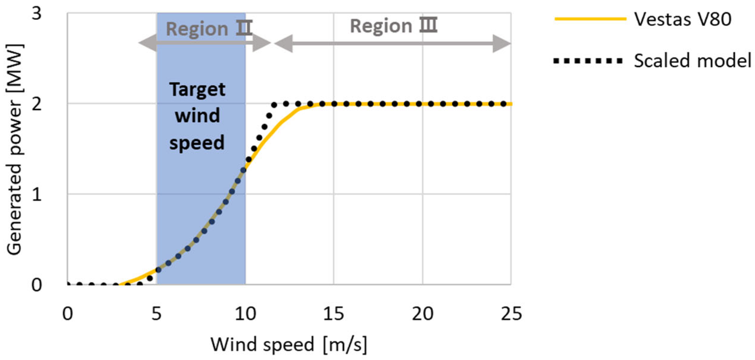
To compensate for the rated power difference between the two wind turbines, the output of the NREL 5 MW turbine was scaled, so that the OpenFAST wind turbine model could yield the same rated power as the Vestas V80. Figure 4 illustrates the power curves of the Vestas V80 (yellow solid line) and the scaled model (black dotted line). Within the cut-in to rated wind speed range (4–11.4 m/s), discrepancies can be observed between the power curves of the Vestas V80 and the scaled model. This difference occurs because, even when adjusted to have the same rated output, wind turbine performance is influenced not only by rated capacity but also by factors such as rotor diameter, aerodynamic coefficients, and control algorithms.
To conduct a detailed analysis of the effects of wind speed and wind direction on power output, this study selected days with daily average wind speeds corresponding to specific wind speed ranges. In Region II, the turbine maintains the Tip Speed Ratio (TSR) through optimal torque control, and the power output is highly sensitive to wind speed variations. In contrast, in Region III, pitch control is employed to maintain the rated power output of the turbine, thereby limiting variations in power due to changes in wind speed. Accordingly, since power output in Region II exhibits a clear dependence on wind speed being proportional to the cube of wind speed—this region was selected as the focus of analysis. Among these, wind speed ranges of 5–10 m/s, where the actual generation closely resembles the theoretical power curve, were chosen for the study (Figure 4). It should be noted that, in this study, only the wind speed range of 5–10 m/s where the scaled model and the Vestas V80 exhibit comparable power curve characteristics was used for analysis. Therefore, the discrepancy between the two models is considered negligible in terms of the relationship between wind speed and power production.

3.2. Input Wind Data

Wind shear refers to the variation of wind speed with height above the ground and can be expressed by a power-law wind speed profile, as shown in Equation (3).
V t = V × h t h α
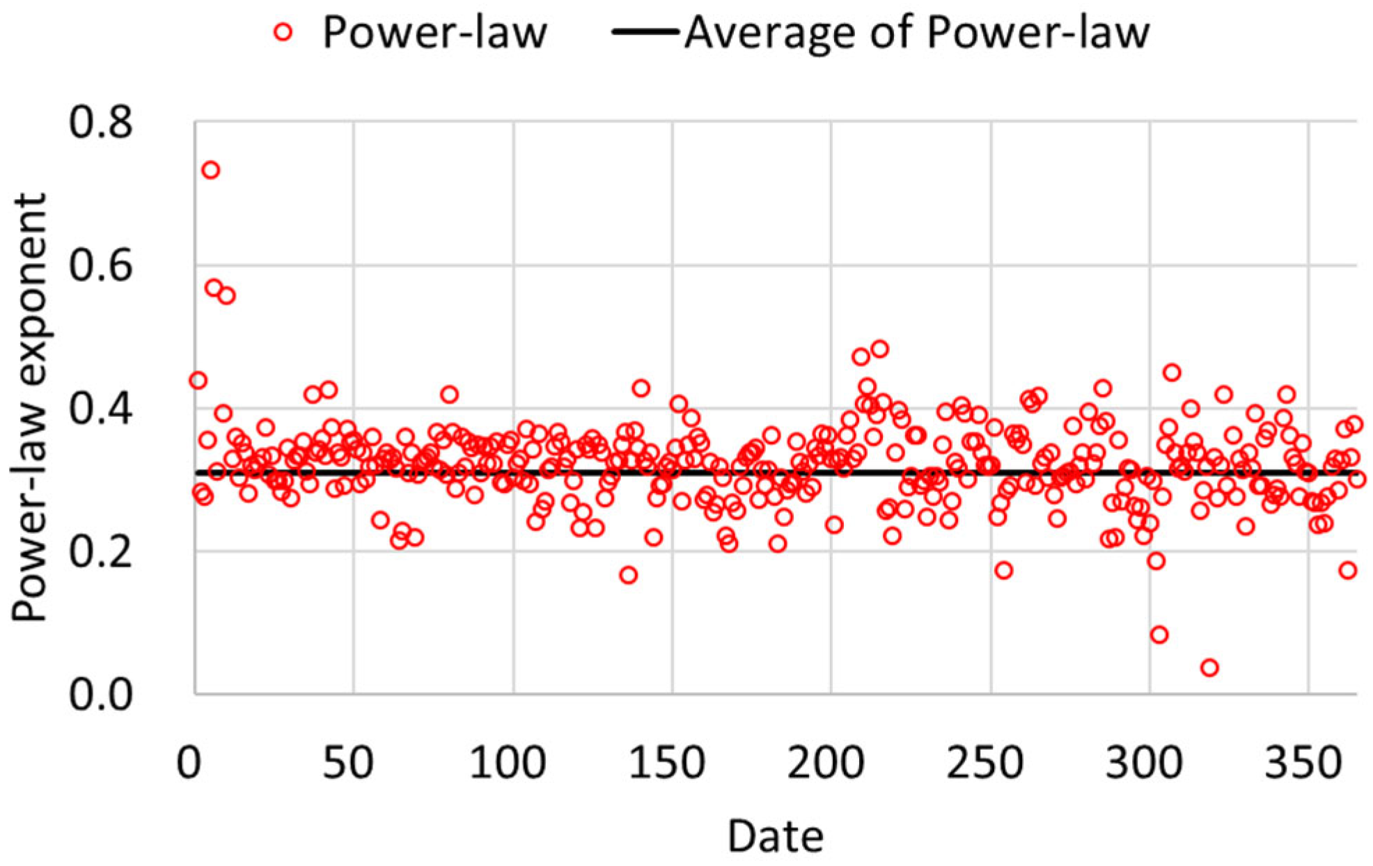
In Equation (3), h and h t denote met mast and hub heights, respectively, while V and V t are the wind speeds measured at those heights, and α indicates the power-law exponent. According to the terrain-dependent exponent table (Table 5), the power-law exponent for the mountainous Seongsan area is 0.30. To verify the suitability of this value, the exponent was calculated using wind speed data measured at the Susan met mast ( V ) and at the hub height of Seongsan turbine unit 6 ( V t ). A total of 365 daily exponents were derived for the year 2023 (Figure 5), yielding an average exponent of approximately 0.30, consistent with the terrain-based reference value. Therefore, in this study, a power-law exponent of 0.30 was applied to adjust wind speeds with respect to height.
Table 6 summarizes the results of the error and correlation analysis between the daily average wind speed data measured at the Susan met mast and at Seongsan turbine unit 6. A comparison of the Root Mean Square Error (RMSE) and the Normalized Root Mean Square Error (NRMSE) before and after height correction showed reductions of 2.9 m/s and 19.98 percentage points, respectively, with only a small error of 0.79 m/s relative to Seongsan turbine unit 6. Therefore, in this study, the wind speed data from Susan met mast were height-corrected and subsequently used as input wind data for the OpenFAST model.
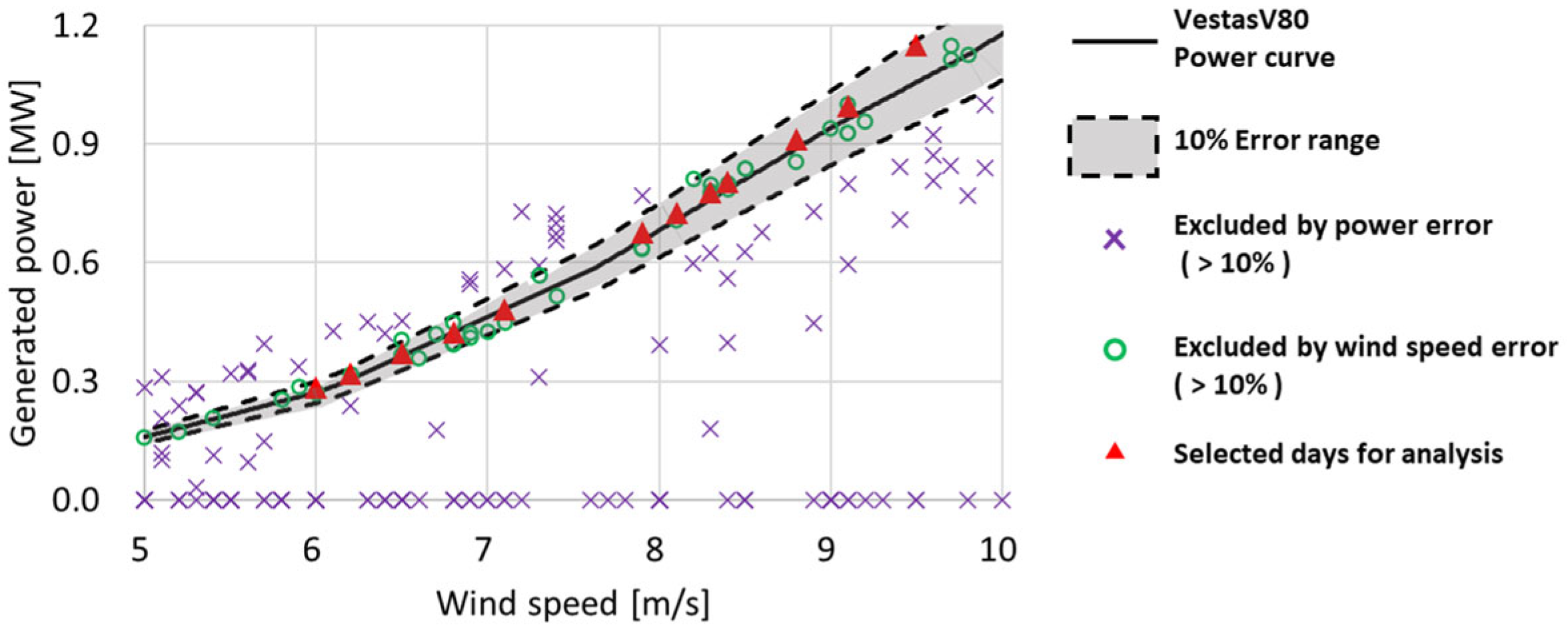
Actual power generation does not always coincide with the ideal power curve for a given wind speed. Figure 6 presents a comparison between the measured wind speed and actual power output of Seongsan turbine unit 6 (scatter plot) and the theoretical power curve (black solid line). While most of the generation values are distributed near the power curve, abnormally low values, including those close to 0 MW, were also observed. These anomalies are presumed to result from temporary turbine shutdowns, mechanical malfunctions, or interventions by the control system.
When data affected by external factors are included, it becomes difficult to accurately determine the relationship between wind speed and power generation. Therefore, to ensure the reliability of the analysis, days were excluded if the error between the actual power output and the theoretical power curve exceeded 10%, or if the difference between the hub-height adjusted wind speed from Susan met mast and the wind speed measured at Seongsan turbine unit 6 exceeded 10%. Based on these criteria, a total of 12 days were selected for analysis, and the corresponding information is presented in Table 7.

3.3. Analysis Cases

In constructing the OpenFAST wind turbine model, nacelle yaw control was not considered. Instead, the impact of wind direction variability on power prediction was examined by analyzing the differences in power generation between cases with and without wind direction adjustments relative to the prevailing wind. For this purpose, two analysis cases were defined, as summarized in Table 8.
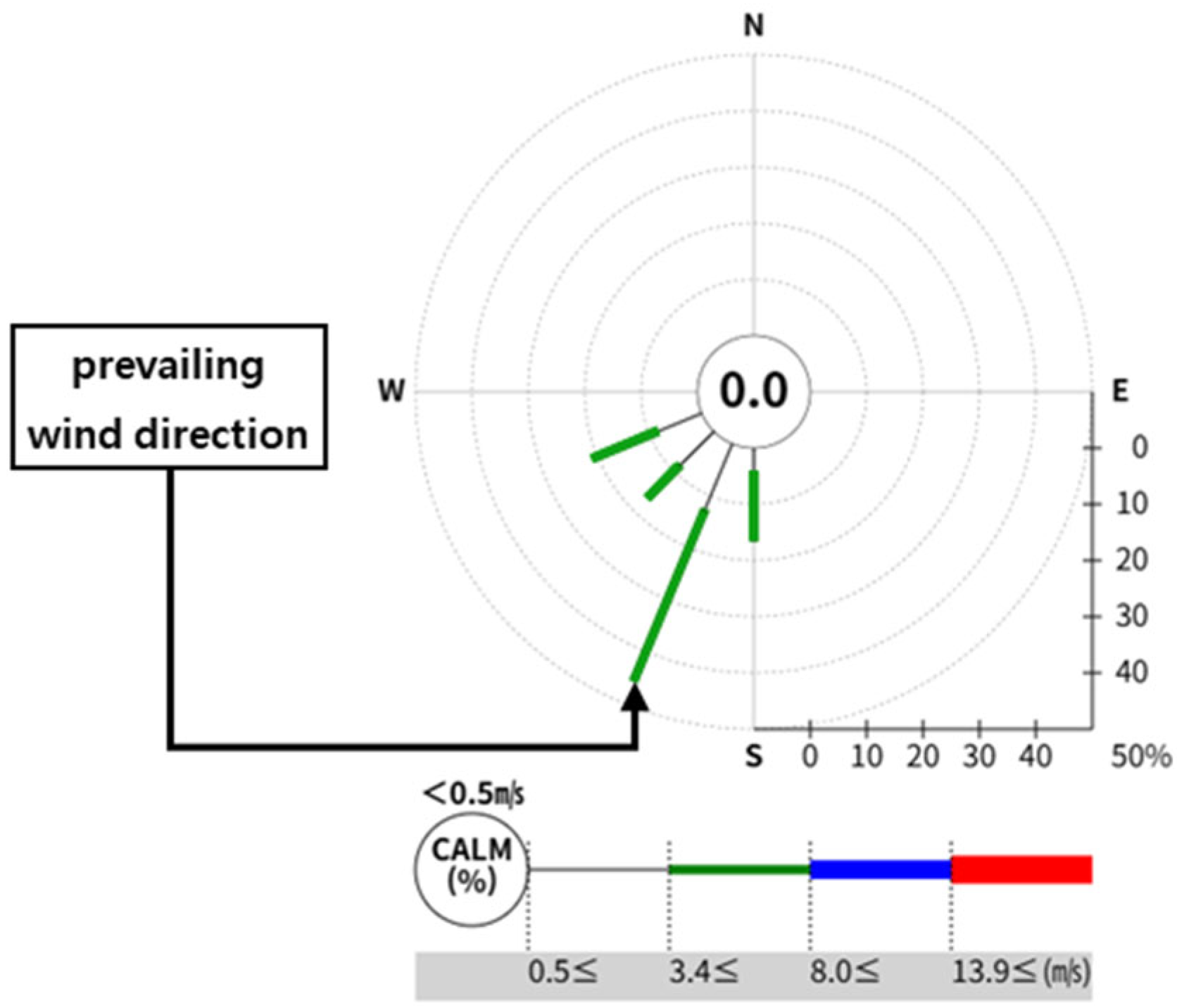
Since yaw control was not considered in the OpenFAST wind turbine model, the turbine was aligned each day to face the prevailing wind direction. The prevailing wind direction for each day was determined using wind rose data from the Susan met mast, provided by the Korea Meteorological Administration (KMA) Open Met Data Portal [10]. For instance, on 28 April, the most frequent wind direction observed in the wind rose (Figure 7) was 202.5°, which was applied as the prevailing wind direction. Accordingly, Case 1 assumes a constant wind direction aligned with the turbine, such that the wind always comes from the prevailing direction, while Case 2 incorporates hourly variations in wind direction relative to the prevailing wind.
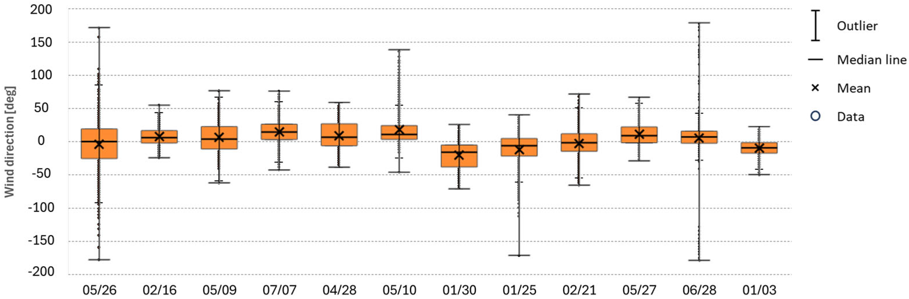
Figure 8 presents box plots of wind-direction deviation (∆γ) for the 12 selected days, referenced to each day’s prevailing direction (0°). The boxes represent the interquartile range (IQR), spanning the 25th to 75th percentiles, and the solid line inside each box denotes the median values. A median line close to 0 indicates that hourly directions converge well to the prevailing direction, whereas a taller box (larger IQR) denotes greater variability. The solid lines at the ends of the line indicate the maximum and minimum value and the “x” mark inside each box denotes mean values.
In Figure 8, 26 May shows the greatest wind-direction variability, as indicated by the tallest box (largest interquartile range). In contrast, 30 January shows a median notably offset from 0 , implying a systematic bias away from the prevailing direction. This behavior is consistent with the sector boundary effect. Since wind roses typically use sectors ranging from 0 to 22.5°, defining the dominant direction as the central angle of the most frequent sector can lead to non-zero central deviations when observations are distributed near one edge of that sector.

4. Results and Discussion

To analyze the linear relationship between the OpenFAST wind turbine model and the actual turbine output, the correlation coefficient (R), representing the degree of linear correlation between two variables, was employed and calculated as shown in Equation (4). In addition, the Root Mean Square Error (RMSE) given in Equation (5) was computed to quantitatively compare the magnitude of errors, while the Normalized Root Mean Square Error (NRMSE) in Equation (6) was used to evaluate the errors relative to the rated capacity.
R = ( X X ¯ ) ( Y Y ¯ ) ( X X ¯ ) 2 ( Y Y ) ¯ 2
R M S E = 1 N × i = 1 N ( X i Y i ) 2
N R M S E = 1 N × i = 1 N ( X i Y i ) 2 P R a t e d × 100
In Equations (4)–(6), X denotes the output of the OpenFAST wind turbine model, while Y represents the actual turbine output; X ¯ and Y ¯ indicate the average values of the respective turbine outputs. P R a t e d corresponds to the installed capacity of both the wind farm and a single wind turbine. In Section 4.1, the simulated hourly power generation of the wind farm is compared with the measured data, whereas in Section 4.2, the simulated daily generation of Seongsan turbine unit 6 (a single turbine) is compared with the corresponding actual measurements.

4.1. Comparison of Hourly Power Generation (Seongsan Wind Farm)

The hourly power generation of a wind farm is calculated as the sum of the individual outputs of the ten turbines within the site. Since the OpenFAST wind turbine model used in this study represents a single turbine, a scaling process was required to scale the simulation results to the wind farm level for comparison. This was applied as expressed in Equation (7), and the results were compared with the actual wind farm generation.
P ^ t = N = 1 10 P × ( P t u n i t . N P t u n i t . R e f )
Since each turbine within the wind farm generates a different amount of power, it is not appropriate to directly compare the Seongsan wind farm power with the simulation results simply by multiplying the simulated single turbine output ( P ^ t ) by the number of turbines. However, to examine the trend of power variation over time, the wind farm generation was estimated from the simulation results as follows. The ratio of the daily power of each turbine ( P t u n i t . N ) ) to that of the reference turbine ( P t u n i t . R e f ) was applied to the OpenFAST model output and the total wind farm output was then obtained by summing the outputs of all ten turbines. Turbine unit 6, located closest to met mast, was selected as the reference turbine. Using the input wind data for 12 days, OpenFAST simulations were performed for each analysis case, and the wind farm generation was subsequently calculated based on the daily output ratios ( P t u n i t . N / P t u n i t . R e f ) relative to the reference turbine.
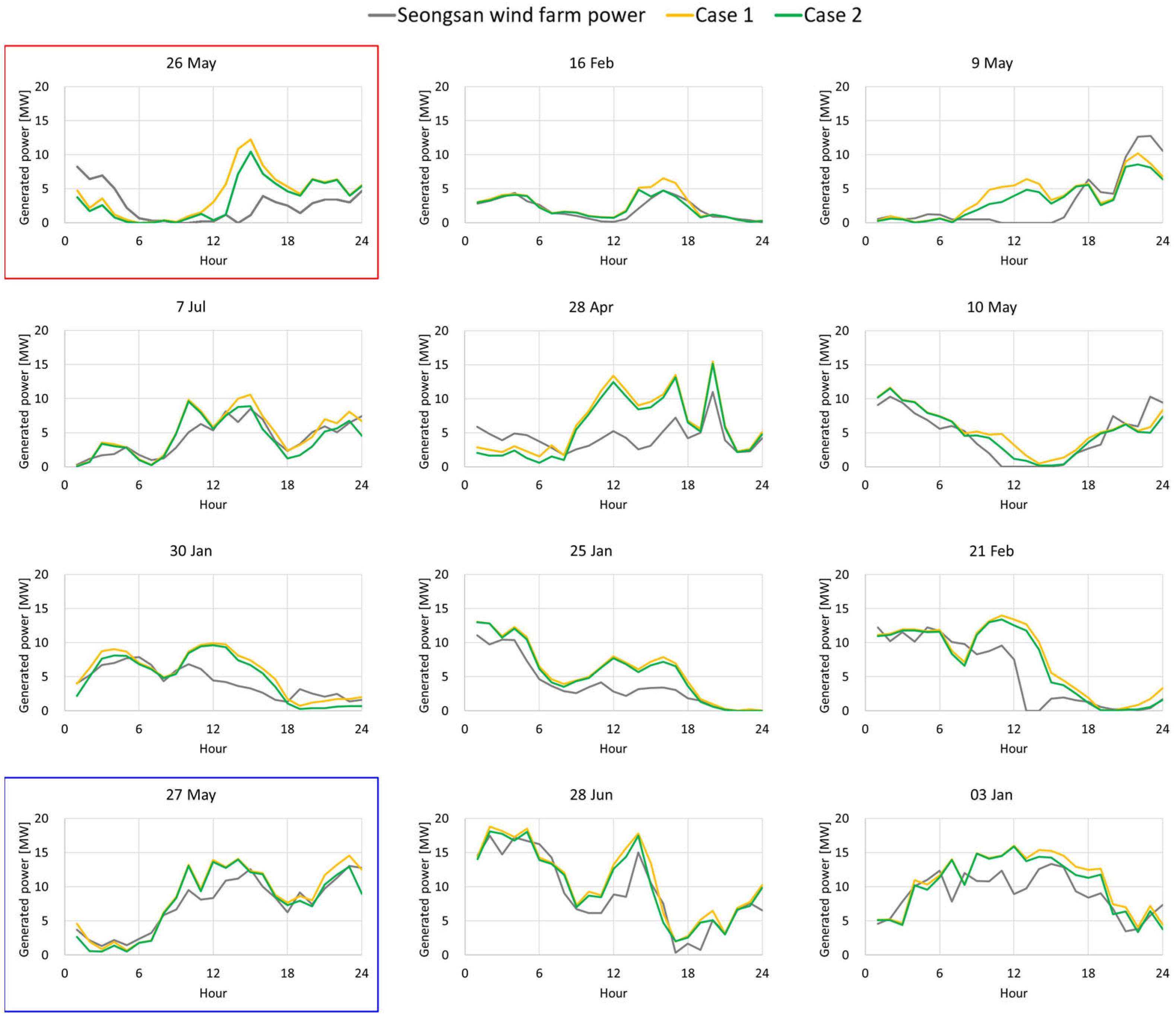
The simulated and actual hourly power generation values are presented in Figure 9, while the correlation coefficient (R), RMSE, and NRMSE calculated using Equations (5) and (6) are compared in Table 9.
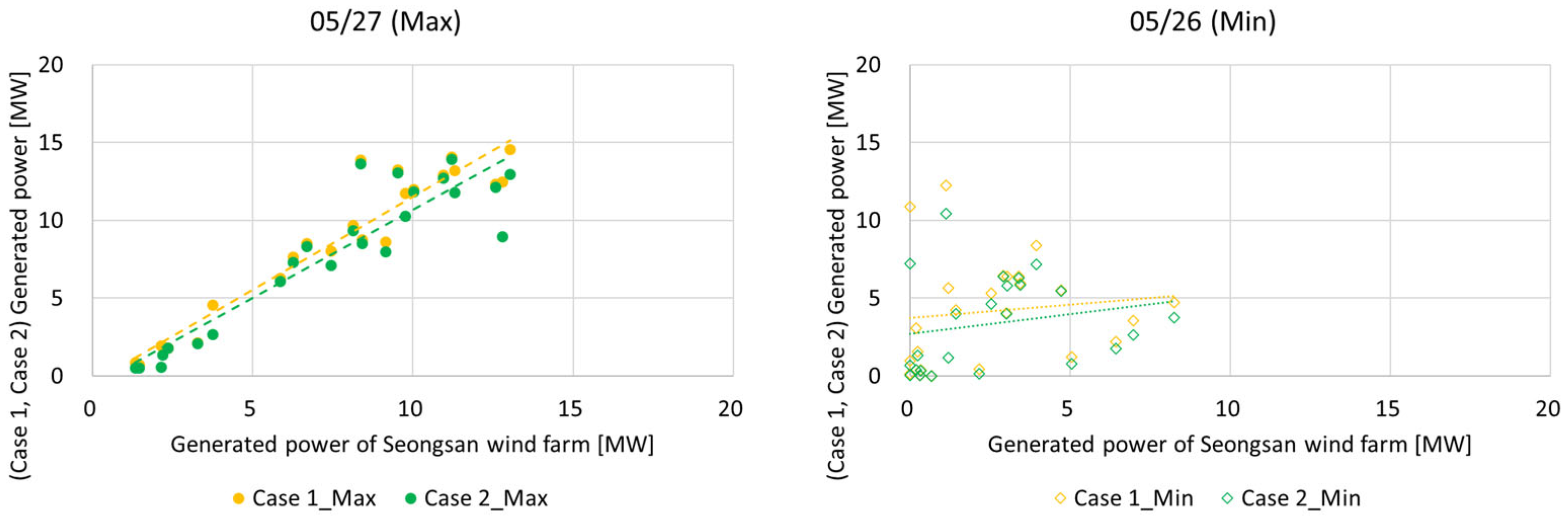
Although the power generation trends of the actual wind farm and the OpenFAST wind turbine model were similar in some cases, discrepancies were observed on certain days. This is considered to be due to the expansion of wind farm output based on the wind speed and power data of Seongsan turbine unit 6, which limits the ability to capture the unique output characteristics of each turbine. Furthermore, since the turbine outputs used in Equation (7) were daily totals, variations in hourly output could not be considered, which is also believed to have contributed to the differences. As shown in Table 9, on 27 May the correlation coefficient (R) was very high, with values of 0.96 and 0.92, indicating a strong linear relationship. In contrast, on 26 May, the coefficients were low at 0.12 and 0.21. To further analyze this, Figure 10 compares the hourly generation for these two dates using scatter plots with trend lines. When R was lowest (26 May), the hourly output data were widely dispersed around the trend line, indicating a weak correlation between simulation and actual generation. This discrepancy primarily results from the aggregation of farm-level power output derived from a single turbine (Seongsan turbine unit 6), which introduces scaling uncertainty and limits the model’s ability to represent the spatial variability among turbines. Conversely, when R was highest (27 May), the data were concentrated near the trend line, demonstrating a strong correlation between the two outputs.
While R indicates the similarity of variations, it does not reflect the magnitude of absolute errors. Therefore, RMSE and NRMSE were compared across cases using the results in Table 9 to quantitatively evaluate the errors. Case 2 consistently showed lower errors than Case 1 across all dates, suggesting that accounting for wind direction variability contributed to improved accuracy. Case 2, which incorporates temporal changes in wind direction, better represents actual operating conditions, thereby reducing discrepancies from the measured power generation.
The consistent reduction in RMSE and NRMSE observed in Case 2 can be analytically explained by the effect of yaw misalignment. When wind direction varies with time, the effective power coefficient decreases according to the relationship shown in Equation (8):
P P 0 = c o s 3 γ ( t )
where P 0 represents the idealized power under zero yaw. This relation implies that the energy capture ratio decreases nonlinearly with increasing yaw misalignment, confirming that temporal wind direction variability must be considered to achieve physically accurate simulation results. In this study, this wind direction variability is quantified through a wind direction variability factor based on the instantaneous yaw misalignment, c o s 3 γ ( t ) , which serves as a correction term applied to the idealized power.
The OpenFAST model in Case 2, which dynamically updates γ with measured met mast data, reflects this theoretical dependency and thus reproduces the observed attenuation in power output. The analytical consistency between simulated and measured results substantiates that the model improvement is not merely empirical but grounded in aerodynamic principles.
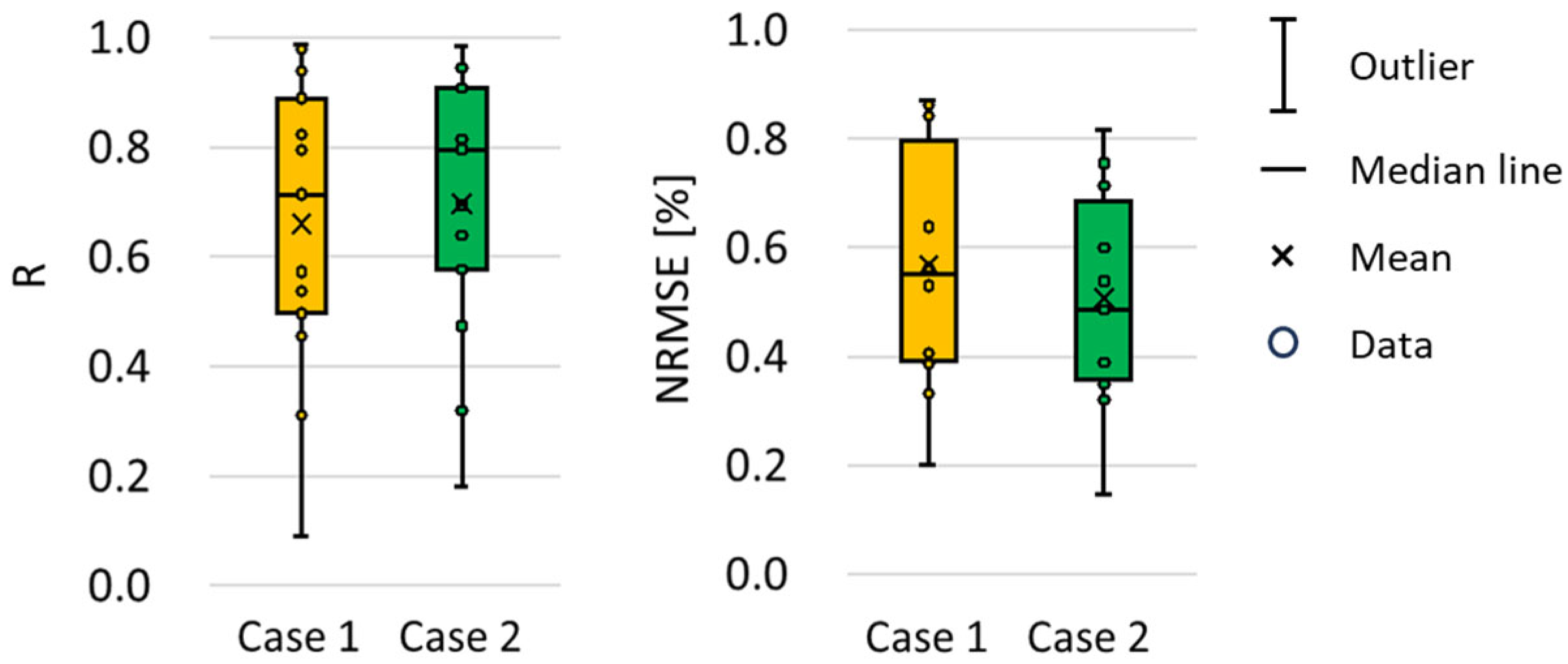
Figure 11 presents box plots of R and NRMSE for the 12 selected days. In the R graph, Case 2 shows higher median and mean values than Case 1, indicating an overall stronger linear correlation. In the NRMSE graph, Case 2 exhibits lower median and mean values as well as a smaller interquartile range (IQR) compared to Case 1.

4.2. Daily Power Generation Comparison (Seongsan Turbine Unit 6)

Section 4.2 analyzes the effect of wind direction variability on simulated power generation for a single turbine (Seongsan turbine unit 6). For the dates selected in Section 3.2, simulations were conducted for each analysis case to calculate the daily power generation.
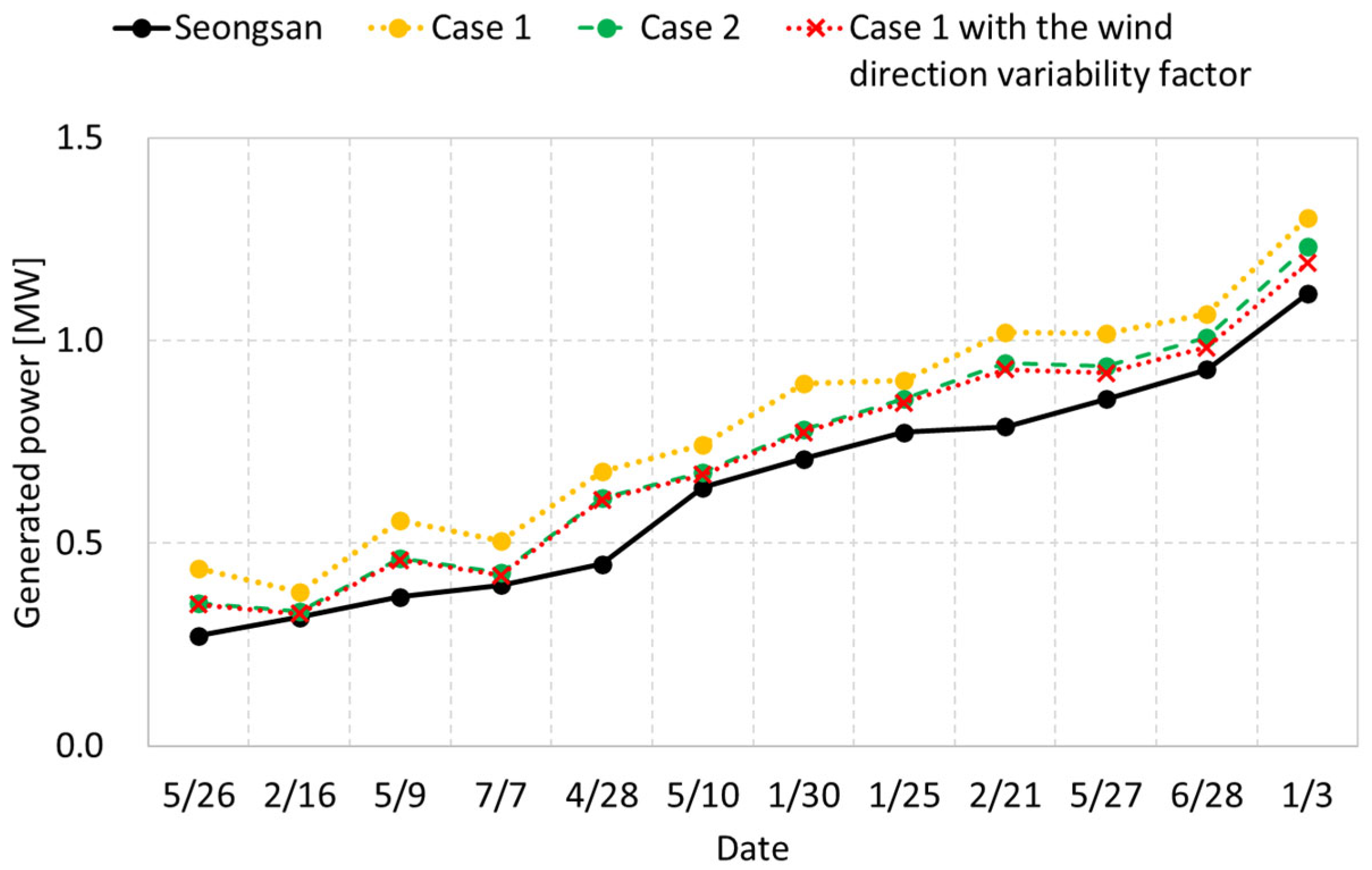
Figure 12 and Table 10 compare the measured daily generation at Seongsan with the model outputs. The black line shows Seongsan (measurements), the yellow dotted line shows Case 1, the green line shows Case 2, and the red dashed line with × markers shows Case 1 with the wind direction variability factor. With the nacelle yaw held fixed, temporal wind direction variability directly manifests as a time-varying yaw misalignment γ ( t ) between the inflow and the rotor axis. Because aerodynamic power scales approximately as P = P 0 c o s 3 γ ( t ) , this variability reduces the expected output. Consistent with this mechanism, Case 1 corrected by the wind direction variability factor ( c o s 3 γ ( t ) ) closely matches with Case 2 (Figure 12; Table 10). This correspondence indicates that the numerical model effectively captures yaw misalignment losses, and that a simple multiplicative correction to Case 1 reproduces the same effect.
t = 1 n i = 1 n ( A i Y i B i Y i ) i = 1 n A i Y i B i Y i d ¯ 2 n 1 n
p = 2 1 F t ( t ; n 1 )
The t and p values in Table 11 were calculated according to Equations (9) and (10), representing the results of a paired t-test used to verify the statistical significance of the prediction error differences between Case 1 and Case 2. The predicted power outputs of each case were denoted as A i and B i , respectively, while the measured power at Seongsan was denoted as Y i . To compare the predictive accuracy of the two models, the absolute errors A i Y i and B i Y i were computed, and their mean ( d ¯ ) and standard deviation of the daily error differences were used to calculate the t statistic, as expressed in Equation (9). The corresponding p value was obtained through the cumulative integration of the t-distribution function that includes the Gamma function, as defined in Equation (10). As shown in Table 11, the computed p = 3.55 × 10⁻⁸ (<0.001) and t = 13.46 confirm that the difference between the two cases is statistically significant, indicating that cumulative integration of the t-distribution function that includes the Gamma function.
Table 11 presents the values of R, RMSE, and NRMSE for the daily power generation results of the two analysis cases. Since the comparison in Section 4.2 was conducted for a single turbine, the resulting R values were higher than those obtained for the wind farm in Section 4.1. Meanwhile, Case 2 exhibited lower errors in terms of both RMSE and NRMSE compared to Case 1.
Variations in wind direction alter the effective inflow and blade angle of attack; therefore, Case 1, which idealizes the wind as always perpendicular to the rotor plane, tends to overestimate power. Case 2, which incorporates temporal changes in wind direction, yields lower errors. Table 11 quantifies this: while all approaches correlate equally with measurements, the error magnitudes decrease from Case 1 to Case 2 and to Case 1 with the wind direction variability factor. Paired t-tests on daily absolute-error differences show that both Case 2 and the wind direction variability adjusted in Case 1 significantly improve upon Case 1. Moreover, the close agreement between Case 2 and the corrected Case 1 (with the wind direction variability factor) shows that Case 2 properly reflects the effect of yaw misalignment losses; taken together, these results validate Case 2 as a sound and reliable approach for power prediction under wind direction variability.
To validate the significance of these errors, the prediction error rate was evaluated based on the Korea Power Exchange (KPX) power generation prediction system [14]. Under this system, settlement payments are adjusted according to the error rate between forecasted and actual generation, with errors within ±8% generally regarded as acceptable. The NRMSE derived in Case 2 (4.73%) was found to be well within this acceptable threshold. Therefore, it can be concluded that incorporating wind direction variability enables simulation-based wind turbine power predictions to be sufficiently reliable for practical operational applications.

5. Conclusions

In this study, wind turbine power generation was predicted using numerical simulations with the OpenFAST wind turbine model. Actual wind measurements from Susan met mast were employed to analyze the predictive performance of wind turbine generation under varying wind directions. To this end, an OpenFAST wind turbine model capable of numerically simulating turbine power output was developed, and wind speed and direction data were obtained from a met mast in close proximity to the wind farm.
The predictive performance of two models, one without wind direction variability (Case 1) and one with wind direction variability (Case 2), was compared using hourly power generation. The results showed that Case 2 achieved an average increase of 1.38% in the correlation coefficient (R) and an average reduction of 12.82% in normalized root mean square error (NRMSE) compared to Case 1. Since Case 1 assumes the idealized condition of wind always impinging perpendicularly on the rotor plane, it tended to overestimate actual power generation. By contrast, Case 2 partially accounted for temporal variations in the angle of incidence and the resulting reduction in relative wind speed, thereby providing a more realistic representation of actual operating conditions. Consequently, it was confirmed that incorporating wind direction variability leads to simulation results more closely aligned with measured power generation.
From a theoretical perspective, the improvement in predictive accuracy achieved by considering wind direction variability originates from the fundamental c o s 3 ( γ ) dependency between yaw angle and aerodynamic power extraction, as described in Equation (8). This relationship directly links temporal fluctuations in inflow direction to reductions in effective wind speed ( U eff = U c o s ( γ ) ) and aerodynamic power coefficient ( C P ). By incorporating this physical relationship, the OpenFAST model reproduces the actual aerodynamic response of the turbine more accurately, confirming that the observed improvements are theoretically consistent with the physics of wind energy conversion.
In summary, considering temporal wind direction variability in the OpenFAST simulation significantly improves the accuracy of wind power prediction. By utilizing meteorological measurements rather than static or purely statistical assumptions, this study presents a practical and physically grounded approach for enhancing simulation-based power forecasting. Future work will extend the model to include turbine control characteristics and grid effects and expand validation using long-term and seasonal datasets to further improve predictive robustness.

Author Contributions

Conceptualization, D.I. and Y.L.; methodology, D.I. and Y.L.; software, D.I.; validation, Y.L. and Y.H.B.; formal analysis, D.I.; investigation, D.I.; resources, Y.H.B.; data curation, Y.H.B.; writing—original draft preparation, D.I.; writing—review and editing, Y.L. and Y.H.B.; visualization, D.I.; supervision, Y.H.B.; project administration, Y.H.B.; funding acquisition, Y.H.B. All authors have read and agreed to the published version of the manuscript.

Funding

This research was funded by the Korea Institute of Marine Science & Technology Promotion (KIMST), funded by the Ministry of Oceans and Fisheries (MOF), Republic of Korea (RS-2022-KS221682).

Institutional Review Board Statement

Not applicable.

Informed Consent Statement

Not applicable.

Data Availability Statement

The original contributions presented in this study are included in the article. Further inquiries can be directed to the corresponding author.

Conflicts of Interest

The authors declare no conflicts of interest.

References

  1. Perez-Sanjines, F.; Peeters, C.; Verstraeten, T.; Antoni, J.; Nowé, A.; Helsen, J. Fleet-based early fault detection of wind turbine gearboxes using physics-informed deep learning based on cyclic spectral coherence. Mech. Syst. Signal Process. 2023, 185, 109760. [Google Scholar] [CrossRef] [Scilit]
  2. Choi, J.; Choi, H. Prediction of wind power generation using deep learning. J. Korea Inst. Electron. Commun. Sci. 2021, 16, 329–338. [Google Scholar]
  3. Lee, H.; Kim, K.; Jeong, H.; Lee, H.; Kim, H.; Park, J. A study on wind power forecasting using LSTM method. Trans. Korean Inst. Electr. Eng. 2020, 69, 1157–1164. (In Korean) [Google Scholar] [CrossRef] [Scilit]
  4. Perr-Sauer, J.; Tripp, C.; Optis, M.; King, J. Short-term wind forecasting using statistical models with a fully observable wind flow. J. Phys. Conf. Ser. 2020, 1452, 012083. [Google Scholar] [CrossRef] [Scilit]
  5. Zhang, G.; Patuwo, B.E.; Hu, M.Y. Forecasting with artificial neural networks: The state of the art. Int. J. Forecast. 1998, 14, 35–62. [Google Scholar] [CrossRef] [Scilit]
  6. Negnevitsky, M.; Potter, C.W. Innovative short-term wind generation prediction techniques. In Proceedings of the 2006 IEEE PES Power Systems Conference and Exposition, Atlanta, GA, USA, 29 October–1 November 2006; IEEE: Piscataway, NJ, USA, 2006; pp. 60–65. [Google Scholar]
  7. Al-Yahyai, S.; Charabi, Y.; Al-Badi, A.; Gastli, A. Nested ensemble NWP approach for wind energy assessment. Renew. Energy 2012, 37, 150–160. [Google Scholar] [CrossRef] [Scilit]
  8. Kang, J.; Sobral, J.; Soares, C.G. Review of condition-based maintenance strategies for offshore wind energy. J. Mar. Sci. Appl. 2019, 18, 1–16. [Google Scholar] [CrossRef] [Scilit]
  9. Ministry of the Interior and Safety (MOIS). Available online: https://www.data.go.kr/index.do (accessed on 31 December 2024).
  10. Korea Meteorological Administration (KMA). Jeju Observatory Information. Available online: https://www.kma.go.kr/ (accessed on 31 December 2024).
  11. Li, T.; Zhang, Y.; Yang, Q.; Zhou, X.; Zhang, Z.; Wang, T. Unsteady aerodynamic characteristics of a floating offshore wind turbine in propeller state. Renew. Energy 2025, 246, 122861. [Google Scholar] [CrossRef] [Scilit]
  12. Jonkman, J.; Butterfield, S.; Musial, W.; Scott, G. Definition of a 5-MW Reference Wind Turbine for Offshore System Development; Technical Report No. NREL/TP-500-38060; National Renewable Energy Laboratory: Golden, CO, USA, 2009. [Google Scholar]
  13. Ray, M.L.; Rogers, A.L.; McGowan, J.G. Analysis of Wind Shear Models and Trends in Different Terrains; Technical Report; Renewable Energy Research Laboratory, Department of Mechanical and Industrial Engineering, University of Massachusetts: Amherst, MA, USA, 2006. [Google Scholar]
  14. Korea Power Exchange (KPX). Electricity Market Operation Rules; Korea Power Exchange: Seoul, Republic of Korea, 2025; p. 469. (In Korean) [Google Scholar]
Figure 1. Layout of wind turbines in Seongsan wind farm.
Jmse 13 02106 g001
Figure 2. Distance between Seongsan wind farm and Susan met mast.
Jmse 13 02106 g002
Figure 3. Correlation between daily average wind speeds measured at Seongsan turbine unit 6 and at Susan met mast (dashed lines: linear trendlines of wind velocity between Seongsan turbine unit 6 and Susan met mast).
Jmse 13 02106 g003
Figure 4. Power curve of Vestas V80 and scaled model.
Jmse 13 02106 g004
Figure 5. Daily power-law exponent between Susan met mast and Seongsan turbine unit 6.
Jmse 13 02106 g005
Figure 6. Comparison between generated power curve.
Jmse 13 02106 g006
Figure 7. Wind rose diagram for 28 April 2023.
Jmse 13 02106 g007
Figure 8. Wind directional deviation for each analyzed day.
Jmse 13 02106 g008
Figure 9. Comparison of simulated and actual hourly generated power (red box: lowest daily correlation and minimum R; blue box: highest daily correlation and maximum R).
Jmse 13 02106 g009
Figure 10. Generated power at maximum and minimum R (dashed lines: linear trendlines of power output between the Seongsan wind farm and each case).
Jmse 13 02106 g010
Figure 11. Comparison of R and NRMSE of generated power.
Jmse 13 02106 g011
Figure 12. Comparison of daily generated power.
Jmse 13 02106 g012
Table 1. Summary of site information and measurement intervals at Seongsan wind farm.
DescriptionValue
LocationN 33°26′40″ E 126°49′57″
Altitude [m]162
Measurement height, h [m]78
Measurement period1 January 2023–31 December 2023 (1 year)
Data time intervalWind farm power1 h
Each unit turbine
power and wind speed
1 day
Table 2. Description of turbine model at Seongsan wind farm.
DescriptionValue
Wind turbine modelVestas V80
Rated   power ,   P t [MW]2.0
Cut-in wind speed [m/s]4
Rated wind speed [m/s]15
Cut-out wind speed [m/s]25
Table 3. Description of Susan met mast.
DescriptionValue
LocationN 33° 27′00″ E 126° 51′04″
Altitude [m]102
Measurement height, h [m]10
Measurement period1 January 2023–31 December 2023 (1 year)
Data time intervalWind speed1 day
(for estimation of power-law exponent)
Wind speed and direction1 min
(for power calculation)
Table 4. Description of NREL 5 MW reference wind turbine.
DescriptionValue
ModelNREL 5 MW
Rated power, P [MW]5.0
Hub height, h [m]90
Cut-in wind speed [m/s]3
Rated wind speed [m/s]11.4
Cut-out wind speed [m/s]25
Table 5. Typical power-law exponents for varying terrain [13].
Terrain DescriptionPower-Law Exponent, α
Smooth, hard ground, lake or ocean0.10
Short grass on untilled ground0.14
Tall row crops, hedges, a few trees0.20
Many trees and occasional buildings0.22–0.24
Wooded country, small towns and suburbs0.28–0.30
Urban areas with tall buildings0.4
Table 6. Quantitative comparison of daily wind speed.
DescriptionSeongsan
Turbine Unit 6
Susan
Met Mast
Extrapolated
Wind Speed
Ref. height [m]781078
R-0.970.97
RMSE [m/s]-3.690.79
NRMSE [%]-25.285.30
Table 7. Wind speed and power errors for the 12 selected days.
Date26 May16 Feb9 May7 Jul28 Apr10 May30 Jan25 Jan21 Feb27 May28 Jun3 Jan
Wind speed [m/s]Seongsan
turbine unit 6
6.006.206.506.807.107.908.108.308.408.809.109.50
Extrapolated
wind speed
6.116.306.856.857.597.968.528.338.528.899.2610.19
Error [%]1.861.565.420.776.940.805.170.411.421.021.764.00
Generated power [MW]Seongsan
turbine unit 6
0.2720.3170.3670.3970.4480.6370.7080.7740.7870.8550.9281.115
Estimated power
(using power curve)
0.2850.3200.3720.4240.4830.6770.7270.7800.8060.9110.9971.192
Error [%]4.780.831.276.767.866.302.690.792.356.557.456.90
Table 8. Analysis cases.
Case #Wind Direction
Case 1Fixed wind direction
(Same wind direction depending on time)
Case 2Considering wind direction variation
(Wind direction changing with time)
Table 9. Daily R, RMSE, and NRMSE values for hourly generated power.
Date26 May16 Feb9 May7 Jul28 Apr10 May30 Jan25 Jan21 Feb27 May28 Jun3 Jan
R
[-]
Case 10.120.900.710.910.560.870.710.920.750.960.920.77
Case 20.210.890.800.840.560.890.730.930.780.920.920.75
RMSE
[MW]
Case 10.1720.0410.1280.0670.1740.0820.1060.1080.1680.0780.1130.131
Case 20.1430.0300.1080.0650.1630.0700.0980.0970.1510.0770.0970.120
NRMSE
[%]
Case 10.8600.2050.6390.3350.8700.4080.5310.5410.8410.3910.5640.654
Case 20.7140.1510.5390.3230.8170.3500.4880.4870.7550.3870.4870.601
Table 10. Comparison of daily generated power by average wind speed.
DateSeongsan
Turbine Unit 6 [MW]
Case 1
[MW]
Case 2
[MW]
Case 1 with
Wind Direction Variability Factor
[MW]
26 May0.272 0.437 0.351 0.349
16 Feb0.317 0.380 0.331 0.326
9 May0.367 0.555 0.463 0.458
7 Jul0.397 0.505 0.427 0.420
28 Apr0.448 0.676 0.611 0.607
10 May0.637 0.743 0.675 0.669
30 Jan0.708 0.893 0.780 0.773
25 Jan0.774 0.901 0.857 0.846
21 Feb0.787 1.020 0.944 0.928
27 May0.855 1.018 0.936 0.920
28 Jun0.928 1.066 1.007 0.983
3 Jan1.115 1.302 1.231 1.191
Table 11. Quantitative comparison of daily generated power.
Case #tpRRMSE [MW]NRMSE [%]
Case 1--0.990.1658.25
Case 213.463.55 × 10−80.990.0954.73
Case 1 with the wind
direction variability factor
14.631.49 × 10−80.990.0834.17
Disclaimer/Publisher’s Note: The statements, opinions and data contained in all publications are solely those of the individual author(s) and contributor(s) and not of MDPI and/or the editor(s). MDPI and/or the editor(s) disclaim responsibility for any injury to people or property resulting from any ideas, methods, instructions or products referred to in the content.