Abstract
As offshore wind power continues to extend into deeper waters, the operational environment has expanded from shallow to deep seas. Self-elevating and self-propelled installation vessels have been widely adopted due to their jack-up systems and self-propulsion capabilities. The structural integrity of wind turbine installation vessels is crucial to ensure successful operations, among which the strength of the jacking frame is particularly critical. This study focuses on the bracket made of E550 steel at the root of the jacking frame. Shape optimization of the bracket was performed using parametric modeling technology, resulting in a 26% reduction in peak stress and a 12% decrease in bracket mass. Following the optimization, a full-scale fatigue test targeting local fatigue hot spots of the bracket was carried out. Based on the experimental data, the fatigue S-N curve of the bracket was obtained. Finally, a fatigue assessment was conducted on the high-stress region at the toe of the bracket. The results indicate that the bracket with unequal arm lengths exhibits lower stress concentration. Fatigue cracks of the bracket initiate at the weld toe, and the fatigue strength of the E550 steel toe joint obtained from the test is superior to that of the D-curve specified in the standards. Based on the derived S–N curve, a spectral fatigue analysis was further carried out to verify the fatigue performance of the optimized bracket. The total fatigue damage of the optimized structure over a 20-year design life was calculated as 0.6, which is below the allowable limit of 1.0, demonstrating that the optimized design satisfies the fatigue safety requirements.
1. Introduction
Enhancing global offshore wind power capacity is critical to achieving the “Net Zero” target. With the global energy structure transitioning toward cleaner sources, offshore wind power, as a key form of renewable energy, has been experiencing continuous growth in installed capacity [1,2,3]. Forecasts indicate that global offshore wind capacity will increase from 56 GW in 2022 to 370 GW by 2030 and reach 2000 GW by 2050. This expansion implies that offshore wind projects will progressively extend into deeper and more remote waters, with operational environments shifting from shallow waters to deep-sea and even floating wind farm applications [4]. Traditional crane vessels, constrained by operational efficiency and stability, are unable to meet the demands of large-scale installations. Consequently, wind turbine installation vessels equipped with jack-up systems and self-propulsion capabilities—offering high-efficiency transport and deep-water operational advantages—have gradually become the mainstream choice in the industry [5].
Fatigue failure has long been recognized as a dominant failure mode in offshore platforms, primarily induced by cyclic wave, wind, and operational loads. Early studies developed probabilistic frameworks for estimating fatigue life under stochastic sea states [6], while subsequent research incorporated nonlinear wave–structure interactions and uncertainty quantification to enhance prediction accuracy [7]. In recent decades, the hot-spot stress method, local S–N curve approaches, and spectral fatigue analysis have been extensively applied to assess the fatigue performance of semi-submersible and jack-up platforms [8,9]. Meanwhile, data-driven and reliability-based optimization methods have been increasingly adopted to enhance structural safety and reduce lifecycle costs [10,11]. Collectively, these developments have laid a robust foundation for evaluating fatigue damage and predicting service life in complex offshore structures.
In wind turbine installation vessels, fatigue damage is often concentrated in the pile legs and supporting frames, where geometric discontinuities and welded joints generate severe local stress concentrations. Numerical and experimental investigations have shown that cyclic loading during jacking and punch-through operations results in significant stress redistribution and local amplification, particularly at the leg–hull connections [12]. Huynh et al. [13] conducted local fatigue analyses of welded joints between leg and spudcan connections, highlighting the influence of weld toe geometry and plate thickness on fatigue life. Similar conclusions were reported by Li et al. [14] and Kim et al. [15], who validated the applicability of hot-spot and structural stress methods for welded details subjected to complex wave loading. However, dedicated research on the fatigue behavior of wind turbine installation vessel pile-support frames remains limited. Existing studies often focus on global responses or simplified local models and rarely integrate simulation, optimization, full-scale testing, and spectral fatigue evaluation within a unified framework—an issue that this study seeks to address.
This work investigates the bracket located at the root of the jacking frame in a wind turbine installation vessel constructed with high-strength E550 steel. An integrated methodology combining parametric shape optimization, full-scale fatigue testing, and spectral fatigue analysis is proposed to optimize structural performance and verify fatigue safety. A parametric optimization model is first developed to minimize stress concentration at the bracket toe, thereby improving material efficiency and reducing redundant strength. Subsequently, a full-scale fatigue test of the optimized bracket is conducted to obtain the S–N curve for the E550 welded joint. Using the derived S–N curve, a comprehensive spectral fatigue assessment is then performed under both standing and sailing conditions to evaluate long-term fatigue performance. Through this combination of numerical simulation and experimental validation, the study establishes a reliable methodology for fatigue assessment and optimization of wind turbine installation vessel pile-support structures, providing valuable reference data and design insights for future offshore wind turbine installation vessel development.
2. Structural Response Analysis of Piled Bracket Structures Based on the Design Wave Method
For the structural finite element model of the wind turbine installation vessel, shell elements were employed to model the hull plating, while beam elements were used to represent stiffeners, girders, and other longitudinal members. The mesh size was set according to the spacing of the structural members. Based on the design wave method using direct calculation from the full-ship finite element model, the structural response state of the piled bracket was determined. The vertical bending moment, vertical shear force, and horizontal torsional moment were, respectively, adopted as the design loads.
Since the design wave varies harmonically, as shown in Equation (1), the combination of different load components changes with time. Therefore, once the design wave parameters are determined, it is necessary to further specify the calculation instant [16]. The calculation instant is generally taken as the moment when the primary load parameter reaches its maximum value, and the floating structure’s loading condition (hogging or sagging) under this scenario should also be specified.
In Equation (1), A denotes the amplitude of the design wave, represents the design wave frequency, and is the phase corresponding to the maximum value of the load transfer function. is determined such that its sum with equals 0 (hogging) or π (sagging).
By employing a wave-load computation program, the frequency responses of each load component under regular waves of unit wave height are obtained across wave headings and frequencies, and the design-wave parameters are determined. The specific steps are as follows:
- (1)
- Wave heading and angular frequency of the design wave
In general, for a given operating condition, the wave frequency corresponding to the dominant load parameter is searched within the range of wave headings and frequencies. The wave heading and frequency at which the amplitude–frequency response reaches their maximum are identified as the design wave’s heading and frequency.
- (2)
- Wave amplitude of the design wave
The design amplitude can be calculated based on the probabilistic level method. The vertical shear force (Fz), vertical bending moment (My), and horizontal torsional moment (Mx) are the primary load components governing the structural response and potential failure of the vessel. The maximum responses of these loads occur at wave headings of 0°, 60°, and 180°, respectively. Therefore, these three critical directions were selected and combined to represent the most unfavorable design load condition. By searching the load frequency response functions for each section, the wave heading, phase, frequency, and wave amplitude of the design wave were determined, as shown in Table 1.

Table 1.
Design-wave parameters corresponding to the structural finite element analysis of the wind turbine installation vessel.
Based on the load conditions determined from the design wave, the design-wave loads were computed and applied to the full-ship finite element model. Taking the vertical bending moment My as the dominant parameter, the global structural response under the hogging condition is presented in Figure 1. The figure indicates pronounced stress concentration at the pile-leg support frame of the WTIV. Therefore, to ensure sufficient strength in this region, the brackets and the adjoining deck structure were constructed from E550 high-strength steel. Because the toe and the free edge of the pile-leg bracket exhibit marked stress concentration and are thus more prone to fatigue damage than other locations, the bracket geometry was subsequently optimized to alleviate local stress concentration.
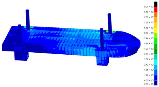
Figure 1.
Structural response of the WTIV under design-wave loading, MPa.
3. Optimized Structural Design of the Bracket Geometry
For the local structure at the toe of the bracket, parametric modeling technology was employed for optimization. Prior to developing the parametric modeling program, all parameters involved in the modeling process were clearly defined. For structural strength analysis, the modeling process included creating the geometric model, performing mesh generation, defining material properties, applying loads and boundary conditions, and finally conducting calculations using post-processing software. Subsequently, an optimization model was further established, incorporating design variables, constraint conditions, and the objective function.
3.1. Design Variables and Constraints
In the mathematical model, certain design parameters, such as the mechanical properties of the material, remain unchanged during the optimization process and are referred to as design constants. Another category of adjustable parameters, known as design variables, are modified iteratively to achieve the optimization objective. The number of design variables determines the dimensionality of the shape optimization design. As the dimensionality increases, the degrees of freedom also increase, potentially leading to a more favorable optimal solution; however, this also increases computational complexity and prolongs the calculation time [17]. Therefore, the number of design variables must balance multiple factors, and a smaller number of variables can simplify the optimization process while ensuring desirable results.
The free edge of the bracket was defined as either an elliptical arc or a circular arc. The transverse length, vertical height, and toe height of the bracket were adopted as the controlling parameters for the bracket geometry, while the bracket thickness was also included as a design variable for comprehensive consideration. When the transverse length equals the vertical height, the bracket becomes a circular-arc bracket.
In optimization design, each variable should be subject to certain restrictions, referred to as design constraints. These constraints are generally expressed as functional expressions of the design variables, known as constraint functions or constraint conditions. Constraint conditions can be categorized into two types: boundary constraints and state constraints [18]. Boundary constraints limit the range and type of values for the design variables, such as dimensional ranges and plate thickness. For the present vessel, due to limitations on the effective deck area, the horizontal arm length of the bracket is required to be within 500–600 mm, while the vertical arm length must be within 500–700 mm.
State constraints typically involve capacity and do not directly restrict the design variables themselves but are instead related to functions of the design variables. By limiting these functions, the design variables are indirectly constrained. For example, in structural optimization, requirements such as keeping the stress below the allowable stress or ensuring that a certain strength meets the relevant standards fall under state constraints. The constraints are therefore expressed as follows:
- (1)
- The toe height shall not exceed the thickness at the bracket toe and shall not be less than 15 mm.
- (2)
- When analyzed using a refined mesh model, the yielding capacity must satisfy the allowable stress requirement, with the criterion expressed as: .
3.2. Objective Function and Optimization Results
The stress concentration factor is a parameter that reflects the degree of local stress amplification. A higher value indicates that the stress concentration point is subjected to greater stress, which increases the likelihood of crack initiation under cyclic loading. Reducing the stress concentration factor can therefore enhance the fatigue strength performance of the structure. Consequently, minimizing the stress concentration factor in the target region was set as one of the optimization objectives.
The stress concentration factor is defined as:
where is the interpolated principal stress within the stress concentration region of the target structure, and is the nominal far-field stress.
In optimizing the bracket geometry, the objective function was formulated with the aim of enhancing structural safety while minimizing or avoiding any significant increase in the bracket’s weight. Considering that the weight of the bracket is relatively small compared with other primary structural components and that its main purpose is to reduce stress and improve the mechanical performance of the structure, the safety factor was assigned a higher weighting than the weight constraint.
A multi-objective optimization of the bracket geometry was performed using the simulated annealing algorithm. Although only four design variables were considered, this method was selected for its robust capability to escape local minima and effectively locate the global optimum. Simulated annealing is particularly well-suited for multimodal optimization problems, enabling stable convergence and comprehensive exploration of the design space even when the number of variables is limited. The optimization model expressed in Equation (4) and the optimization results presented in Table 2 and Table 3.
Table 2.
Variable and parameter values of the bracket before and after optimization.
Table 3.
Structural response of the bracket before and after optimization.
Where and are the stress concentration factors at the two bracket toes shown in Figure 2, respectively. As shown in Table 2 and Table 3, the dimensions of the bracket were significantly reduced after optimization, with the bracket mass decreasing by approximately 12%, the peak stress reduced by about 26%, and the stress concentration factor lowered by 2.58% and 17.77%, respectively. The results indicate that, despite the substantial reduction in bracket mass, all parameter indices of the bracket were maintained at or below their original levels, demonstrating that the optimized bracket improved material utilization efficiency and reduced economic cost. Furthermore, disregarding other strength considerations, the initial bracket design exhibited considerable redundancy in yield strength. Shape optimization effectively reduced this redundancy, decreased the weight, enhanced material utilization, and improved the overall performance of the bracket.
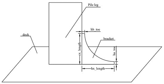
Figure 2.
Local structural stress response of the piled bracket.
4. Fatigue Testing of the Typical Joint
4.1. Fatigue Test Design
Since the E550 high-strength steel used in the critical structural components of this project has a yield strength exceeding the applicable range of material yield stress (≤400 MPa) for conventional S–N curves, it is necessary to conduct fatigue strength testing of the typical joint in the target structure to obtain a reasonable fatigue S–N curve and fatigue characteristics for the welded E550 steel. Fatigue testing on a full-thickness structural model can better reflect the fatigue performance of high-strength steel in critical structural joints; therefore, full-thickness structural fatigue tests were carried out in this study.
The fatigue test model design mainly followed the principles below:
- (1)
- Conduct a full-ship finite element analysis to determine the stress distribution induced by the primary loads acting on the hull, focusing on high-stress regions, and select the locations for model testing.
- (2)
- Based on the structural characteristics of fatigue-affected regions, and considering a feasible test setup, the fatigue strength test model for the typical joint was designed.
- (3)
- Define different loading levels, conduct fatigue strength tests on the typical joint under these levels, and obtain fatigue life values at various stress levels. On this basis, establish the S–N curve for the joint.
According to the above analysis, the fatigue test scheme for the joint was developed. In designing the test model, to ensure that the loading at the fatigue hotspot accurately reflects actual conditions, the plate thickness, material, geometry, welding configuration, and welding process at the hotspot and fatigue-affected regions were kept consistent with those of the real vessel, and the principal stress distribution at the hotspot was also matched to that of the actual ship. The test model was equivalently simplified under these constraints. The bracket and the upper plate adjacent to the bracket (corresponding to the deck in the actual vessel) were made of E550 steel, while the web and flange plates of the girder beneath the deck were made of EH36 steel. The model has the form of a “cantilever beam,” as shown in Figure 3.
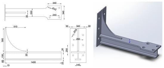
Figure 3.
Structural diagram of the typical joint specimen.
To ensure that the stress distribution in the specimen during testing is consistent with that of the actual vessel, a structural finite element analysis of the specimen was conducted. A rigid fixed constraint was applied to the left end plate of the specimen, and a concentrated load of 15.8 t was applied to the right end of the cantilever beam structure. The finite element calculation results are shown in Figure 4, where the high-stress regions are highlighted in red. As can be observed, significant stress concentration occurs at the bracket toe, and the stress distribution is generally consistent with that obtained from the full-ship structural strength analysis, indicating that the model is reasonable.
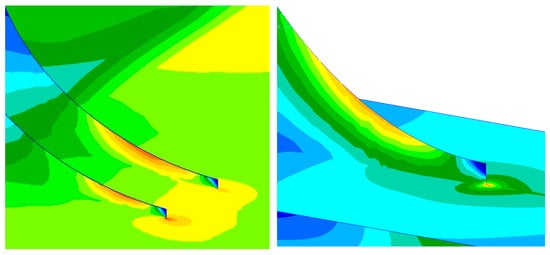
Figure 4.
Comparison of stress distribution between the full-ship model and the test model.
To verify the rationality of the fatigue specimen design for the typical joint, a comparative analysis of the stress distribution characteristics at the free edge and the toe hotspot of the bracket was conducted between the actual ship structure and the specimen, based on finite element analysis results. For the free-edge stress, dummy beam elements were created along the curved free edge of the bracket, and the axial stress distribution was obtained in their local coordinate system. For the toe stress, two rows of shell elements in the deck region perpendicular to the toe were selected, and the stresses at the centroid of each element were extracted. These were then interpolated pairwise to obtain the variation curve of the toe stress along the ship’s length.
To verify the rationality of the test design, both the stresses and the element distances of the actual ship and the specimen were nondimensionalized, and their stress distribution characteristics were compared. Taking the connection between the bracket and the pile-support frame as the origin of the coordinate axis, the distances of both structures were divided by the bracket width to obtain the nondimensional distance. Under this definition, the nondimensional distance at the bracket toe is 1, and the nondimensional distance corresponding to twice the bracket width, representing the far-field stress, is 2, as illustrated in Figure 5.
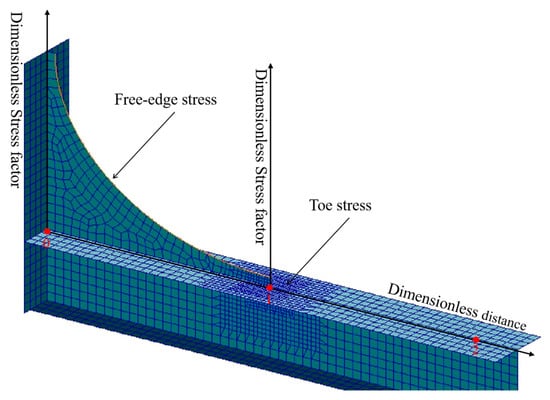
Figure 5.
Stress extraction at the bracket free edge and toe.
For the bracket free edge, the nondimensional stress coefficient was defined as the stress at a given location divided by the maximum stress along the free edge. For the bracket toe, the nondimensional stress coefficient was defined as the stress at a given location divided by the nominal far-field deck stress.
As shown in Figure 6, the stress distribution trends of both the free edge and the toe are generally consistent between the actual hull structure and the designed specimen, indicating that the specimen design is reasonably accurate.
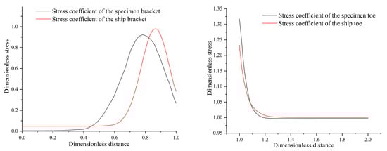
Figure 6.
Comparison of stress distribution between the bracket free edge and toe.
4.2. Fatigue Test
All specimens were fabricated in strict accordance with the qualified welding procedure, and non-destructive inspections were carried out to ensure their quality. Magnetic particle testing (MT) and ultrasonic testing (UT) were performed on all specimens, and the results confirmed that they met the inspection requirements, with no detectable surface or subsurface defects.
The fatigue specimens were tested at three stress levels, with two specimens at each level, resulting in a total of six specimens. Load-controlled testing was performed using an electro-servo fatigue testing machine, applying a sinusoidal load with a frequency of 2 Hz. The load ratio for the test was R = 0.1. The fatigue tests setup is shown in Figure 7.
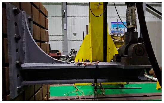
Figure 7.
Fatigue test of the typical joint.
Since the welded toe of the bracket is a high-risk location for structural fatigue failure, the toe stress was selected as the controlling parameter for fatigue assessment when establishing the S–N curve. According to the requirements of the CCS Rules [19], the toe stress should be calculated by linear interpolation of the principal stresses measured at positions t/2 and 3t/2 from the weld toe, as specified in Equation (5). Accordingly, during the fatigue test, three-axis strain gauges (Kyowa Electronic Instruments Co., Ltd., Tokyo, Japan) were installed at these two positions to obtain the principal stress data at each point.The schematic diagram of the stress measurement locations is shown in Figure 8.
where is the toe stress, and and are the principal stress at the positions located t/2 and 3t/2 away from the weld toe.
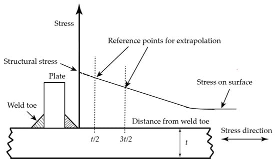
Figure 8.
The determination of the toe stress.
During the test, the strain data obtained from the three-axis strain gauges at the two measurement points were recorded in real time using a data acquisition system (DH5902, Donghua Testing Technology Co., Ltd., Jiangsu, China). Based on the plane stress assumption, the measured strain values in the three directions were substituted into the generalized Hooke’s law. Together with the material’s elastic modulus and Poisson’s ratio, the in-plane stress components at the corresponding location were calculated. Subsequently, the magnitude and orientation of the principal stresses were determined using the stress transformation equations, as described in Equation (6).
where is the strain in the 0° direction, is the strain in the 45° direction, and is the strain in the 90° direction.
When a visible crack appeared in the toe region, the specimen was deemed to have experienced fatigue failure. The test was then terminated, and the corresponding stress range S and number of load cycles N were recorded. The summarized results for the six specimens are presented in Table 4.
Table 4.
Test data of specimens under different stress levels.
In addition, detailed experimental data for all specimens under different loading conditions are provided in the Supplementary Materials (Tables S1–S10) for reference and reproducibility verification.
4.3. Fitting of the S–N Curve
In the logarithmic coordinate system, the S–N curve is expressed as
For each stress range obtained from the test, the calculated value of the logarithmic fatigue life can be determined using Equation (7) as follows:
According to the principle of univariate linear regression, the criterion for obtaining the best-fit straight line is to minimize the sum of the squared differences between the measured value and the calculated value [20]. Under this condition, m and lgA are obtained using the following formulas:
By substituting the fatigue test data listed in Table 4 into Equations (9) and (10), the S–N curve for the bracket toe weld of the typical joint can be obtained, with its expression given in the form of Equation (11).
For ease of comparison with the S–N curve specified in the standards, the S–N curve for the bracket toe of the typical joint was plotted in bilogarithmic form together with the D-curve from the standards in the same figure, as shown in Figure 9. It can be seen from the figure that the fatigue S–N curve of the E550 steel welded bracket toe lies above the D-curve specified in the standards. This indicates that, for the same stress range, E550 steel must undergo a greater number of load cycles before failure occurs, demonstrating that the fatigue strength of the E550 steel welded bracket toe is superior to the fatigue strength corresponding to the D-curve in the standards.
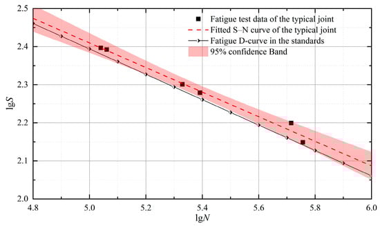
Figure 9.
S–N curve of the typical joint.
According to commonly used fatigue design standards, including DNV-RP-C203, and CCS [21,22], a high-cycle S–N slope of approximately 3 is typically adopted for welded steel joints. In this study, the slope of the S-N curve was found to be 3.1, which is in close agreement with the value of 3 specified in the standards. Additionally, the yield strength of the material specified in the standards is lower than that of E550 steel, which explains why the S-N curve for E550 steel appears slightly higher than the curve from the standards. This observation is consistent with the material properties and supports the reasonableness of the results.
The 95% confidence band for the experimental data is shown in Figure 9. This band represents the uncertainty range associated with the fitted S–N curve. As seen from the band’s width in the figure, its narrowness indicates the stability and reliability of the fit. Moreover, the alignment between the experimental data points and the fitted curve, along with the confidence band, suggests that the model accurately captures the fatigue behavior under the tested conditions.
5. Fatigue Analysis of the Bracket Toe in the Target Ship Structure
5.1. Linearization of Morison’s Equation
Under the standing condition of wind turbine installation, the legs of the self-elevating wind turbine installation vessel penetrate into the seabed, and sufficient foundation bearing capacity is established through preloading. The hull platform is then supported by the legs and elevated above the water surface, thereby achieving a stable operational posture.
At this stage, the environmental loads are dominated by wave actions, which primarily act on slender members such as the exposed legs, supporting trusses, and spudcans. For structural members whose diameters are small relative to the wavelength, the hydrodynamic force in the flow direction can be decomposed into inertia and drag components according to Morison’s concept. In engineering practice, the Morison equation is applied by segmental integration along the water depth to estimate the loads acting on the legs.
In the marine environment, wave loads exhibit stochastic characteristics, and engineering evaluations are generally conducted using frequency-domain methods within the framework of superposition and spectral analysis. However, the drag term in Morison’s equation is proportional to the square of the relative velocity, representing a nonlinear component.
When substituted into spectral analysis, this nonlinearity introduces frequency convolution in the frequency domain, making it difficult to directly solve the structural response and perform fatigue assessments using conventional spectral methods. To maintain the feasibility of frequency-domain analysis under random sea states and to establish a practical engineering approach, this drag term is linearized under conditions applicable to engineering practice.
This simplified method introduces errors, and we will briefly discuss the impact of linearization. The error tends to increase with lower significant wave height and observation height, often leading to an underestimation of fatigue damage, which negatively affects fatigue assessment. Additionally, the wave period also influences the error. In the sea area we are considering, where the significant wave height is relatively low, the impact of these errors is particularly important. At the lowest significant wave height and observation height, the fatigue damage error can reach 40%. As the observation height increases, the error decreases. However, the error at the lowest observation height does not represent the average total error, but rather the maximum error near the water surface. Therefore, under the worst-case scenario, the fatigue damage error will not exceed 40%. The drag term in Morison’s equation is expressed as follows [23]:
where is the density, is the drag coefficient, and is the diameter of the pile leg of the wind turbine installation vessel.
For an Airy wave in finite water depth, the velocity potential can be expressed as:
In the equation, is the angular frequency, is the first-order wave number, and is the water depth.
Then the fluid particle velocity can be expressed as:
By combining Equations (12) and (14), the drag term becomes:
In the equation, a is the wave amplitude. For the form in Equation (15), its Fourier series expansion can be written as:
where .
By retaining only the first term, the first-order linear expression of the drag is obtained as follows:
Through the above treatment, the drag term in Morison’s equation has been equivalently linearized under engineering application conditions, as shown in Equation (17). On this basis, the linearized drag term can be combined with the wave spectrum to establish the statistical distribution of wave loads under different wave heights and periods, thereby enabling the calculation of the equivalent wave drag acting on the pile legs. Furthermore, by applying this wave drag to the structural finite element model, the corresponding structural dynamic response can be obtained. Finally, based on spectral analysis theory, the fatigue damage of the structure under random sea states can be evaluated.
5.2. Fatigue Spectral Analysis Method
In ocean engineering, accurately simulating the irregularity of ocean waves is crucial for predicting the structural response of ships and offshore platforms. One of the most commonly used methods to describe the ocean surface in spectral fatigue analysis is through the wave spectrum, which approximately represents the energy distribution of waves at different frequencies [8]. The most commonly used wave spectrum is the two-parameter Pierson–Moskowitz (PM) spectrum, , which is expressed as:
where HS is a significant wave height, TZ is the zero-crossing period, and ω is the wave frequency.
In the analysis, the actual response frequency should be the encounter frequency ωe, which is related to the wave frequency ω, heading angle θ, and ship speed as follows:
Accordingly, the input wave spectrum should be converted into a wave spectrum , expressed in terms of the encounter frequency and related to the wave heading angle θ. This can be achieved by applying the energy conservation relationship for the differential elements of the corresponding wave frequency.
According to Equation (20), the wave spectrum expressed in terms of the encounter frequency can be obtained as:
Under the assumption that the ship structure is a linear system, the stress energy spectrum can be obtained from the following:
where is the stress transfer function.
Then, the nth order spectral moment of the response process for a given heading can be described as follows:
To obtain the number of stress cycles within a given time, the mean zero-crossing rate of the alternating stress process must be provided, which represents the average number of times the process crosses the zero mean with a positive slope per unit time [24]. Its expression is:
The cumulative fatigue damage from spectral analysis is obtained directly by combining the cumulative fatigue damage values from each short-term distribution, as calculated using Equation (25). Considering Nload loading conditions, the cumulative fatigue damage over the design service life is expressed as:
where D is the cumulative fatigue damage over the fatigue calculation return period; is the operation rate coefficient, selected according to the vessel’s actual operating conditions, and taken as 0.5 in this study; TL is the vessel’s design fatigue life, taken as 20 years in this study; A and m are the two parameters of the S–N curve; is the zeroth-order moment of the stress response spectrum for the loading condition under sea state and heading ; and are the occurrence probabilities of sea state and heading , respectively; and is the zero-crossing rate of the stress response under sea state and heading , calculated using Equation (24).
5.3. Fatigue Damage Analysis
This study primarily focuses on calculating and analyzing the fatigue damage at the hotspot of the bracket toe at the root of the pile-support frame. During fatigue calculations, the finite element mesh near the hotspot should be sufficiently refined to capture variations in the stress gradient.
In accordance with commonly used fatigue design standards, such as DNV-RP-C203 and CCS [21,22], the following meshing rules were applied when refining the finite element model around the fatigue hotspots in this study. The mesh size at the hotspot was limited to not exceed the local plate thickness t. The refined mesh region was extended in all directions from the hotspot by at least 10t. A smooth transition in mesh density was maintained between the refined and coarse mesh regions. In the refined mesh area, four-node quadrilateral elements were employed, and the use of triangular elements was avoided as much as possible. The results of the mesh refinement are shown in Figure 10.
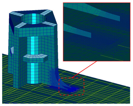
Figure 10.
Refined mesh diagram of the pile-support frame toe.
The significant wave height is a key factor affecting the strength of ship structures. Fatigue damage is not only related to the significant wave height Hs, but also to the zero-crossing period Tz, the probability of different sea states, and other factors. Therefore, fatigue damage is highly sensitive to scatter diagrams. Considering the ship operating area, wave scatter data from the coastal regions of China were selected for calculating the structural stress response transfer function [9]. The probability distribution of waves under different periods and wave heights is shown in Figure 11.
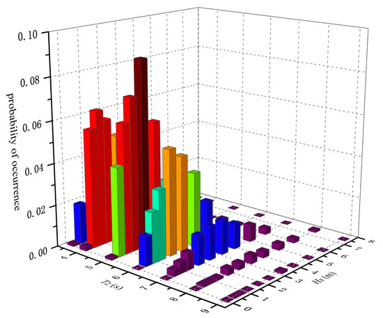
Figure 11.
Wave scatter probability diagram.
According to DNV-RP-C203 [21], the wave heading range for fatigue analysis should cover 0–360° with intervals not larger than 30°. In this study, 12 wave directions were selected at 30° intervals, with the occurrence probability of each direction set to 1/12. The calculated natural frequency range was 0.1 rad/s to 2.0 rad/s, with an interval of 0.1 rad/s, giving a total of 20 frequencies. For the standing condition, the hydrodynamic loads were directly calculated using the linear Morison equation described earlier. For the sailing condition, the hydrodynamic calculations were performed using the COMPASS-WALCS 2.0 wave load software developed by the China Classification Society. In this way, the pressure on each element of the ship’s wetted surface under unit wave amplitude could be obtained for different operating conditions.
In Patran 2019, the water pressure was applied, and the inertia release method was used to calculate the structural response. After obtaining the stress response distribution of the structure, the interpolation method described in Equation (5) and illustrated in Figure 8 was employed to derive the stress response at the hotspot. Consequently, the stress response transfer functions under different wave directions and frequencies were obtained, as shown in Figure 12.
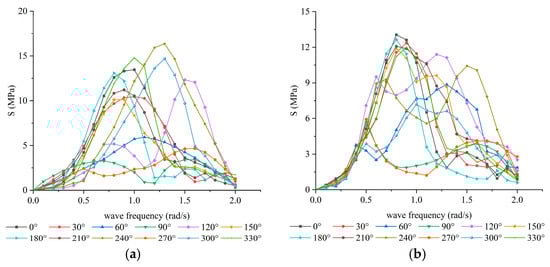
Figure 12.
Stress transfer function as follows: (a) Standing condition, (b) Sailing condition.
For the wind turbine installation vessel examined in this study, the design service life is 20 years, and the duration distributions of the sailing and standing conditions are shown in Table 5.
Table 5.
Operating condition schedule of the wind turbine installation vessel.
At this stage, by combining the stress response transfer function with the spectral fatigue analysis method, the total fatigue damage of the target vessel over 20 years can be calculated. The results are presented in Table 6.
Table 6.
Total fatigue damage over the 20-year design life.
A comparison of the fatigue damage data in Table 6 reveals that the damage under the standing condition is significantly higher than that under the sailing condition. This difference is primarily attributed to two factors: first, the standing condition lasts longer, leading to more pronounced cumulative effects; second, once the pile legs penetrate into the seabed and extend above the water, the bending moment acting on the pile-support frame increases, thereby causing stronger stress concentration.
This trend can also be verified by the stress responses in Figure 12: the maximum stress response under the standing condition is 32.8 MPa, whereas that under the sailing condition is 26.2 MPa. The difference between the two results in distinct damage distributions.
Over the design service life, the total damage of the pile-support frame of the target vessel is 0.60, which is below the allowable limit specified in the standards. In comparison, the damage of the pre-optimized structure was 1.08, exceeding the limit and not meeting the fatigue safety requirements.
After considering the error introduced by the linearization of Morison’s equation, the results still meet the design requirements. This indicates that the optimization design proposed in this study can effectively satisfy fatigue safety requirements and demonstrates both rationality and engineering applicability.
The distribution of fatigue damage across different wave headings varies significantly depending on the operating condition. Under the Standing condition, the most severe fatigue damage occurs at a wave heading of 240°, corresponding to oblique waves. Similarly, for the Sailing condition, the maximum fatigue damage is observed at a wave heading of 210°, also associated with oblique waves. This directional dependence highlights the importance of considering wave orientation in fatigue analysis. The specific values of the fatigue damage for each condition are presented in Table 7.
Table 7.
Fatigue damage under different wave headings for standing and sailing conditions.
The distribution of fatigue damage varies significantly across different sea states. Under the Standing condition, the most severe fatigue damage occurs in a sea state with a wave height of 3.25 m and a wave period of 6 s. Similarly, under the Sailing condition, the maximum fatigue damage is observed in a sea state with the same wave height of 3.25 m and wave period of 6 s. This indicates that the combination of these particular wave characteristics contributes most significantly to fatigue damage in both conditions. The specific values of fatigue damage under these sea states are presented in Figure 13, providing a clearer comparison of the damage distribution in different operational conditions.
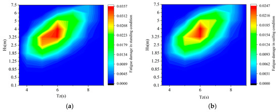
Figure 13.
Fatigue Damage Distribution: (a)Standing condition, (b)Sailing condition.
6. Conclusions
This study first employed a parametric modeling approach to optimize the geometry of the bracket at the root of the pile-support frame. Based on the local stress distribution similarity criterion, a fatigue test model for the bracket at the root of the pile-support frame was designed, and a fatigue test on the bracket’s local structure was carried out. The fatigue S–N curve of the E550 high-strength steel bracket toe was obtained, and, using this S–N curve, a fatigue strength evaluation of the bracket was performed. The following conclusions can be drawn:
- The parametric modeling approach can effectively achieve the shape optimization of the bracket structure. After optimization, the bracket changed from equal arm lengths to unequal arm lengths, with the horizontal arm being shorter than the vertical arm.
- To ensure that the model test accurately reflects the fatigue performance of the actual ship, the stress distribution at the hotspot of the fatigue model should match that of the actual ship. Using a full-thickness plate model can effectively simulate the stress distribution around the bracket of the pile-support frame in the actual ship.
- For the two high-stress regions—the bracket free edge and the bracket toe—the fatigue test results showed that fatigue cracks appeared only at the welded bracket toe, while no fatigue cracks were observed at the bracket free edge.
- The fatigue test produced the S–N curve for the E550 steel bracket toe, which exhibits a fatigue strength superior to that of the D-curve specified in the standards. The E550 steel bracket toe fatigue S–N curve obtained from the fatigue test can provide reference data for related fatigue design and analysis.
- Based on the spectral fatigue analysis, the total fatigue damage of the vessel over its 20-year design life meets the required safety standards. The maximum fatigue damage occurs at a wave heading of 240° under the standing condition and at 210° under the sailing condition, with both directions contributing most significantly to the overall fatigue response. Additionally, the most critical sea state for both conditions is characterized by a wave height of 3.25 m and a wave period of 6 s.
Supplementary Materials
The following supporting information can be downloaded at: https://www.mdpi.com/article/10.3390/jmse13112069/s1, Table S1: Calculation of stress range S for Specimen No. 1, Table S2: Calculation of stress range S for Specimen No. 2, Table S3: Calculation of stress range S at Load Level 1, Table S4: Calculation of stress range S for Specimen No. 3, Table S5: Calculation of stress range S for Specimen No. 4, Table S6: Calculation of stress range S at Load Level 2, Table S7: Calculation of stress range S for Specimen No. 5, Table S8: Calculation of stress range S for Specimen No. 6, Table S9: Calculation of stress range S at Load Level 3, Table S10: Summary of stress–life data of all load levels.
Author Contributions
Conceptualization, G.G. and G.F.; methodology, G.G. and G.F.; software, S.C.; validation, K.L. and S.C.; formal analysis, G.G.; investigation, K.L.; resources, G.F.; data curation, S.C.; writing—original draft preparation, G.G.; writing—review and editing, G.F.; visualization, S.C.; supervision, G.F.; project administration, G.F.; funding acquisition, G.F. All authors have read and agreed to the published version of the manuscript.
Funding
This research was supported by the National Key Research and Development Project (No. 2023YFA1609100).
Data Availability Statement
The original contributions presented in this study are included in the article/Supplementary Materials. Further inquiries can be directed to the corresponding author.
Conflicts of Interest
The authors declare no conflicts of interest.
References
- Tjaberings, J.; Fazi, S.; Ursavas, E. Evaluating operational strategies for the installation of offshore wind turbine substructures. Renew. Sustain. Energy Rev. 2022, 170, 112951. [Google Scholar] [CrossRef]
- Yang, Y.; Fu, J.; Shi, Z.; Ma, L.; Yu, J.; Fang, F.; Chen, S.; Lin, Z.; Li, C. Performance and fatigue analysis of an integrated floating wind-current energy system considering the aero-hydro-servo-elastic coupling effects. Renew. Energy 2023, 216, 119111. [Google Scholar] [CrossRef]
- Jin, J.Z.; Gao, Z. State-of-the-art and prospects of installation methods for offshore wind turbines. Ship Boat 2024, 35, 1–20. [Google Scholar] [CrossRef]
- Edwards, E.C.; Holcombe, A.; Brown, S.; Ransley, E.; Hann, M.; Greaves, D. Trends in floating offshore wind platforms: A review of early-stage devices. Renew. Sustain. Energy Rev. 2024, 193, 114271. [Google Scholar] [CrossRef]
- Jiang, Z. Installation of offshore wind turbines: A technical review. Renew. Sustain. Energy Rev. 2021, 139, 110576. [Google Scholar] [CrossRef]
- Gupta, S.; Shabakhty, N.; van Gelder, P. Fatigue damage in randomly vibrating jack-up platforms under non-Gaussian loads. Appl. Ocean Res. 2006, 28, 407–419. [Google Scholar] [CrossRef]
- Shabakhty, N. System failure probability of offshore jack-up platforms in the combination of fatigue and fracture. Eng. Fail. Anal. 2011, 18, 223–243. [Google Scholar] [CrossRef]
- Wang, Y. Spectral fatigue analysis of a ship structural detail—A practical case study. Int. J. Fatigue 2010, 32, 310–317. [Google Scholar] [CrossRef]
- Liu, Y.; Ren, H.; Feng, G.; Sun, S. Simplified calculation method for spectral fatigue analysis of hull structure. Ocean Eng. 2022, 243, 110204. [Google Scholar] [CrossRef]
- Leimeister, M.; Kolios, A. Reliability-based design optimization of a spar-type floating offshore wind turbine support structure. Reliab. Eng. Syst. Saf. 2021, 213, 107666. [Google Scholar] [CrossRef]
- d NSantos, F.; Noppe, N.; Weijtjens, W.; Devriendt, C. Data-driven farm-wide fatigue estimation on jacket-foundation OWTs for multiple SHM setups. Wind Energy Sci. 2022, 7, 299–321. [Google Scholar] [CrossRef]
- Park, J.S.; Yi, M.S. Review of structural strength in the event of a one-leg punch through for a wind turbine installation vessel. J. Mar. Sci. Eng. 2023, 11, 1153. [Google Scholar] [CrossRef]
- Huynh, V.V.; Nguyen, H.V.; Pham, T.N.; Do, Q.T. Local fatigue assessment of welded joints between leg and spudcan structures connection in jack-up wind turbine installation vessel. J. Ocean Eng. Mar. Energy 2025, 11, 987–1006. [Google Scholar] [CrossRef]
- Li, Z.; Mao, W.; Ringsberg, J.W.; Johnson, E.; Storhaug, G. A comparative study of fatigue assessments of container ship structures using various direct calculation approaches. Ocean Eng. 2014, 82, 65–74. [Google Scholar] [CrossRef]
- Kim, M.H.; Kang, S.W.; Kim, J.H.; Kim, K.S.; Kang, J.K.; Heo, J.H. An experimental study on the fatigue strength assessment of longi-web connections in ship structures using structural stress. Int. J. Fatigue 2010, 32, 318–329. [Google Scholar] [CrossRef]
- Kim, S.; Hauteclocque, G.; Bouscasse, B.; Lasbleis, M.; Ducrozet, G. Experimental analysis of extreme wave loads on a containership. Ocean Eng. 2024, 306, 118031. [Google Scholar] [CrossRef]
- Mei, L.; Wang, Q. Structural Optimization in Civil Engineering: A Literature Review. Buildings 2021, 11, 66. [Google Scholar] [CrossRef]
- Rigo, P. A module-oriented tool for optimum design of stiffened structures—Part I. Mar. Struct. 2001, 14, 611–629. [Google Scholar] [CrossRef]
- CCS. Guidelines for Fatigue Strength Assessment of Offshore Engineering Structures; China Classification Society: Beijing, China, 2022. [Google Scholar]
- Zhen, C.; Feng, G.; Wang, T.; Yu, P. Numerical and Experimental Study on Trimaran Cross-Deck Structure’s Fatigue Characteristics Based on the Spectral Fatigue Method. J. Mar. Sci. Eng. 2019, 7, 62. [Google Scholar] [CrossRef]
- DNV-RP-C203; Fatigue Design of Offshore Steel Structures. DNV: Høvik, Norway, 2024.
- CCS. Guidelines for Fatigue Strength of Hull Structures; China Classification Society: Beijing, China, 2022. [Google Scholar]
- Kim, H.-J.; Lee, K.; Jang, B.-S. A linearization coefficient for Morison force considering the intermittent effect due to free surface fluctuation. Ocean Eng. 2018, 159, 139–149. [Google Scholar] [CrossRef]
- Zhang, M.; Yu, H.C.; Feng, G.Q.; Ren, H.L. Investigation on effects of springing and whipping on fatigue damages of ultra-large container ships in irregular seas. J. Mar. Sci. Technol. 2021, 26, 432–458. [Google Scholar] [CrossRef]


Disclaimer/Publisher’s Note: The statements, opinions and data contained in all publications are solely those of the individual author(s) and contributor(s) and not of MDPI and/or the editor(s). MDPI and/or the editor(s) disclaim responsibility for any injury to people or property resulting from any ideas, methods, instructions or products referred to in the content. |
© 2025 by the authors. Licensee MDPI, Basel, Switzerland. This article is an open access article distributed under the terms and conditions of the Creative Commons Attribution (CC BY) license (https://creativecommons.org/licenses/by/4.0/).