1. Introduction
During the navigation of a fully skirted hovercraft, the stability of the cushion pressure is crucial for safe operation. However, due to the unique and complex structure of the skirts, modeling and controlling the cushion system poses significant challenges [
1,
2]. With the rapid advancement of artificial intelligence and the continuous improvement in computational capabilities, researchers are no longer limited to spending extensive time and effort on modeling and controlling such complex systems solely through traditional methods. Instead, deep learning-based modeling [
3,
4,
5] and reinforcement learning-based control [
6,
7,
8] have emerged as increasingly popular research directions. Therefore, exploring how to apply deep reinforcement learning to model and control the complex cushion system of a fully skirted hovercraft constitutes a key focus and challenge of this study.
Numerous studies have been conducted on cushion pressure control for fully skirted hovercrafts [
2,
9,
10]. An adaptive fuzzy sliding-mode control method to regulate the cushion pressure of hovercrafts by controlling the lift fans was proposed in [
9]. An adaptive neural network to adjust the parameters of the PID controller was introduced in [
2], thereby enhancing the stability control of the cushion pressure. Similarly, reference [
10] utilized the DDPG reinforcement learning algorithm to tune the parameters of a PID controller for autonomous cushion height control. However, the aforementioned methods all simplify the complex hovercraft cushion system into a second-order system for controller design, thereby not only neglecting the inherent characteristics of the hovercraft cushion dynamics but also yielding control strategies with limited practical relevance for real-world cushion pressure regulation.
Traditional Reinforcement Learning (RL) relies on interaction with the real environment to make action decisions, and it has achieved preliminary applications in certain low-cost domains such as small unmanned aerial vehicles (UAVs) [
11,
12] and unmanned ground vehicles (UGVs) [
13,
14]. A multi-agent reinforcement learning method based on both extrinsic and intrinsic rewards was proposed in [
12] to collaboratively control the behavior of UAVs for target encircling tasks. To address the challenge of capturing escaping targets with UGVs, Su et al. [
13] decomposed the reward function into individual and cooperative components, optimizing both global and local incentives. By enhancing cooperation among the pursuing UGVs, this approach significantly improves the capture success rate. However, in applications involving large-scale equipment or specific domains where the cost of trial-and-error is prohibitively high, its practical implementation remains challenging [
15]. In contrast, offline reinforcement learning eliminates the need for real-time interaction with the environment. Instead, it leverages pre-collected datasets—generated in real or simulated environments—to learn policies and make decisions, thereby mitigating safety risks and reducing training costs associated with online interaction. As a result, offline reinforcement learning has emerged as a growing research direction and has attracted broad attention from researchers and experts across disciplines [
16,
17].
Deep Learning (DL) models are deep neural network architectures characterized by multiple nonlinear mapping layers, which are capable of extracting features from input signals and uncovering underlying patterns [
18]. The Long Short-Term Memory (LSTM) network, an enhanced variant of Recurrent Neural Networks (RNNs), has been widely adopted in numerous time series studies, including applications such as speech recognition [
19], multimedia audio and video analysis [
20], and road traffic flow prediction [
21]. In hovercraft systems, the relationship between fan speed and chamber pressure is highly nonlinear, involving complex physical processes such as fluid dynamics and aerodynamics [
2]. However, in the field of hovercraft lift system research, particularly in the use of LSTM for predicting cushion pressure, no relevant studies have been reported to date.
Based on the above analysis, this paper addresses the challenges of modeling the lift system, cushion pressure instability, and control delays in hovercraft by proposing a deep reinforcement learning-based predictive control method for cushion pressure. The main contributions of this work are summarized as follows:
- (1)
An LSTM-based predictor with a temporal sliding window is proposed for hovercraft cushion pressure forecasting, effectively capturing the dynamic coupling between fan speed and chamber pressure while explicitly incorporating inherent control lag.
- (2)
A novel adaptive behavior cloning mechanism is integrated into the TD3-BC framework, which dynamically balances the RL objective and historical policy constraints via an auto-adjusted weight, thereby mitigating distribution shift and policy degradation in offline settings.
- (3)
A fully data-driven control architecture is established by combining the LSTM predictor with the adaptive TD3-BC algorithm, abbreviated as LSTM-TD-BC, enabling accurate cushion pressure tracking, improved motion stability, and extended lift fan operational life through reduced rotational speed fluctuations.
The remainder of this paper is structured as follows:
Section 2 introduces the mathematical model of the hovercraft lift system and related preliminary knowledge.
Section 3 details the proposed LSTM-TD3-BC-based cushion pressure prediction and control framework.
Section 4 presents simulation results and comparative evaluations. Finally,
Section 5 concludes the paper and suggests future research directions.
3. Prediction and Control of Air Chamber Pressure in Air Cushion Vehicle Based on LSTM-TD3-BC
To enable real-time prediction and active control of the chamber pressure in a fully cushioned hovercraft, this section employs an improved LSTM network to forecast the chamber pressure. This approach is designed to capture the complex spatiotemporal dynamics inherent in the hovercraft’s cushion system, thereby establishing a model foundation for subsequent reinforcement learning-based control of the cushion pressure. Building on the LSTM-based prediction model for the lift system, offline policy optimization is performed using the TD3-BC reinforcement learning algorithm. This enhances both the stability and robustness of the system while maintaining accurate control over the cushion lift pressure.
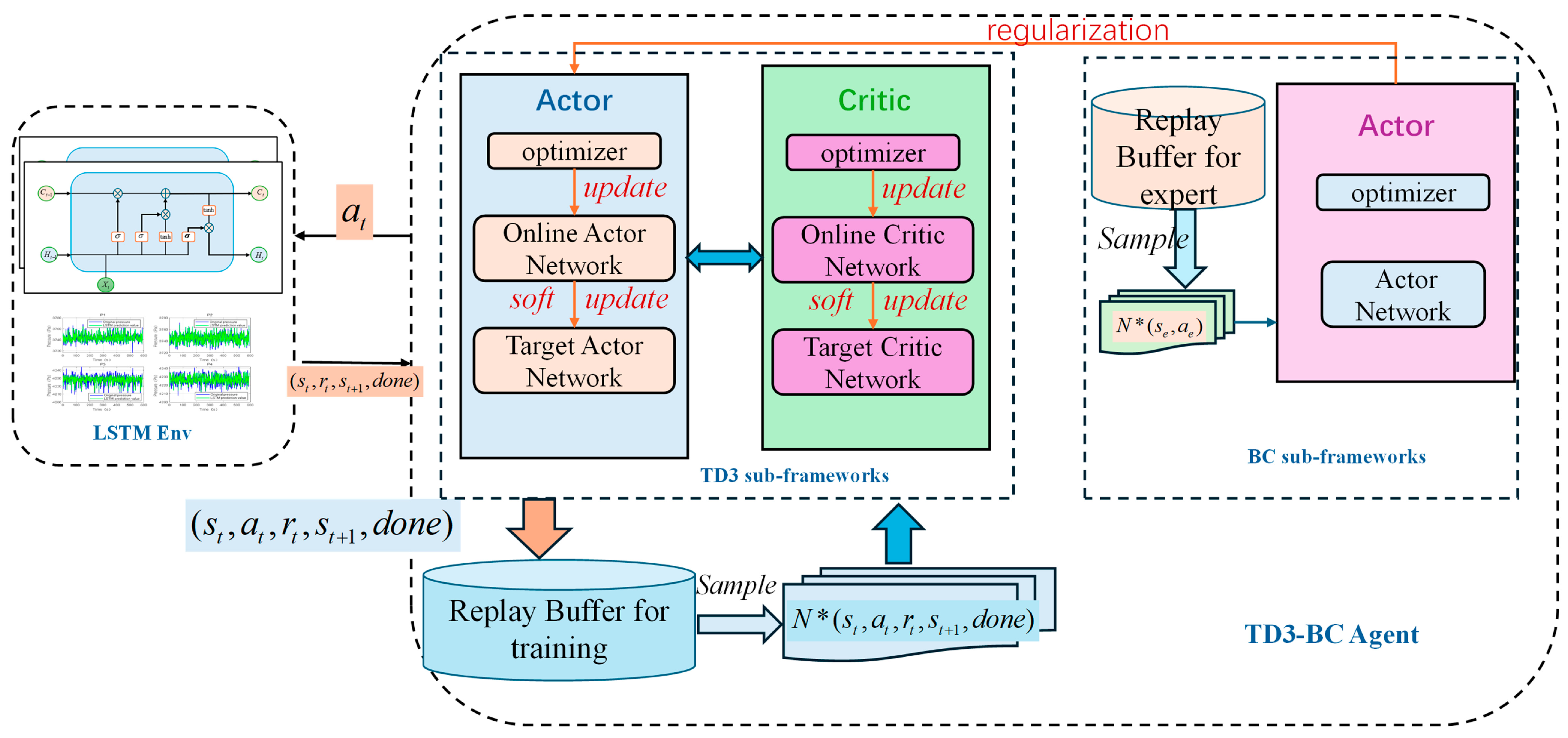
A schematic diagram of the hovercraft chamber pressure prediction and control framework based on the LSTM-TD3-BC algorithm is presented in
Figure 3. The LSTM Prediction Model serves as the environment for the RL agent, forecasting chamber pressures based on the history of system states. The TD3 Algorithm serves as the primary RL controller, generating control actions (fan speed increments) based on the current state and its Q-value estimates. The Behavior Cloning (BC) Framework regularizes the TD3 policy by constraining it towards actions demonstrated in the historical dataset, using an adaptive weight to mitigate distribution shift.
3.1. LSTM Deep Learning Model
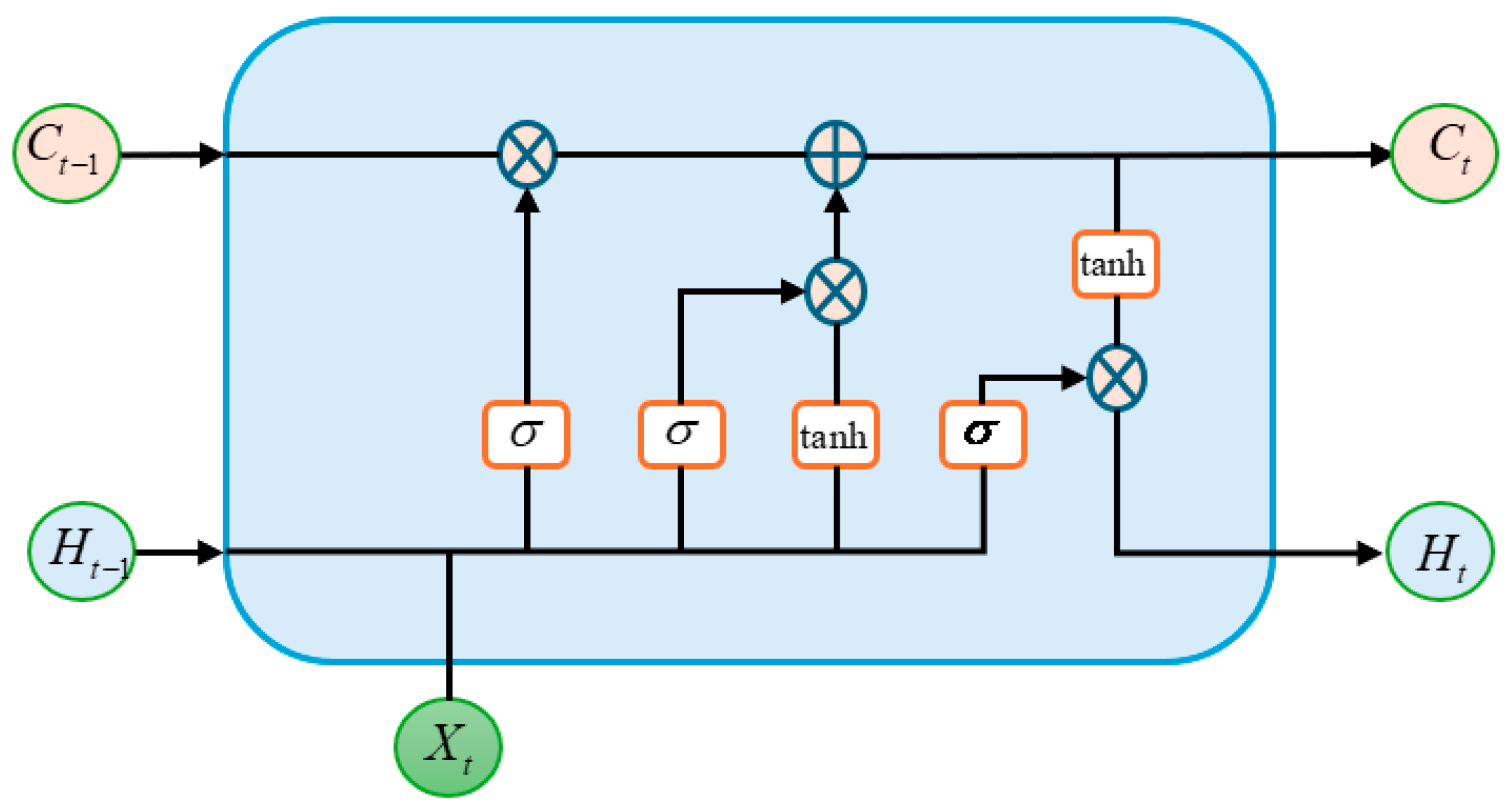
LSTM network is an improved model of recurrent neural network (RNN). LSTM learns long-term correlated information by introducing gating mechanism to control the forgetting and flow of information, thereby alleviating the gradient explosion and vanishing problems of RNN during training. Therefore, LSTM is an ideal choice for processing time-series data [
24]. The overall structure of LSTM is shown in
Figure 4. The LSTM network mainly consists of four modules, namely input gate, forget gate, memory unit, and output gate, and continuously updates the states of the four modules to process the sequence data in each time step.
In
Figure 4,
is the input data information at time
,
is the hidden state information,
is the memory unit state, and
is the hyperbolic tangent activation function.
is a
activation function, which compresses the input value between 0 and 1 to ensure whether information is retained or forgotten.
The forget gate controls the retention and forgetting of information in the memory unit. Based on the current state and the previous hidden state, obtain an information value representing the degree of forgetting. The higher the value, the greater the probability of the corresponding information being forgotten in memory unit
. This mechanism allows LSTM to selectively retain long-term dependent available information, discard low value data, and effectively process complex sequence data. The calculation formula is expressed as follows:
where
is the output of the forget gate,
is the weight matrix between the current input and the forget gate,
is the weight matrix between the historical output and the forget gate, and
is the bias term of the forget gate.
The input gate serves to update the memory cell state by determining whether new information should be retained. It processes the previous hidden state and the current input through a sigmoid activation function, producing output values between 0 and 1, where 0 signifies insignificance and 1 indicates importance. Meanwhile, the same inputs are processed by a
function to generate candidate memory cell states within the range of −1 to 1. The output of the input gate is expressed as follows:
where
denotes the output of the input gate,
represents the weight matrix between the input gate and the input,
is the weight matrix connecting the previous hidden state to the input gate, and
denotes the bias term of the input gate.
The candidate cell state represents the extent to which the new input at the current time step can influence the memory cell state. It is computed as follows:
where
is the candidate cell state,
denotes the weight matrix between the input and the candidate state,
represents the weight matrix associated with the previous hidden state, and
is the bias term.
The memory cell serves as the core component of the entire LSTM network. It is capable of not only regulating the flow and update of information but also storing and transmitting data. After incorporating the information from the forget gate and the input gate, the memory cell state can be updated as follows:
The output gate regulates the flow of information passed to the next time step. It determines which parts of the cell state should be output Via a sigmoid activation function. The output of the gate is expressed as follows:
where
denotes the weight matrix between the input and the output gate,
represents the weight matrix connecting the previous hidden state to the output gate, and
is the bias term of the output gate. Subsequently, the hidden state
is obtained by multiplying the output gate with the cell state processed through a
activation function, as follows:
3.2. TD3-BC Reinforcement Learning Algorithm
To mitigate the high interaction cost and safety risks associated with online reinforcement learning, researchers have introduced offline reinforcement learning [
25]. Offline reinforcement learning trains a policy
using a pre-collected dataset. The agent executes an action
in state
according to the policy, and the expected cumulative return after following the policy
is given by the following:
It represents the expected cumulative discounted return when the agent starts from state , executes action , and thereafter follows policy . The expectation accounts for the inherent randomness in both the policy and the environment’s state transitions.
Equation (24) is updated Via the Bellman equation as follows:
This provides a recursive decomposition of the value. It states that the Q-value for a state–action pair can be broken down into the immediate reward and the discounted expected value of the next state , where is the state resulting from taking action in state . This recursion is fundamental to most RL algorithms, as it enables iterative estimation and improvement of the Q-function.
Equation (25) can be solved by minimizing the mean squared Bellman error, which is defined as follows:
This serves as the primary loss function for training the Critic network in value-based RL methods like TD3. By minimizing this loss, the parameters of the Q-network are adjusted so that its estimates become increasingly consistent with the Bellman Equation (25).
Essentially, the objective of offline reinforcement learning is to learn a policy that outperforms the behavior policy, thereby achieving improved performance upon deployment in real-world interactions. However, due to the issue of distribution shift, most offline RL algorithms tend to adopt conservative strategies, which often limits their ability to capture the full complexity of the policy when relying solely on behavioral cloning. Therefore, striking an effective balance between policy improvement and mitigating distribution shift constitutes a central challenge in the field of offline reinforcement learning.
TD3-BC is an offline reinforcement learning algorithm that integrates the advantages of both TD3 and BC [
26]. The TD3 component employs an Actor–Critic architecture along with a replay buffer of collected experiences. It updates the policy based on the value of the Q-function, prioritizing state–action pairs with high estimated returns regardless of the current policy behavior. This flexibility enables the algorithm to leverage large, sparse rewards effectively, thereby improving the success rate. Through advanced policy exploration, it derives an optimized policy, denoted as
. The BC component consists of an expert replay buffer and an Actor network, which learns from expert demonstrations to facilitate knowledge transfer.
TD3-BC incorporates a BC regularization term to ensure that the policy optimizes the Q-function while remaining close to the actions observed in the historical dataset. This prevents the algorithm from taking overly risky actions in regions with insufficient data coverage. Consequently, the policy optimization objective of TD3-BC is to maximize the following policy objective function:
where
denotes the dataset used for policy training, and
is the behavior regularization coefficient that controls the degree of conservatism by constraining the learned policy to remain close to the behavior policy. By default,
refers to the
norm (Euclidean norm), which has the same meaning when used in subsequent formulas.
3.3. Design of LSTM-TD3-BC-Based Algorithm for Cushion Pressure Prediction and Control
An LSTM network is employed to model the dynamic relationship between fan speeds and chamber pressures. The input to the model is a 6-dimensional state vector over a historical time window of length T, which consists of four chamber pressure values and two fan speed values, denoted as . The output is the predicted four chamber pressure values at the subsequent time step, denoted as .
To enhance the robustness of the LSTM prediction model, the Huber loss function is employed as follows:
where
is a positive constant.
The training process of the LSTM prediction model follows systematic data processing and deep learning optimization methodology, with key steps summarized in Algorithm 1. The procedure begins with standardized preprocessing of the raw time-series data from the air cushion vehicle lift system. The mean and standard deviation of each channel are computed to normalize the dataset into a zero-mean, unit-variance form.
Subsequently, input-output sample pairs are constructed using a temporal window slicing technique to predict the cushion pressure at the next time step. The model architecture employs a two-layer LSTM encoder, with a dropout layer (rate = 0.2) applied after the second LSTM layer to prevent overfitting. The Huber loss function is utilized to combine the advantages of both Mean Absolute Error (MAE) and Mean Square Error (MSE) loss functions, thereby enhancing the model’s robustness to outliers. The Adam optimizer is adopted with a learning rate
, and momentum coefficients
and
. The hyperparameters in Algorithm 1 were chosen based on established practices in deep learning for time-series problems and limited empirical tuning on our validation set. For instance, the time window size T = 20 was selected to balance the need to capture the system’s short-term dynamics with computational efficiency.
| Algorithm 1 Training Procedure for LSTM-Based Cushion Pressure Prediction Model |
| Input: | |
| | Time window size T = 20
|
| Output: | Trained LSTM prediction model |
| 1 | data preprocessing: |
| 2 | Calculate the mean and standard deviation of each channel |
| 3 |
|
| 4 | Split training and testing sets |
| 5 | Initialize LSTM model M: |
| 6 | Input layer: (T,6) Time window, feature dimension |
| 7 | LSTM1: Unit 128 |
| 8 | Dropout layer: 0.2 |
| 9 | LSTM2: Unit 128 |
| 10 | Fully connected layer, with dimensions of 4 |
| 11 | |
| 12 | for epoch to E do: |
| 13 | ) do: |
| 14 | forward propagation |
| 15 | Loss calculation |
| 16 | backpropagation |
| 17 | , parameters update |
| 18 | end for |
| 19 | |
| 20 |
|
| 21 | , Save LSTM model |
| 22 | end for |
| 24 | Return LSTM pressure prediction model
|
In the pressure control system of the hovercraft lift system, this paper adopts the TD3-BC algorithm as the core reinforcement learning framework. By integrating the TD3 with BC regularization, the algorithm effectively addresses the issues of extrapolation error and policy degradation in conventional offline reinforcement learning. To dynamically balance the strength of policy optimization and historical behavior imitation, and to ensure an effective trade-off between exploring novel actions and maintaining behavioral stability, this paper introduces an adaptive BC regularization method to update the objective function of the Actor network. Therefore, Equation (27) can be rewritten as follows:
where
is BC regularization strength, and
is the adaptive weighting coefficient defined as follows:
where
is a sufficiently small constant to prevent division by zero.
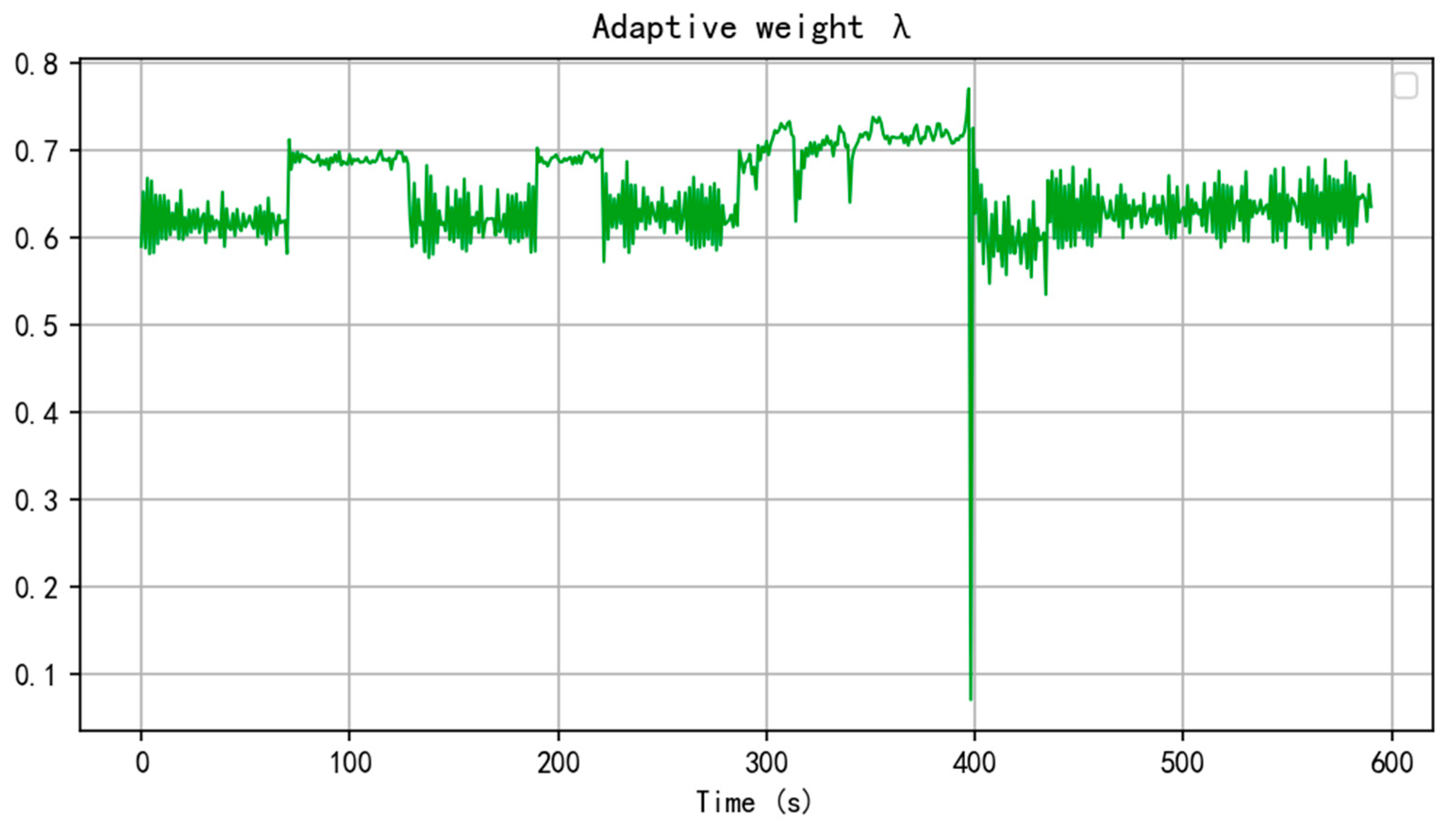
Remark 1. The primary role of the adaptive weighting coefficient is to dynamically balance the relative importance between the reinforcement learning objective and the behavior cloning constraint. When the policy performs poorly, indicated by unreliable and low Q-value estimates, increases to strengthen the influence of behavioral regularization. This encourages the policy to imitate expert behaviors from the historical dataset, thereby mitigating the risk of risky actions. Conversely, when the policy performs well, decreases to relax the behavior cloning constraint, allowing greater exploration for potentially superior strategies beyond historical behaviors.
The Critic network employs a twin Q-network architecture and is trained by minimizing the temporal difference (TD) error, which is derived from the Bellman equation:
where
. The target networks are updated via a soft update mechanism to ensure training stability, thereby guaranteeing control precision in hovercraft lift pressure control task and further enhancing system robustness. The pseudo-code of the TD3-BC-based cushion pressure control algorithm is presented in Algorithm 2:
| Algorithm 2 TD3-BC-Based Control for Hovercraft Cushion Pressure |
| Input: | |
| | LSTM prediction model M
|
| Output: | |
| 1 | Initialization: |
| 2 | Experience buffer zone Sampling from D |
| 3 |
|
| 4 |
|
| 5 | |
| 6 | for count in maximum iterations do: |
| 7 | , Batch sampling |
| 8 | , Target action calculation |
| 9 | , Target Q-value calculation |
| 10 | Update Critic Network: |
| 11 |
|
| 12 |
|
| 13 | then: |
| 14 | Adaptive BC weight update: |
| 15 |
|
| 16 |
|
| 17 | Actor loss for behavior cloning: |
| 18 |
|
| 19 | , Update actor |
| 20 | Soft update target network: |
| 21 |
|
| 22 |
|
| 23 |
|
| 24 | end if |
| 25 | end for |
| 26 | |
4. Experimental Results and Discussion
To evaluate the effectiveness of the proposed algorithm, this study utilizes a fully skirted hovercraft simulation platform to generate a cushion dataset during navigation for training the LSTM prediction model. The process is further integrated with the offline reinforcement learning algorithm TD3-BC to make reinforcement learning-based control decisions for cushion pressure regulation. The experiments were conducted in the following environment: hardware setup includes an Intel Core i7-13700KF CPU and an NVIDIA RTX 4060Ti GPU; software environment consists of Python 3.9, PyTorch 1.12.1, and CUDA 11.6; the simulation platform employs PyCharm 2022 for algorithm development and Visual Studio 2022 for hovercraft simulator integration.
The experiments utilized a simulator closely mimicking a real-world hovercraft to generate the dataset, which consists of 101,922 samples. Each sample includes a 7-dimensional feature vector: . All features, except time, were normalized using min-max scaling. Input sequences were constructed by applying a sliding window method with a history of 20-time steps, and the pressure values at the next time step were used as the output. The dataset was split into training and validation sets for the LSTM model in an 8:2 ratio. Subsequently, an adaptive TD3-BC algorithm was employed, integrating offline data and the LSTM prediction model, to achieve stable cushion pressure control through reinforcement learning-based decision-making.
This study adopts a simulation-based, data-driven experimental design, which is structured into three consecutive phases: (1) data collection, (2) predictive model training, and (3) offline reinforcement learning control. The specific details are as follows:
4.1. Simulation Study on Cushion Lifting Characteristics
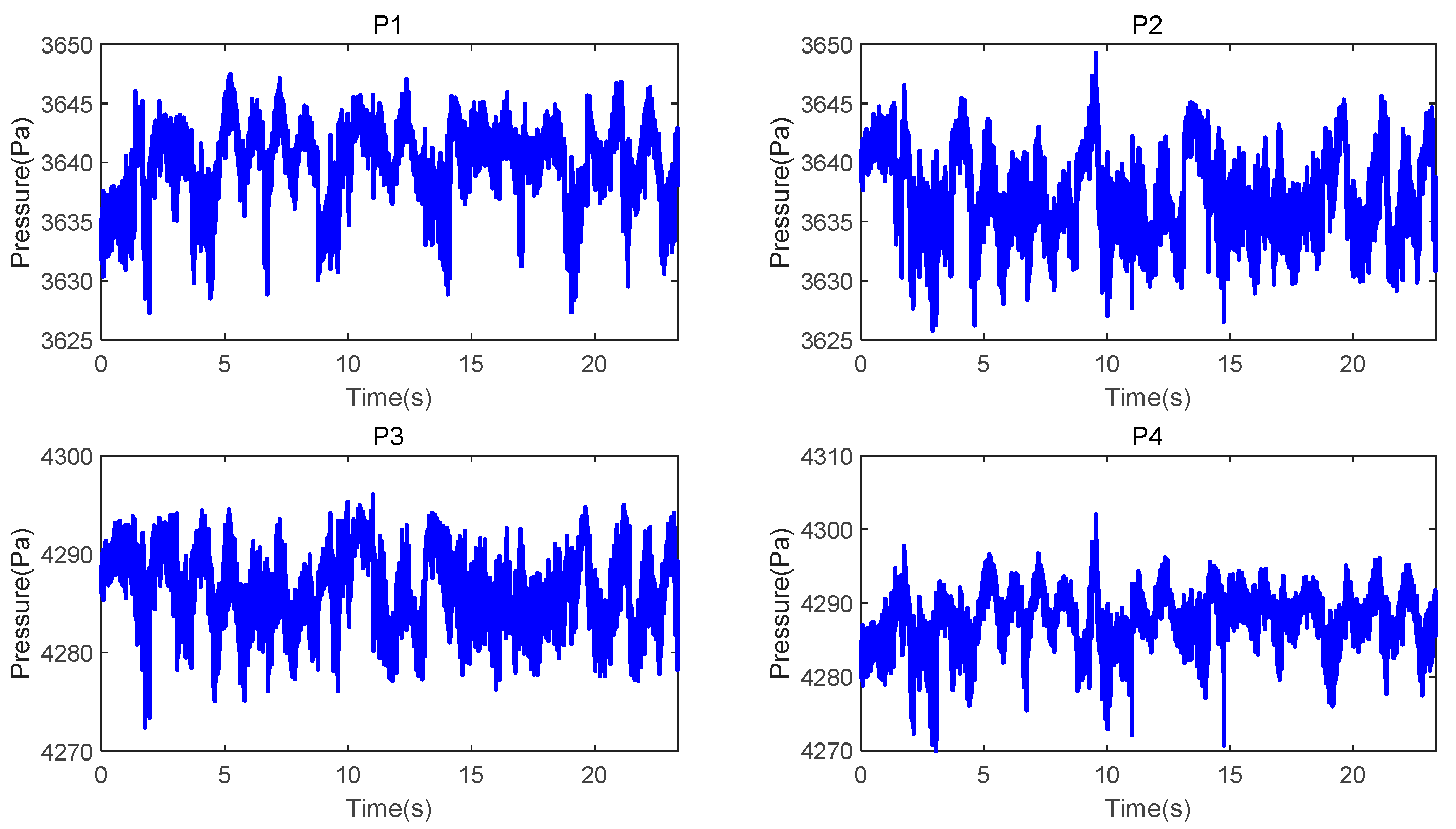
The cushion stability of a fully skirted hovercraft is fundamental to its safe navigation. After developing a mathematical model of the lift system, simulation was conducted to acquire pressure variation data of each air chamber under the influence of lift fan speeds and external environmental disturbances. The initial speed of the hovercraft was set to 25 knots, while the rotational speeds of the port and starboard lift fans were fixed at 2020 rpm. Partial simulation results illustrating the pressure changes in the air chambers of the cushion system are shown in
Figure 5 and
Figure 6.
As can be observed from
Figure 5 and
Figure 6, under constant lift fan speeds, the hovercraft exhibits significant pressure fluctuations and vibrations due to wave-induced disturbances and skirt air leakage. These effects result in considerable vertical oscillations during navigation, which not only impair crew operational safety but also compromise the hovercraft’s overall seakeeping performance.
4.2. LSTM Air Cushion Pressure Prediction
To validate the effectiveness of the proposed LSTM-based cushion pressure prediction model, its parameter configuration is provided in
Table 1. Using historical system states from the past 20 time steps and trained over 120 epochs on offline data, the model accurately predicts the pressure values of the four air chambers at the next time step.
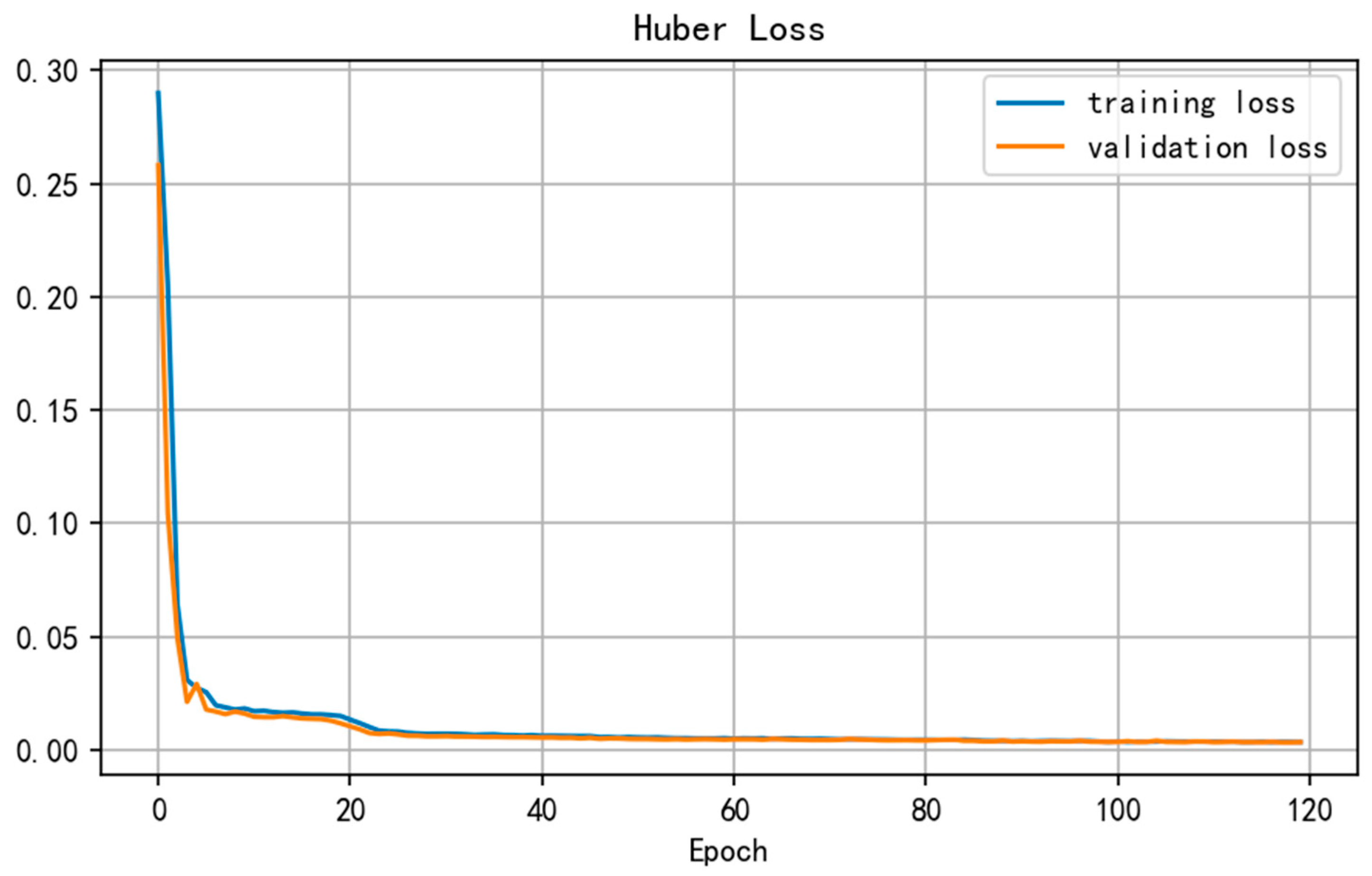
The training process of the prediction model is illustrated in
Figure 7. This study employs the Huber loss function, which combines the smooth convergence properties of MSE with the robustness of MAE against outliers. As can be observed, both the training loss and validation loss decrease synchronously as the number of iterations increases, converging after approximately 20 epochs without exhibiting overfitting. The stable convergence of the training process lays a foundation for obtaining a high-precision prediction model.
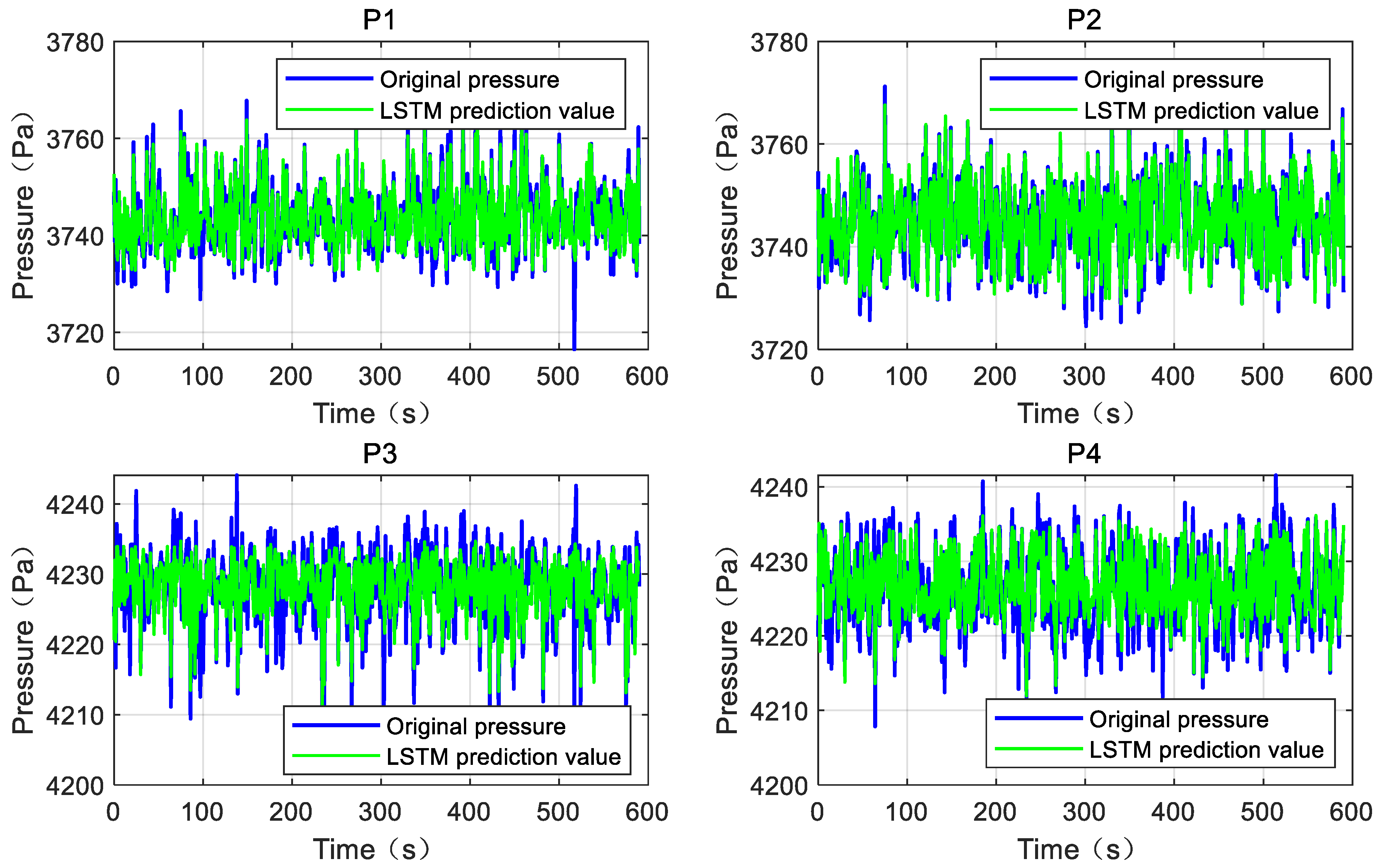
The pressure prediction results are shown in
Figure 8. To evaluate the prediction accuracy of the LSTM algorithm for the pressure in each air chamber, the mean absolute error (MAE), root mean square error (RMSE), and coefficient of determination (R
2) were adopted as evaluation metrics, as summarized in
Table 2. The proposed LSTM prediction model demonstrated outstanding performance on the test set: it achieved an average MAE of 2.2497 Pa and an average RMSE of 3.0337 Pa across the four air chambers, with a mean R
2 value of 0.7624. These results confirm the high prediction accuracy of the proposed method and establish a reliable foundation for subsequent offline reinforcement learning.
4.3. TD3-BC Reinforcement Learning Decision Control
To evaluate the performance of the TD3-BC algorithm in hovercraft cushion pressure control, this study compares the control effectiveness of the LSTM-based prediction model integrated with both the adaptively weighted TD3-BC and the conventional TD3 algorithm. We repeated the training process of the core adaptive TD3-BC algorithm multiple times with different random seeds, while keeping the dataset and LSTM prediction model fixed. All algorithms were executed under the same testing environment, and the parameter settings of the adaptive TD3-BC reinforcement learning approach are provided in
Table 3.
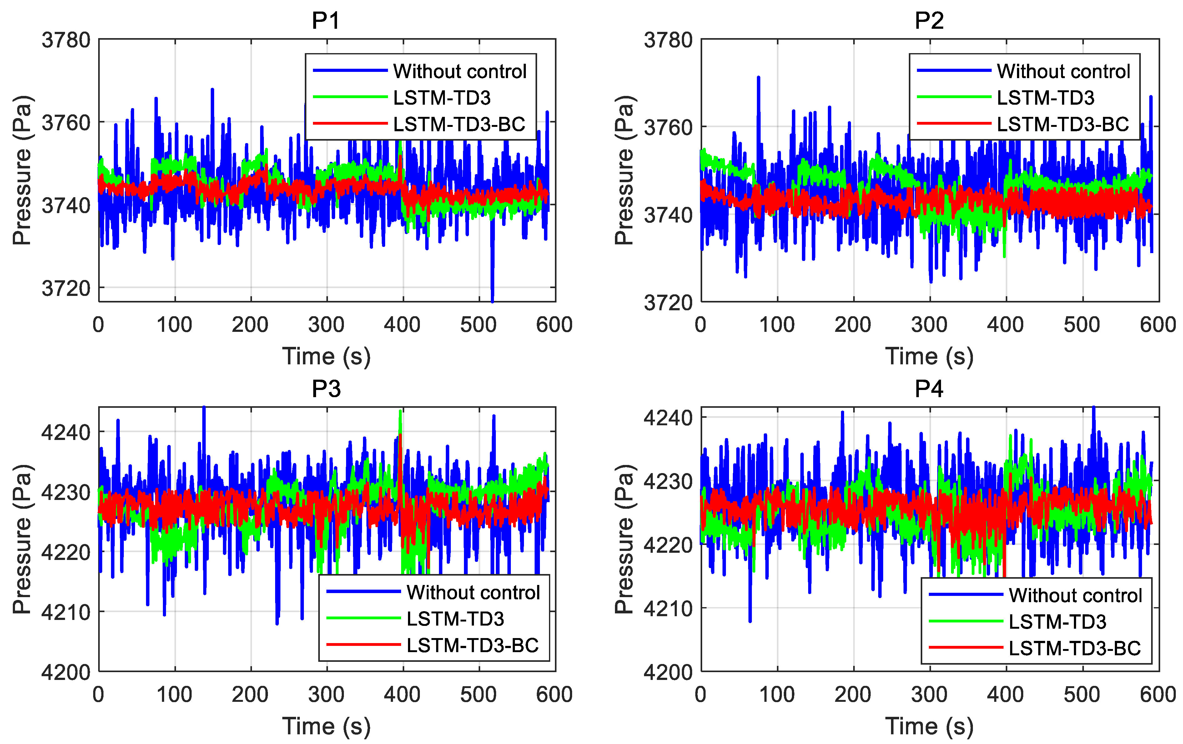
As shown in
Figure 9, compared to the uncontrolled cushion pressure and the LSTM-TD3 control algorithm, the proposed adaptively weighted LSTM-TD3-BC reinforcement learning algorithm effectively maintains the chamber pressure within the desired range with smoother adjustments.
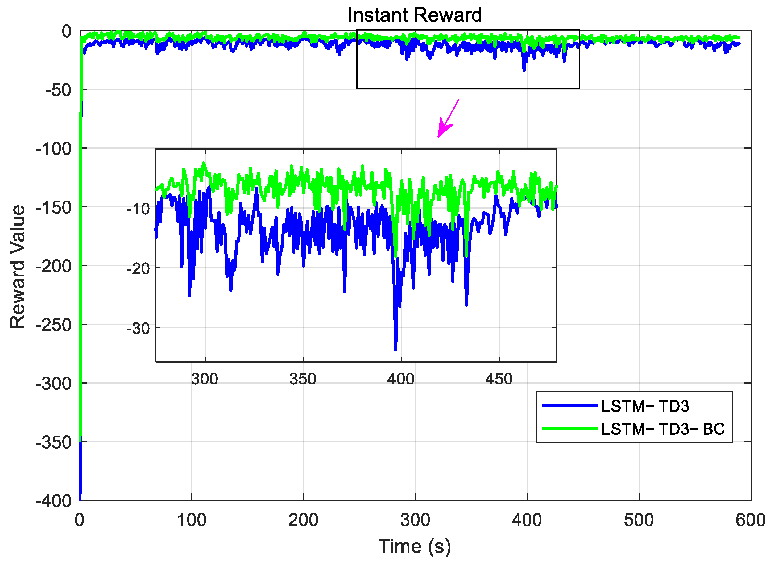
Figure 10 illustrates a comparison of lift fan speeds under different control algorithms. In contrast to the LSTM-TD3 method, the proposed adaptive LSTM-TD3-BC results in smaller fluctuations in fan speed, which not only stabilizes cushion pressure but also contributes to prolonged fan service life. The instantaneous reward curves are depicted in
Figure 11. Although both methods achieve stable chamber pressure, the adaptive LSTM-TD3-BC algorithm demonstrates more consistent learning performance, owing to the effective adjustment of adaptive weights, as further supported by
Figure 12.
In summary, the proposed adaptive LSTM-TD3-BC reinforcement learning-based predictive control method for hovercraft cushion pressure enables accurate prediction of chamber pressure and facilitates stable control decisions for cushion pressure regulation by leveraging historical experiential data and a reliable prediction model. Stable and autonomous control of cushion pressure is essential for the navigation of hovercrafts. Therefore, effective and smooth cushion pressure control lays a critical foundation for surface navigation control tasks. While the overall data collection was a single instance, the policy optimization and evaluation demonstrate stable and repeatable performance under random initialization, and that future work will involve testing across a wider variety of sea states and operational conditions.
5. Conclusions and Future Work
This paper proposed a deep reinforcement learning-based predictive control scheme for cushion pressure in fully skirted hovercraft, aiming to address the challenges of modeling complexity, pressure instability, and control delays in the lift system. Firstly, an LSTM network with a fixed-time window was employed to accurately predict chamber pressure, effectively capturing the dynamic coupling between fan speed and chamber pressure. Secondly, a novel adaptive behavior cloning mechanism was embedded into the TD3-BC framework, which dynamically balances the reinforcement learning objective and historical policy constraints through an auto-adjusted weighting coefficient, thereby effectively mitigating distribution shift and policy degradation in the offline RL setting. By integrating the LSTM prediction model with the adaptive TD3-BC offline reinforcement learning algorithm, stable cushion pressure control was achieved. Finally, simulations demonstrated that the proposed method not only improves the accuracy and robustness of chamber pressure prediction but also achieves smooth pressure control while reducing fluctuations in lift fan speed, thus extending the service life of the equipment. Future research will focus on refining the proposed method and implementing the algorithm in real-world cushion pressure control applications for fully skirted hovercraft.
While this study demonstrates the effectiveness of the proposed method, some limitations remain. Validation was conducted solely via simulation, creating a sim-to-real gap, and control performance depends heavily on the quality of the offline dataset. Future work will focus on implementing the algorithm on a real hovercraft platform through hardware-in-the-loop testing. We will also investigate adaptive data collection strategies, extend the framework to more extreme sea conditions, and incorporate additional practical constraints such as actuator saturation and safety guarantees.
