Article

Optimizing Informer with Whale Optimization Algorithm for Enhanced Ship Trajectory Prediction

Navigation College, Dalian Maritime University, Dalian 116026, China
*
Author to whom correspondence should be addressed.
J. Mar. Sci. Eng. 2025, 13(10), 1999; https://doi.org/10.3390/jmse13101999
Submission received: 15 September 2025 / Revised: 15 October 2025 / Accepted: 16 October 2025 / Published: 17 October 2025
(This article belongs to the Special Issue Ship Manoeuvring and Control)

Abstract

The rapid expansion of global shipping has led to continuously increasing vessel traffic density, making high-accuracy ship trajectory prediction particularly critical for navigational safety and traffic management optimization in complex waters such as ports and narrow channels. However, existing methods still face challenges in medium-to-long-term prediction and nonlinear trajectory modeling, including insufficient accuracy and low computational efficiency. To address these issues, this paper proposes an enhanced Informer model (WOA-Informer) based on the Whale Optimization Algorithm (WOA). The model leverages Informer to capture long-term temporal dependencies and incorporates WOA for automated hyperparameter tuning, thereby improving prediction accuracy and robustness. Experimental results demonstrate that the WOA-Informer model achieves outstanding performance across three distinct trajectory patterns, with an average reduction of 23.1% in Root Mean Square Error (RMSE) and 27.8% in Haversine distance (HAV) compared to baseline models. The model also exhibits stronger robustness and stability in multi-step predictions while maintaining a favorable balance in computational efficiency. These results substantiate the effectiveness of metaheuristic optimization for strengthening deep learning architectures and present a computationally efficient, high-accuracy framework for vessel trajectory prediction.

1. Introduction

With the rapid expansion of the global shipping industry, coupled with advances in ship intelligence and the trend toward larger vessels, maritime traffic density has been steadily increasing. This is particularly evident in complex waters such as ports and narrow channels, where high vessel density and diverse ship types elevate the risk of collisions, compromising not only navigation efficiency but also leading to property damage and even casualties [1]. The Automatic Identification System (AIS) serves as a critical technology for enhancing navigational safety. AIS data encompasses extensive dynamic and static information about vessels, along with objective maritime traffic regulations, making it a valuable big data resource [2]. Leveraging the vast amount of ship data provided by AIS to accurately predict future trajectories enables the timely identification of collision risks, thereby enhancing navigation safety and optimizing maritime traffic management.
Research on ship trajectory prediction has garnered significant attention from scholars worldwide. Current methods for predicting the trajectory of ships can basically be divided into several types of prediction method based on basic principles. The first one is statistical methods. The second group is machine learning methods. The third group is deep learning methods. Statistical methods generally formulating a kinematics equation according to a history of track data and predicting using the current condition of the ship. Wang et al. [3] established a dynamic model that contained geometric information of an object, and considered all the external factors affecting the dynamic behavior of an object, such as wind, water current, ship form, and stochastic motion characteristics, and formulated the mathematical model. The authors. Qiao et al. [4] proposed a Kalman filter-based prediction method to realize real-time trajectory prediction, updating the calculation of weighting factors for the state value of ships at successive time to predict the ships positions for next time [5] introduced an eXogenous Kalman Filter (XKF) algorithm which predicted ship movement based on real time port AIS data for ship motion visualization. But these ways depend on understanding beforehand to obtain the kinematics equations and because the ships paths are not straight predicting those movements well is hard to do.
Machine learning approaches on ship trajectory prediction mainly build models through historical vessel track patterns. Representative algorithms such as Artificial Neural Network (ANN) [6,7,8,9], Back Propagation Neural Network (BPNN) [10], Support Vector Machines (SVM) [11], etc., are often used. Liu et al. [12] also proposed SVR model, based on adaptive chaos differential evolution (ACDE) algorithm, it can effectively solve the SVR model prediction issues and the overall prediction accuracy, it can better solve the real-time issue Similarly, Zhang et al. [13] presented an improved K-nearest neighbor method, used to determine the future location of target ship by carrying out a weighted computation on every nearby vessel as well as their distance from the target at that particular point of time. Machine Learning approaches although providing more accurate predictions, they also face some problems because they are computationally expensive and do not have good generalization ability.
As deep learning continues to develop, driven by data ship trajectory prediction is becoming more and more common due to its robustness and generalizability [14]. Major architectures in this area make liberal use of Recurrent Neural Network (RNN) and its relatives, such as Long Short-Term Memory (LSTM) [15] and Gated Recurrent Unit (GRU) networks [16]. For instance, Qian et al. [17] used a Genetic Algorithm (GA) to optimize the hyperparameters of an LSTM prediction architecture. Another strategy, output optimization of the model: This approach refines the initial outputs of the neural network using a secondary optimization model to improve prediction realism and accuracy. Li et al. [18] introduced an improved Bidirectional LSTM (Bi-LSTM) model and applied the Radam and Lookahead Then on the experimental results, they found from their experiments that their improved model can have a good generalization of the problem, and they can have a better prediction. In a different approach Zhao et al. [19] utilized graphical attention network (GAT) which can better acquire the spatiotemporal characters and the hybrid GAT-LSTM having high robustness was proposed. Similar, Ju [20] also used Convolutional Neural Network (CNN) for the feature extraction process and replaced LSTM with GRU without reducing the prediction accuracy but the increased efficiency. Dong et al. [21] combined the Mish activation function with the CNN output to have better smooth nonlinear mapping and combined it with temporal attention, focusing on amplifying the important ones to achieve an optimized CNN-MTABiGRU. In terms of the application of GRU in time series forecasting, Jia et al. [22] introduced a method called Kalman-GRU, which uses GRU combined with a recursive Kalman filter for time series prediction. This utilizes the Kalman filter’s recursive estimation to cope with the problems caused by time and changing dynamics, as well as multimodality. Finally, Lin et al. [23] adopted Temporal Convolutional Network (TCN) on the trajectory prediction, proposing the improved Tiered-TCN (TTCN). They made a model called hybrid TTCN-Attention-GRU using it with Attention and a GRU network, taking the best parts of all its pieces to achieve really accurate answers.
While RNN-based models perform well for short-term trajectory prediction, their architecture makes it difficult to capture medium-to-long-term dependencies effectively. A significant breakthrough came in 2017 with Google’s introduction of the Transformer model [24]. A type of Encoder–Decoder Structure which can capture medium to long-term dependencies, it was a huge success for natural language processing (NLP) [25]. And this led to the transformer being applied to the task of trajectory prediction, at which time many scholars have utilized and further developed the transformer architecture which is much better than the traditional RNN approach. For example, Xu et al. [26] used a transformer as an enhancement to a Kalman Filter, where they used the transformer to utilize its great feature extraction and parallel computing power while the Kalman filter would use the Kalman filter to do dynamic real-time updates of the predictions in real time, which helps with the long-term dependencies for RNN. Xue et al. [27] added a GRU layer in the transformer and improved position embedding which leads to G-Trans. And this sort of collaboration between GRU and transformer is exceptionally advantageous pertaining to long-term prediction accuracy: similarly, Wang et al. [28] came up with a model which brings together Social Variational Autoencoder (Social-VAE) as well as Transformer and can capture the spatiotemporal dependencies that arise when lots of ships are interacting with each other. They found that their study showed that the model increased the prediction accuracy in the short-term and the medium to long term. Liu et al. [29] pioneered the application of Large Language Models (LLMs) to ship trajectory prediction. By leveraging prompt engineering and fine-tuning based on Low-Rank Adaptation (LoRA), their approach achieves cost-effective, high-precision forecasting, offering an efficient and novel solution for the field.
To overcome the well-documented limitations of the Transformer model, namely its quadratic time complexity and substantial memory footprint, the Informer model was introduced as an effective successor [30]. This architecture introduces a ProbSparse self-attention mechanism that effectively alleviates the computational burden of standard self-attention while maintaining modeling capacity. In the domain of ship trajectory prediction, Xiong et al. [31] demonstrated the Informer’s superiority over the Transformer, reporting enhanced performance and efficiency for medium-to-long-term forecasts. Their comprehensive experiments across varying input-output configurations further confirmed its state-of-the-art capabilities in multi-step trajectory prediction. To address the Informer’s occasional shortcomings in capturing local dependencies, Chen et al. [32] proposed the C-Informer, which integrates a Causal Convolutional Network (CCN) module to heighten sensitivity to adjacent temporal features, thereby tailoring the model more effectively for ship trajectory prediction.
The Informer model proves particularly adept at distilling salient features from AIS data, consistently delivering robust and accurate predictions for medium-to-long-term and multi-step ship trajectory forecasting. However, practical deployment requires adaptable prediction across varying time horizons, complicated by the inherent heterogeneity of vessel movement patterns. Consequently, realizing the model’s full potential requires meticulous, application-specific hyperparameter tuning. Manual tuning, however, is often subjective and inefficient, frequently converging to suboptimal local minima and thus failing to unlock the model’s peak performance [33]. Therefore, imperative to adopt advanced optimization algorithms to automate and enhance the hyperparameter selection process for the Informer model, a central motivation for the present study.
The Whale Optimization Algorithm (WOA), a meta-heuristic proposed by Mirjalili et al. in 2016 [34], has demonstrated unique capabilities in addressing complex optimization problems that are nonlinear, high-dimensional, non-differentiable, and multi-objective in nature [35]. In recent years, WOA has found widespread application in neural network optimization. For instance, Jia et al. [36] designed an Attention-BiLSTM network for single-step ship trajectory prediction. To address the challenge of hyperparameter selection, they integrated WOA to optimize the network’s parameters, with results indicating that the optimized model exhibited high applicability and stability. Similarly, Xie et al. [37] developed a CNN-BiGRU model for ship traffic flow prediction and utilized WOA to optimize its hyperparameters. Their results demonstrated a high consistency between predicted and actual values, with the error curve exhibiting only minor fluctuations. Han et al. [38] applied the Whale Optimization Algorithm (WOA) to optimize ship routing in complex marine environments, conducting comparative analyses with both Grey Wolf Optimizer (GWO) and Particle Swarm Optimization (PSO) algorithms. Their findings demonstrate that WOA achieves superior performance while exhibiting a notably stronger capability to escape local optima.
In summary, this paper presents a novel ship trajectory prediction method that integrates the WOA with the Informer model. The proposed approach leverages the Informer’s strengths in medium-to-long-term and multi-step forecasting, while employing WOA to fine-tune its built-in hyperparameters. This synergy enhances the model’s adaptability to specific prediction tasks, thereby maximizing the architecture’s potential. The main contributions of this paper are summarized as follows: (1) An end-to-end high-precision ship trajectory prediction framework is constructed. The framework comprises three core modules: AIS data preprocessing, trajectory pattern partitioning, and the WOA-Informer prediction model. It achieves a complete workflow from raw AIS data—pattern identification—adaptive deep prediction, forming a unified and scalable architecture for intelligent ship trajectory forecasting. (2) WOA is introduced into the hyperparameter tuning process of the Informer model, establishing a coupled framework between the optimization algorithm and the deep learning model. (3) A balance between prediction accuracy and computational efficiency is achieved. By combining KD-Tree acceleration, sparse attention mechanisms, and WOA-based optimization, the proposed model attains high accuracy with improved computational efficiency.
The remainder of this paper is structured as follows: Section 2 outlines the research methodology, including trajectory data preprocessing, clustering techniques, and the principles of the models employed. Section 3 evaluates the proposed framework through experimental validation and discussion. Section 4 concludes the study by summarizing the key findings and contributions, addressing the research limitations, and suggesting promising directions for future work.

2. Methodology

2.1. Overall Framework

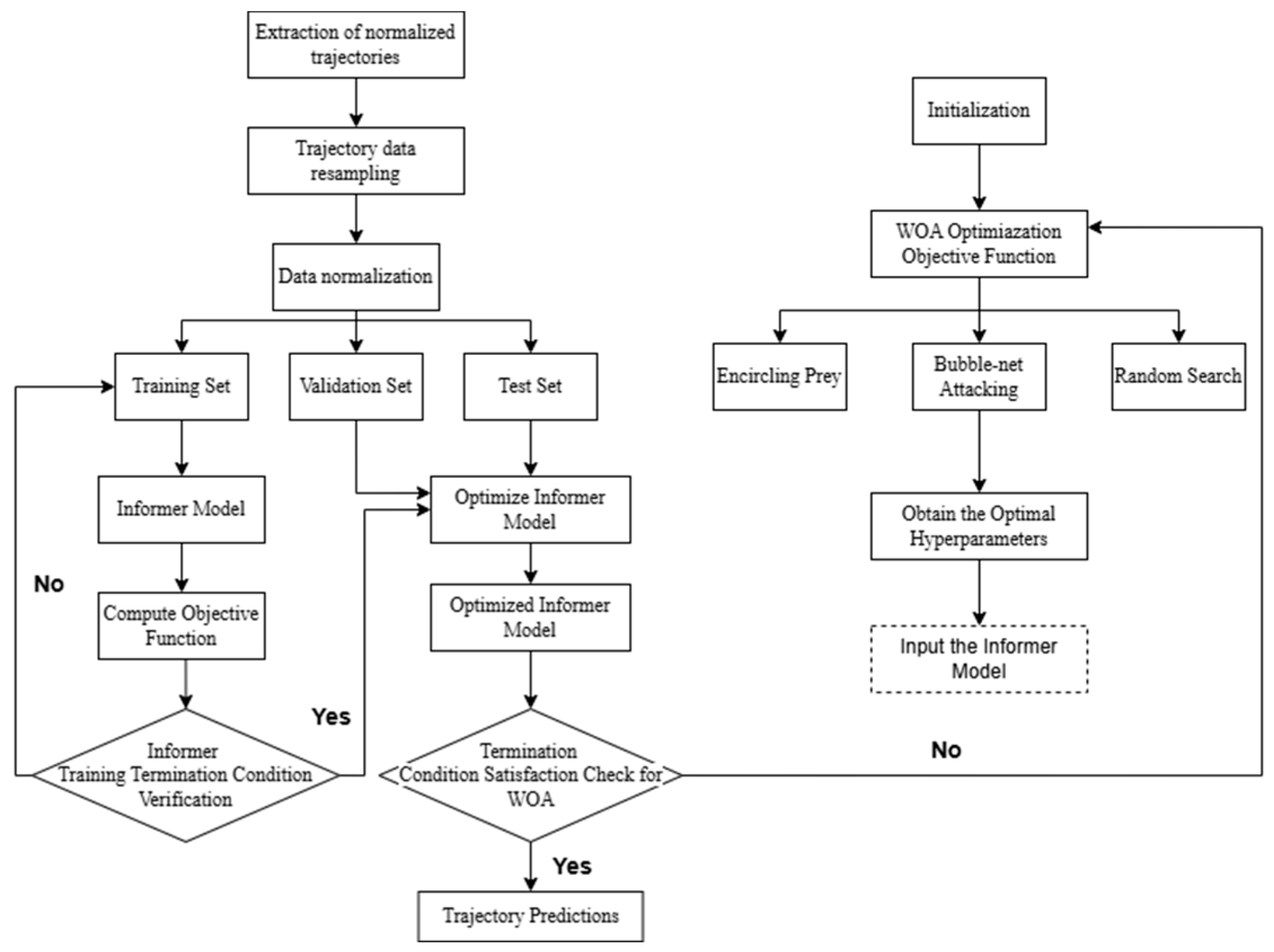
This study aims to develop an integrated ship trajectory prediction framework that combines the Whale Optimization Algorithm (WOA) with the Informer model, enhancing its adaptability to diverse trajectory patterns. To accomplish this objective, the research comprises three main components: (1) Data preprocessing: Raw AIS data undergoes extraction and cleaning to eliminate outliers and interpolate missing trajectory points, thereby enhancing overall data quality. (2) Trajectory clustering: Preprocessed trajectories are clustered using the DBSCAN algorithm, with Hausdorff distance calculations accelerated through KD-Tree spatial indexing and pruning strategies, significantly improving clustering efficiency. (3) WOA-Informer trajectory prediction: The process begins with extracting and resampling normalized trajectories from clustering results to obtain equidistant data. Subsequent normalization prepares the data for model training. Finally, the processed data is fed into the Informer model for prediction while WOA optimizes its architectural parameters. This approach enables automatic parameter adjustment tailored to specific trajectory patterns while minimizing training error, thereby reducing subjectivity in manual parameter selection and decreasing model construction time, ultimately enhancing both the accuracy and efficiency of trajectory predictions. The subsequent subsections provide detailed descriptions of the models and methodologies employed. The overall framework is illustrated in Figure 1, while Figure 2 depicts the WOA optimization process. The WOA-Informer optimization loop is presented in Algorithm 1.
Algorithm 1. WOA-Informer Optimization Loop
Input: AIS trajectory data D
Output: Optimized Informer model
1: Normalize and split D into Train, Val, and Test sets
2: Initialize WOA population {P_i}, i = 1…N
3: for each iteration t = 1…T do
4:   for each P_i do
5:     Train Informer with P_i; evaluate fitness E_i on Val set
6:    end for
7:    Update whales via encircling, bubble-net, and random search
8:    if termination condition met then break
9: end for
10: Train Informer with best P_best on Train + Val sets
11: Test optimized model and output trajectory predictions

2.2. AIS Data Preprocessing

High-quality Automatic Identification System (AIS) data is essential for reliable ship trajectory clustering and prediction. However, raw AIS datasets often contain substantial noise arising from signal interference, improper equipment usage, or human operational errors. Consequently, comprehensive data preprocessing is indispensable. This section summarizes prevalent quality issues in AIS data and outlines corresponding processing methodologies.
(1)
Outlier date removal: Three primary types of outliers are addressed: incorrect values, duplicates, and drift values. Incorrect values correspond to parameters such as longitude, latitude, speed, and course that fall outside plausible ranges (e.g., longitude beyond [−180°, +180°] or latitude beyond [−90°, +90°]). Duplicates are identical AIS records appearing in consecutive time periods. Drift values denote sudden, large deviations occurring over short durations within otherwise continuous trajectories, contradicting typical ship motion patterns. Such outliers adversely affect subsequent analysis and must therefore be removed.
(2)
Trajectory pruning via thresholds: Empirical observations indicate that trajectory segments with an insufficient number of AIS points lack the requisite information to characterize ship navigation patterns adequately, thereby impairing subsequent analysis. Consequently, segments containing fewer than 200 points are discarded.
(3)
Missing data imputation: Signal interruptions in AISs can result in missing data over certain time intervals. Common imputation techniques include mean interpolation, Lagrange interpolation, and spline interpolation. Among these, cubic spline interpolation offers high precision and has been extensively validated for AIS data imputation [39]. This study therefore employs cubic spline interpolation for missing data reconstruction. The cubic spline interpolation formula is given by Equation (1), where S i ( x ) denotes the spline function, x denotes the node, and a i , b i , c i , d i denote the 4n unknown coefficients.
S i x = a i + b i x + c i x 2 + d i x 3

2.3. Trajectory Clustering

2.3.1. Density-Based Spatial Clustering of Applications with Noise Algorithm

DBSCAN is a density-based clustering algorithm capable of grouping data points in high-density regions into clusters, identifying arbitrarily shaped clusters even in the presence of noise points, and demonstrating inherent robustness to noise [40]. DBSCAN offers distinct advantages for trajectory clustering applications: it requires no a priori specification of the number of clusters and can effectively discover trajectories with arbitrary shapes.
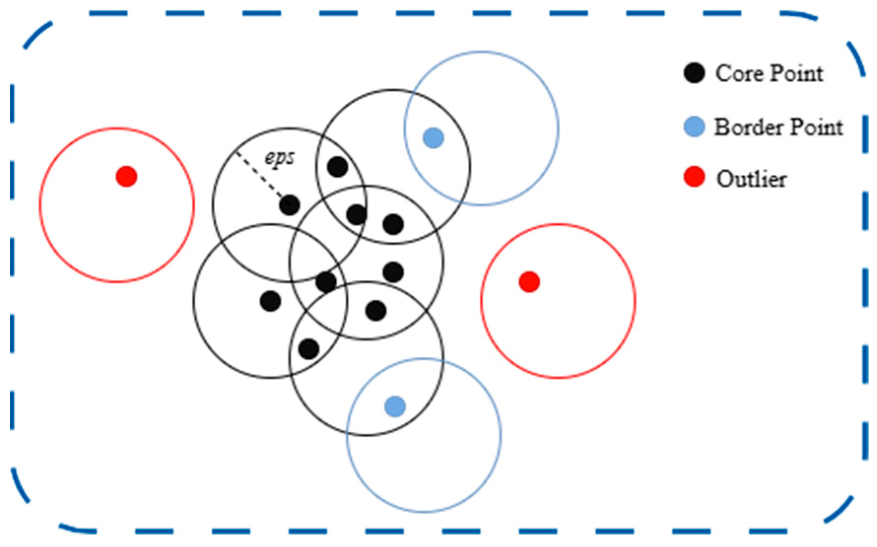
The algorithm operates with two key parameters: the neighborhood radius ( ε ) and the minimum number of points ( M i n P t s ) required to form a dense region. Appropriate configuration of these parameters is crucial for achieving optimal clustering performance. Figure 3 presents a schematic diagram of the DBSCAN clustering process, which categorizes data points into three distinct types:
(1)
Core point: A point is classified as a core point if it has at least M i n P t s points within its ε-neighborhood.
(2)
Border point: A point that has fewer than M i n P t s points within its ε -neighborhood, but is reachable from some core point, is classified as a border point.
(3)
Outlier: Any point that is neither a core point nor a border point is considered noise.

2.3.2. Hausdorff Distance

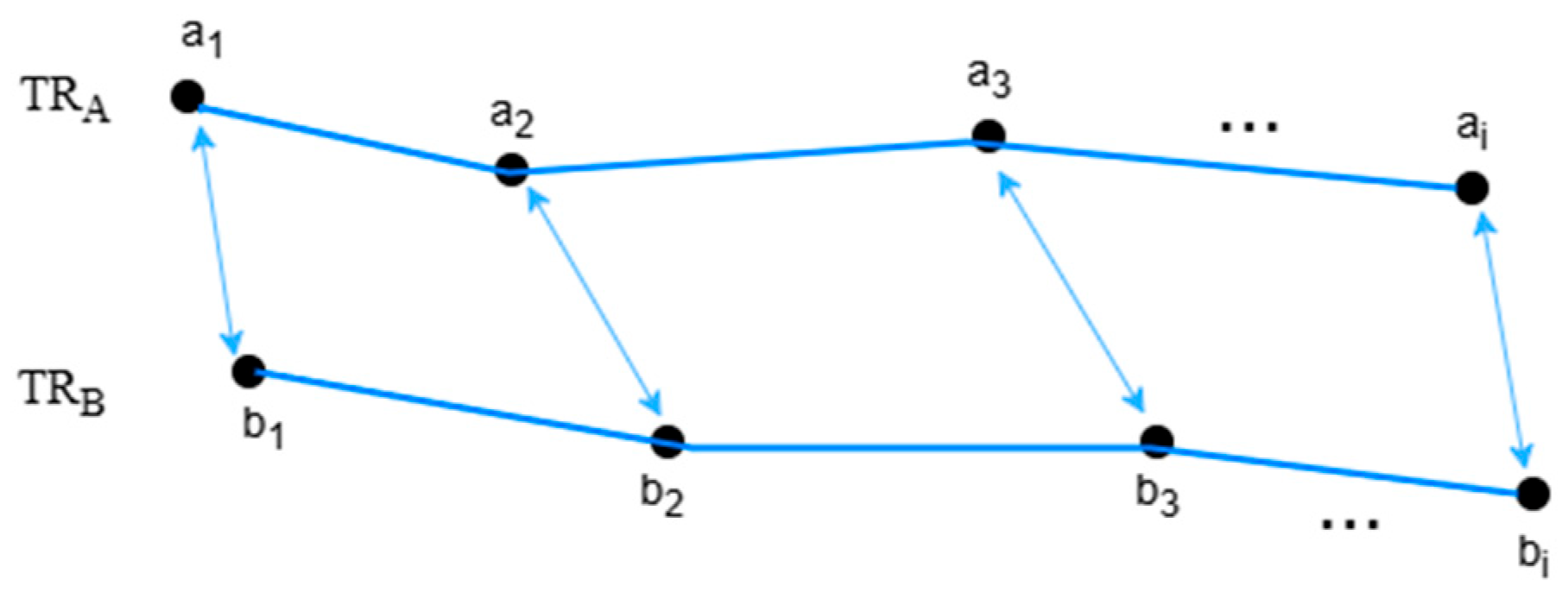
The Hausdorff distance provides a mathematical measure of the distance between two sets within a metric space [41]. It operates by measuring the extent to which each point of one set approximates some point in the other set, with its fundamental principle being the computation of the supremum of all infima of distances between points in the two sets. Formally, the Hausdorff distance from set A to set B is defined as the supremum over all points in A of the infimum of distances to points in B. A small Hausdorff distance indicates that every point of one set is in close proximity to some point in the other set, reflecting strong similarity between the sets. This property makes the Hausdorff distance particularly valuable for assessing the similarity between ship trajectories. Figure 4 presents diagram of Hausdorff distance.
Consider two trajectories: Trajectory: A = { a 1 ,   a 2 ,   ,   a m } , where each point a i = x i , y i , t i represents the ship’s position x i , y i at time t i . Similarly, Trajectory B = { b 1 ,   b 2 ,   ,   b n } , where b j = x j , y j , t j . The directed Hausdorff distance from trajectory A to B, denoted h ( A , B ) , is then defined as:
h A , B = m a x a A m i n b B d a , b
where d ( a , b ) denotes the Euclidean distance between points a and b in two-dimensional space:
d a , b = x i x j 2 + y i y j 2
The bidirectional Hausdorff distance serves as the principal metric for quantifying the overall spatial similarity between two ship trajectories. This measure combines both directed Hausdorff distances to ensure a comprehensive comparison of the two trajectories. The bidirectional Hausdorff distance is formally defined as:
H A , B = m a x h A , B , h B , A
This distance represents the maximum of the two directed Hausdorff distances, effectively capturing the worst-case mismatch between the two point sets.

2.3.3. KD-Tree Algorithm

Owing to the substantial volume of ship trajectory data coupled with the algorithm’s high time complexity, the computation of Hausdorff distance is often computationally expensive. The KD-Tree, a spatial partitioning data structure, enables efficient organization of points in k-dimensional space and facilitates rapid nearest neighbor search as well as range queries [42]. With an average query complexity of O log n , the KD-Tree algorithm markedly accelerates Hausdorff distance calculations by leveraging spatial indexing and pruning strategies.
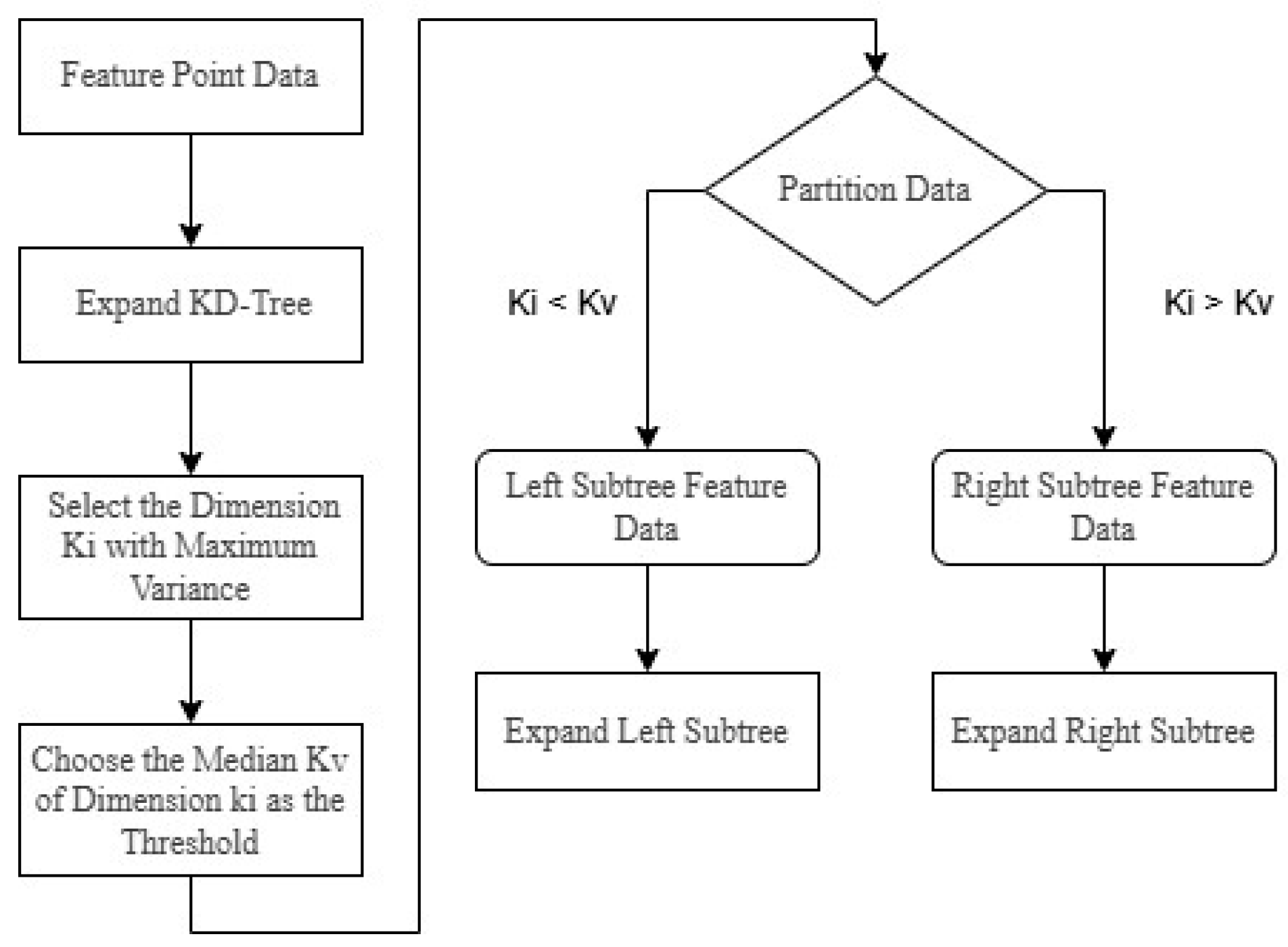
In the conventional computation of Hausdorff distance, the minimum distance from every point in one trajectory set to the other set must be calculated, resulting in an overall time complexity of O m n . For large-scale ship trajectory data, this approach entails substantial computational overhead, thereby impairing the algorithm’s practical efficiency. Thus, employing the KD-Tree algorithm to index the point sets can effectively reduce the time complexity and enhance overall computational efficiency. The overall algorithm flow is illustrated in Figure 5.

2.4. Informer Model

In late 2017, Google researchers published a seminal paper, which introduced the Transformer architecture based on a self-attention mechanism [24]. Unlike traditional recurrent neural networks (RNNs), the Transformer does not rely solely on previous hidden states to compute the current output. Instead, it employs self-attention to weigh all input elements simultaneously, allowing it to focus selectively on relevant information, mitigate data loss, and enhance parallel processing capabilities. The model has achieved remarkable success in time series forecasting. However, subsequent research has revealed several limitations of the Transformer in time series applications, including the high computational complexity and memory usage of its attention mechanism, as well as inherent constraints of the encoder–decoder architecture.
To address these issues, Zhou et al. [30] introduced the Informer in 2021, an enhanced Transformer-based model designed for more efficient sequence prediction. Its main improvements include the following:
(1)
ProbSparse self-attention: This mechanism significantly reduces the time complexity of standard self-attention by sparsifying the attention matrix.
(2)
Self-attention distilling: This technique reduces layer dimensionality and parameter count while emphasizing salient features, improving efficiency in long-sequence processing.
(3)
Generative decoder: Unlike traditional step-by-step decoders, this variant generates the entire output sequence in a single forward pass, reducing error accumulation and improving efficiency.
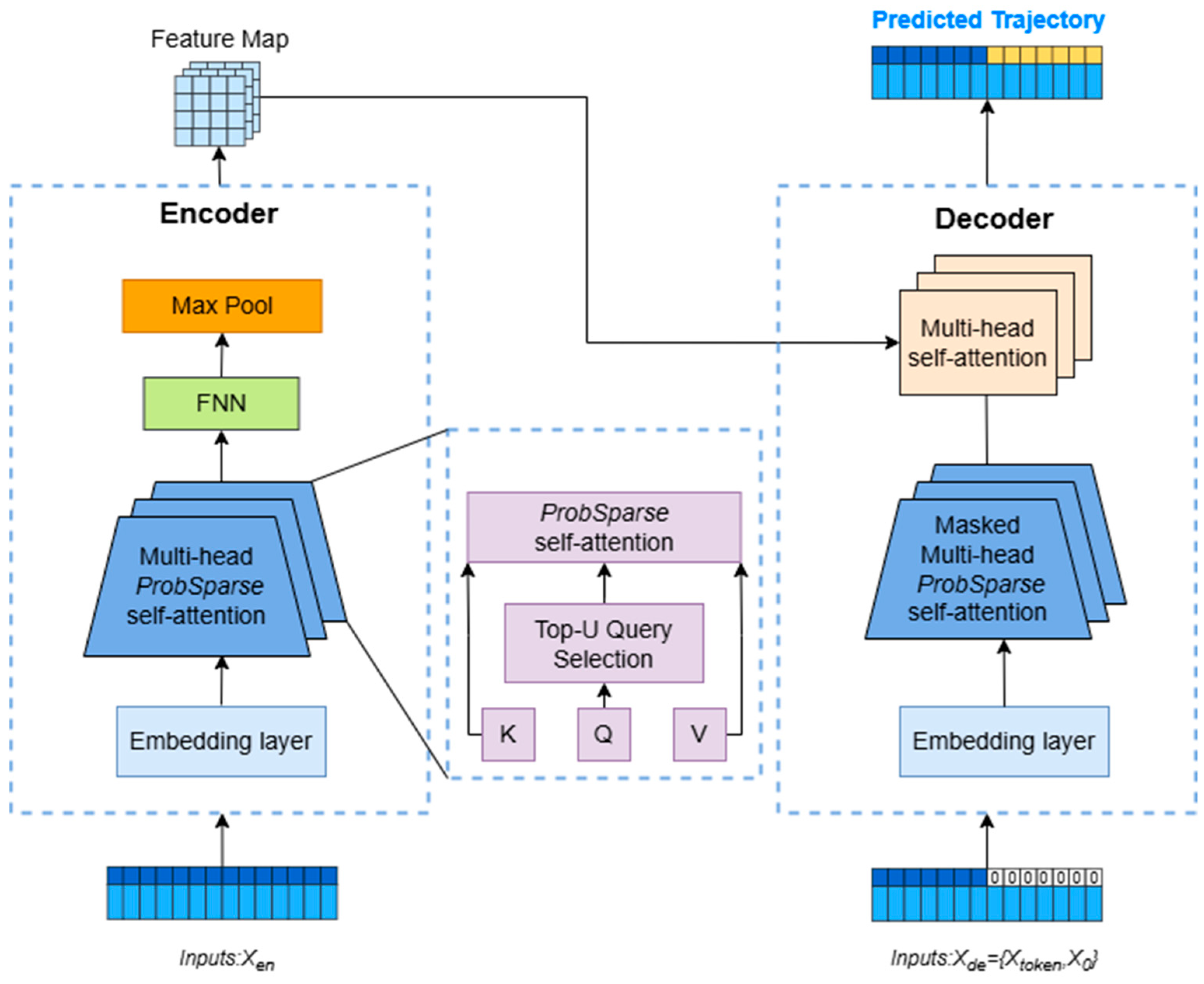
The Informer model comprises an embedding layer, encoder, decoder, and fully connected layer. The encoder captures long-term dependencies in historical sequences, while the decoder generates the target output. The overall architecture is illustrated in Figure 6.

2.4.1. Embedding Layer

The embedding layer in the Informer model transforms the raw input sequence into a latent representation that is interpretable and processable by the model. When processing time series data, the embedding layer must not only capture feature information at individual time points but also incorporate positional and temporal context from the sequence, which is essential for modeling dynamic variations and temporal dependencies. The embedding module comprises three components:
Scalar projection: Applies one-dimensional convolution operations to project variables such as longitude, latitude, course, and speed at time t into a higher-dimensional space.
Local time stamp embedding: Captures the ordinal information of the input sequence by employing a positional encoding scheme similar to the original Transformer, reintegrating positional information into the input by assigning a unique vector to each time step. The positional encoding is computed as follows:
P E P p o s , 2 i = sin P p o s 1000 2 i d
P E P p o s , 2 i + 1 = cos P p o s 1000 2 i d
where P E denotes positional encoding, P p o s indicates the position index in the sequence, d is the embedding dimension, and i represents the dimension index. Equations (5) and (6) correspond to the encoding for even and odd indices, respectively.
Global time stamp embedding: Encodes absolute temporal information (e.g., hour of day, day of week) to capture periodic patterns and temporal context within the trajectory data.

2.4.2. Encoder

The encoder is designed to capture long-term dependencies within input trajectory sequences and primarily consists of a multi-head ProbSparse self-attention module followed by a self-attention distilling module.
(1)
ProbSparse Attention Mechanism
The conventional self-attention mechanism computes attention weights by measuring the similarity between Query and Key vectors, subsequently performing a weighted summation of the Value vectors to produce the final output. The operation is formally defined as:
A Q , K , V = s o f t m a x Q K T d V
where d denotes the input dimension, and Q , K , V represent the Query, Key, and Value matrices, respectively, each of dimension d. Here, K and V are paired, while Q is used to query against K . The softmax function serves as the activation function. The attention coefficient for the i-th query is given by Equation (8):
A q i , K , V = j k q i , k j l k q i , k l ν j = E p k j q i ν j
where p ( k j q i ) = k ( q i , k j ) l k ( q i , k l ) , and k ( q i , k j ) selects e x p ( q i k j T d ) as the asymmetric exponential index.
Although the aforementioned method effectively captures the relative importance between vectors, it requires a substantial number of dot product operations, resulting in high computational complexity that adversely impacts prediction performance. Empirical studies have revealed that only a limited subset of dot product operations contribute significantly, and the distribution of self-attention probabilities exhibits sparsity. To address this, the Informer model incorporates the Kullback–Leibler (KL) divergence to measure the similarity between the attention probability distribution of a Query and the uniform distribution. The sparsity measure for the i-th Query is formally expressed by Equation (9):
M q i , K = l n j = 1 L K e q i k j T d 1 L K j = 1 L k q i k j T d
where the term l n j = 1 L K e q i k j T d represents the log-sum-exp of the scaled dot products between q i and all Keys, and 1 L K j = 1 L k q i k j T d denotes their arithmetic mean. To reduce computational cost, upper and lower bounds are applied to M q i , K , simplifying the expression to Equation (10):
M ¯ q i , K = m a x j q i k j T d 1 L K j = 1 L K q i k j T d
Subsequently, only the top U queries—those with the highest M values—are selected to compute the attention scores. This selection process yields the final ProbSparse self-attention mechanism:
P _ A ( Q , K , V ) = s o f t m a x Q ¯ K T d k V
where Q ¯ is a sparse matrix comprising only the top-U queries under the sparsity measure M ¯ . This refined approach allows the model to concentrate its computational resources on the most influential trajectory points—such as moments of speed change or course alteration—drastically reducing computational complexity while preserving predictive performance.
(2)
Self-Attention Distilling
To reduce potential redundancy in feature information following the self-attention process, self-attention distilling is employed to extract the most salient features, thereby decreasing the complexity of the feature representation. This is achieved by inserting a convolutional pooling layer between consecutive self-attention modules to perform feature down-sampling. The transformation from layer j to layer j+1 is defined as follows:
X j + 1 t = M a x P o o l E L U C o n v 1 d X j t A B
where X j t A B denotes the output from the multi-head sparse self-attention mechanism, M a x P o o l refers to the max-pooling operation, E L U denotes the Exponential Linear Unit activation function, and C o n v 1 d indicates the one-dimensional convolution operation.

2.4.3. Decoder

Each decoder block in the Informer model comprises a masked multi-head ProbSparse self-attention layer, a multi-head self-attention layer, and a fully connected layer. The decoder input is formed by concatenating two components: the output from the encoder and the embedded decoder input, where the latter half of the decoder input is masked with zeros. This is formally expressed in Equation (13):
X d e t = C o n c a t X t o k e n t , X 0 t R L t o k e n + L y × d m o d e l
where X d e t  t—denotes the decoder input sequence, X t o k e n t R ( L t o k e n × d m o d e l ) represents the initial token sequence, X 0 t R L y × d m o d e l is the placeholder-masked prediction sequence (with zeros masking the latter half), L t o k e n is the length of the initial token sequence, and L y is the length of the prediction sequence.
Furthermore, the Informer’s decoder enhances the traditional step-by-step decoding approach by adopting generative-style inference. This allows the entire predicted trajectory sequence to be generated in a single forward pass, thereby reducing prediction time and enhancing accuracy.

2.5. Whale Optimization Algorithm

The Informer model demonstrates strong performance in multi-step and long-term ship trajectory prediction [30]. However, achieving high prediction accuracy across diverse trajectory patterns and varying prediction horizons often requires careful configuration of key hyperparameters. Manual hyperparameter tuning is not only time-consuming but also often yields suboptimal results. Therefore, employing an optimization algorithm to automatically identify optimal hyperparameters for specific trajectory patterns and prediction lengths is essential.
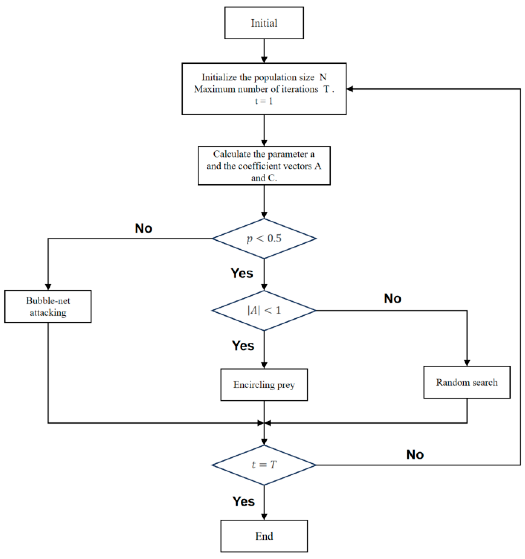
The Whale Optimization Algorithm (WOA) is a metaheuristic algorithm known for its strong optimization capabilities, rapid convergence, and simple structure, with demonstrated effectiveness across various domains [36,37]. WOA simulates the collective hunting behavior of humpback whales, particularly their distinctive “bubble-net” feeding strategy. Its underlying principle involves finding optimal solutions by emulating the self-organizing and adaptive characteristics of whale pod behavior. The algorithm primarily operates through three key phases: encircling prey, bubble-net attacking, and random search. The overall workflow of WOA is illustrated in Figure 7.
The mathematical formulation of the Whale Optimization Algorithm (WOA) operates through the following principles:
(1)
Encircling prey phase: In nature, humpback whales can locate prey and encircle it. In optimization problems, where the global optimum is unknown a priori, the algorithm treats the current best solution as the target prey’s estimated position. Once this reference is established, other search agents update their positions toward it, modeled by
X t + 1 = X * t A × D
D = C × X * t X t
where X * t denotes the position of the best solution found at iteration t , X t and X t + 1 are the current and next positions of a search agent, D represents the enclosure distance, and A and C are coefficient vectors calculated as follows:
A = 2 × a × r 1 a
C = 2 × r 2
a = 2 2 t T
where r 1 and r 2 are uniformly distributed random numbers in the range [0, 1], whose primary role is to introduce necessary stochasticity into the search process, aiding the population in escaping local optima and facilitating global exploration. And a is a control parameter that decreases linearly from 2 to 0 over the course of the total iterations T .
(2)
Bubble-net attacking phase: This phase models the spiral attacking maneuver of humpback whales by establishing a spiral update equation between the whale and the prey, formulated mathematically as:
X t + 1 = D * × e b l × cos 2 π l + X * t
D * = X * t X t
where D * represents the distance between the i-th whale individual and the optimal individual, b is a constant parameter used to control the shape of the spiral, and l is a random number between [0, 1].
In addition, to simultaneously simulate the contraction encirclement mechanism and spiral update mechanism of whales, it is generally assumed that the two mechanisms have equal execution probabilities, whose mathematical expression is as follows:
X t + 1 = X * t A × D , p < 0.5 D * × e b l × c o s 2 π l + X * t , p 0.5
(3)
Random search phase: To prevent the population from converging prematurely on local optima, the algorithm incorporates a random search strategy that enhances its exploration capabilities. This phase is mathematically represented as follows:
X t + 1 = X r a n d t A × D
D = C × X r a n d t X t
where X r a n d t denotes the position vector of a randomly selected whale from the current population. It is important to note that the mathematical formulations for both the encircling prey and random search phases are similar. The choice between these two behaviors is contingent upon the value of the coefficient A . Specifically, the encircling prey behavior is executed when A < 1 , whereas the search for prey is triggered when A 1 .

3. Experimental Results and Analysis

In this section, we first present experimental results for the preparatory stages—specifically, data cleaning and trajectory clustering—as described in the preceding methodology, since these steps critically influence subsequent model prediction performance. We then evaluate the WOA-Informer model using trajectory data from three distinct pattern types, comparing its performance against multiple baseline methods to assess its generalization capability and predictive accuracy. The experimental setup used in this study is summarized in Table 1.

3.1. Data Preprocessing Analysis

This study focuses on a designated water area within the Qingdao Port region (120.17° E–120.34° E, 35.96° N–36.06° N). This region exhibits several notable characteristics: First, it serves as a major access channel to Huangdao Qianwan Wharf, where ships undergo berthing operations, resulting in diverse navigational trajectory patterns. Second, the area contains abundant ship trajectory data, offering substantial support for this research. Moreover, the waterway exhibits stable traffic flow, favorable hydrological conditions, and smooth water movement, making it an ideal environment for validating model prediction performance. A sample of the ship AIS data is provided in Table 2.
This paper focuses specifically on the trajectory prediction of large merchant ships, excluding auxiliary vessels such as tugs and engineering ships. Drawing on the actual conditions of the water area at Qianwan Wharf in Qingdao Port, this study collected trajectory data from ships traveling from their inbound approach to final berthing between 1 October and 15 November 2024. Following the data preprocessing method detailed in Section 2, we ultimately obtained 207 valid ship trajectories, which contain 76,506 high-quality trajectory points.
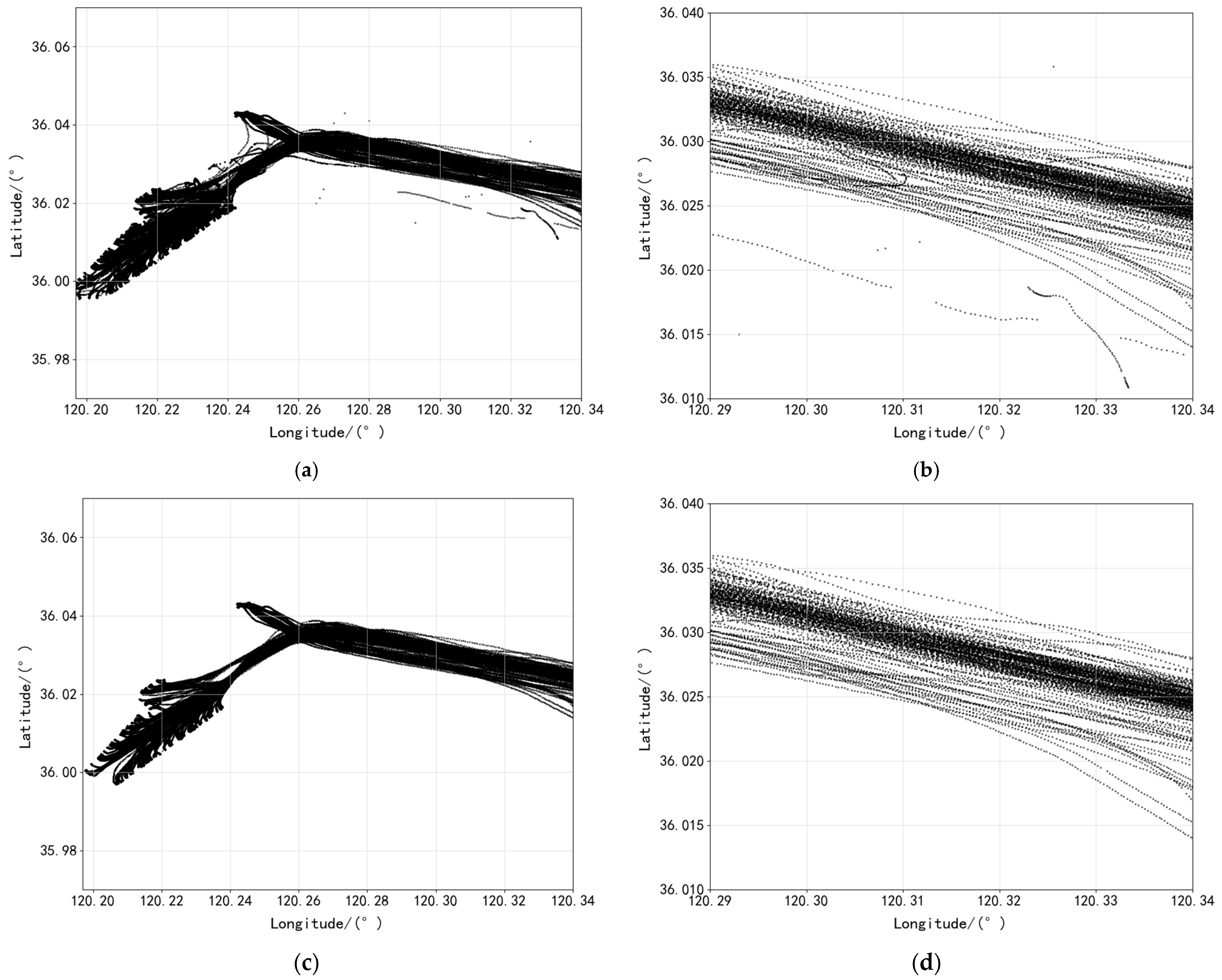
Figure 8a illustrates the spatial distribution of raw AIS trajectory data, revealing that some trajectories exhibit obvious noise and outliers. Figure 8c presents the results following rigorous data cleaning, with disorganized trajectories and abnormal trajectories that violate ship kinematic characteristics having been effectively eliminated. This comparison clearly demonstrates that the preprocessed trajectory data more accurately reflects the actual trajectory characteristics of ships, thereby laying a reliable data foundation for subsequent trajectory clustering and prediction analysis.

3.2. Trajectory Clustering Analysis

Visual analysis of the preprocessed ship trajectory data, presented in Figure 8b, indicates that the navigation trajectories of large merchant ships display pronounced multi-modal distribution characteristics. If all trajectory data are amalgamated and fed directly into the prediction model, the inherent differences among distinct patterns may diminish the model’s learning efficacy. Therefore, this study employs a density-based trajectory clustering approach to categorize ship trajectory patterns. Extracting representative trajectory data for each pattern can significantly enhance the relevance of model training and improve prediction accuracy.
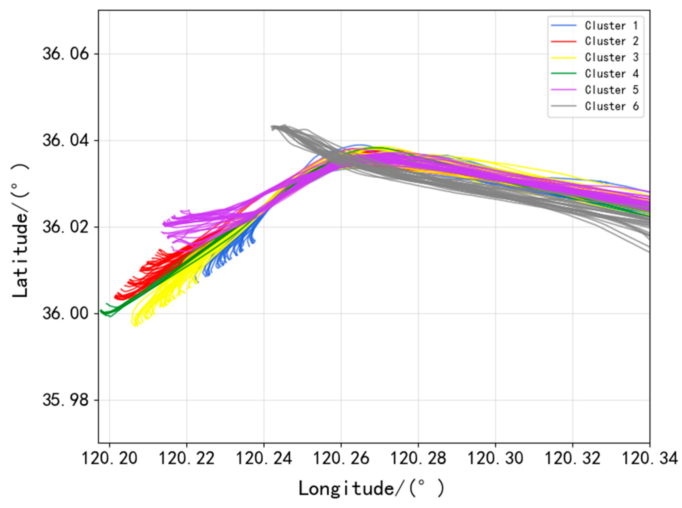
For clustering parameter selection, the core parameters of the DBSCAN algorithm were determined via an adaptive parameter combination method [43], resulting in ε = 0.003 and M i n P t s = 5 . This parameter set effectively identifies trajectory clusters sharing similar spatial characteristics while avoiding the misclassification of discrete points as valid clusters. The resulting clustering effect is illustrated in Figure 9.
As illustrated in Figure 9, the Hausdorff distance-based DBSCAN algorithm successfully clusters ship trajectories within the Qianwan Wharf area of Qingdao Port. The algorithm effectively identifies six distinct trajectory clusters, each exhibiting a spatial distribution that aligns closely with actual ship navigation patterns observed in the port. Specifically, clusters 1–4 exhibit broadly similar navigation characteristics, all representing typical inbound patterns involving a single turn. Among these, vessels in cluster 1 primarily berth in the upper-right region of the wharf, executing a relatively large turning maneuver. Cluster 5 represents another common pattern, wherein vessels must complete two distinct turns before berthing in the upper-left zone. Cluster 6 is notably unique, comprising trajectories of large oil tankers that follow an almost straight-line path directly to the dedicated tanker wharf in the upper area.
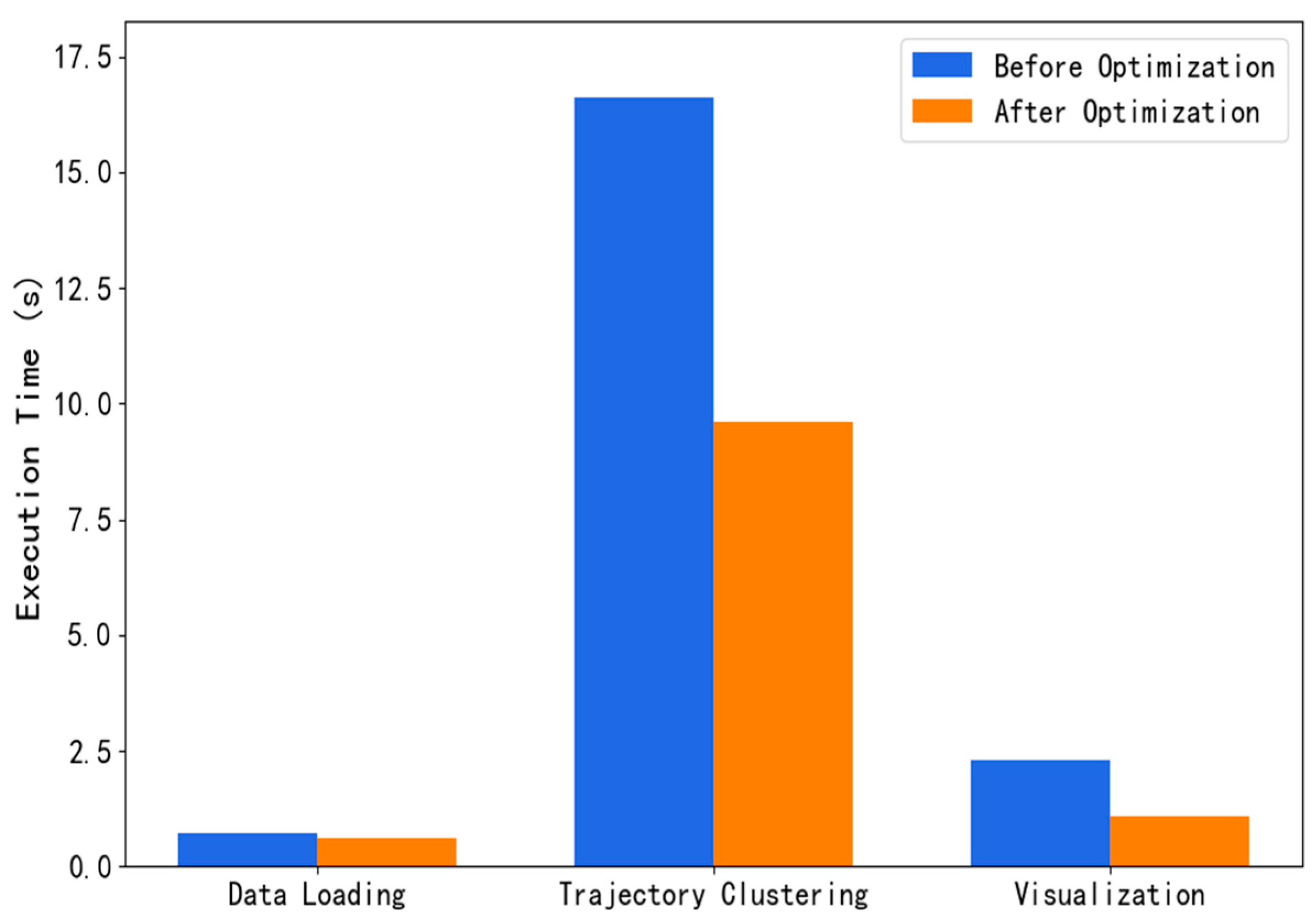
To improve clustering efficiency, the KD-Tree algorithm was incorporated to significantly accelerate Hausdorff distance computation through spatial indexing and pruning strategies. Additionally, the CuPy library was employed to compute nearest-neighbor distances for all points in parallel on the GPU, further reducing clustering time. The distribution of overall execution times is presented in Figure 10.
As evident from the figure above, the processing time for both trajectory clustering and visualization is substantially reduced following optimization via the KD-Tree algorithm and parallel computing. Notably, the trajectory clustering stage exhibits the most substantial reduction, with processing time decreasing from 16.5967 s to 9.6142 s, corresponding to a 57.9% improvement in efficiency. The overall execution time is reduced from 19.7785 s to 11.2802 s, achieving a comprehensive efficiency gain of 57%. These results confirm the efficacy of KD-Tree for spatial index construction and demonstrate the suitability of parallel computing for processing large-scale trajectory data.

3.3. Prediction Result Analysis of WOA-Informer Model

3.3.1. Sample Dataset Construction and Evaluation Indicators

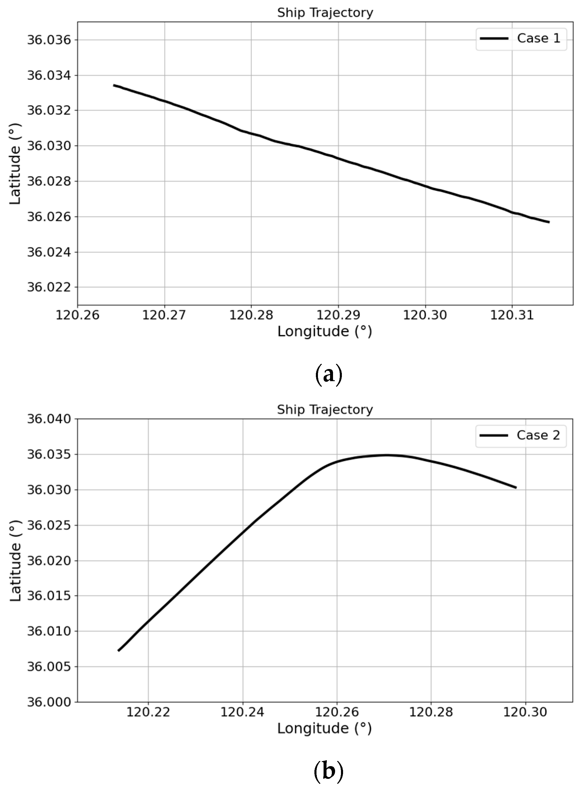
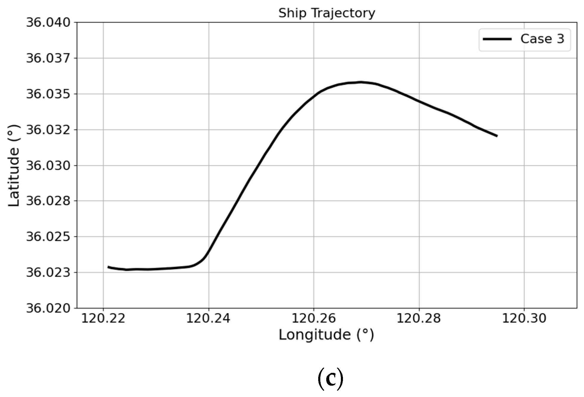
To comprehensively evaluate the optimization performance of the Whale Optimization Algorithm (WOA), this study selects the three most representative trajectory clusters from the clustering results as experimental subjects. These three clusters correspond to three typical vessel navigation patterns in port waters: (1) straight-line navigation; (2) navigation with a single distinct turn; (3) navigation involving successive distinct turns. This selection strategy ensures the verification process is both comprehensive and representative. Figure 11 presents three trajectory patterns.
The preprocessed high-quality dataset was subsequently resampled. Given the dense ship traffic and complex navigational conditions in port waters, the resampling time interval was set to 10 s. This interval preserves trajectory feature integrity while effectively capturing vessel navigation characteristics in restricted waters.
During the feature engineering stage, longitude, latitude, speed over ground (SOG), and course over ground (COG) were selected as input features to comprehensively characterize vessel motion states. To enhance model generalization and mitigate the effects of varying data scales and units, min-max normalization was applied to the dataset prior to model input. The normalization is performed as follows Equation (24):
X = X X m i n X m a x X m i n
where X represents each feature value, X m i n denotes the minimum value of the feature, and X m a x represents the maximum value.
To quantify the prediction performance of the ship trajectory prediction model, a set of evaluation metrics is employed. Four objective evaluation metrics are selected: Root Mean Square Error (RMSE), Mean Absolute Error (MAE), Mean Absolute Percentage Error (MAPE), and Haversine distance. While MAE provides a straightforward single-value assessment, its utility is primarily realized when comparing different models. In contrast, RMSE more directly characterizes the prediction quality of the model; a lower RMSE value corresponds to higher predictive accuracy [44]. The Haversine distance metric calculates the great-circle distance between the actual and predicted points, offering a more intuitive representation of the model’s performance by translating error into a tangible geographical displacement [31]. The formulas for these four evaluation metrics are as follows:
R M S E = 1 m i = 1 m ( y 𝚤 ^ y i ) 2
M A E = 1 m i = 1 m y ^ i y i
M A P E = 1 m i = 1 m y 𝚤 ^ y i y i
H A V = 2 R a r c s i n s i n 2 ( ϕ ¯ ) + c o s ( ϕ 1 ) c o s ( ϕ 2 ) s i n 2 ( λ ¯ )
In these formulae, m represents the total number of samples, y 𝚤 ^ denotes the model’s predicted value, and yi is the corresponding actual trajectory value. For the Haversine distance, R signifies the Earth’s radius, while ϕ ¯ and λ ¯ are the midpoints for latitude and longitude differences, calculated as | ϕ 2 ϕ 1 | / 2 and | λ 2 λ 1 | / 2 , respectively. Here, ϕ 1 and λ 1 refer to the predicted longitude and latitude, whereas ϕ 2 and λ 2 correspond to the actual longitude and latitude.

3.3.2. WOA Hyperparameter Selection and Optimization Results

The selection of hyperparameters critically determines the prediction performance of the model. The hyperparameter optimization process integrating the WOA with the Informer model comprises three key components: the WOA itself, the Informer model architecture, and the sample dataset. Initially, the Informer network decodes the input parameters from the WOA to initialize its hyperparameters. The sample dataset is partitioned into training, validation, and test sets with an 8:1:1 ratio, where the training set is utilized to train the Informer network. The validation set then serves to fine-tune the model’s hyperparameters, with the mean square error between predictions and ground truth being returned to the WOA as the fitness value. Guided by this fitness value, the WOA optimizes the hyperparameters by iteratively updating the optimal position coordinates of humpback whale individuals, ultimately yielding an optimal set of network hyperparameters.
The control parameters for the Whale Optimization Algorithm were determined through systematic sensitivity analysis of population characteristics. A series of experiments evaluated combinations of population sizes ranging from 5 to 50 and maximum iteration counts between 10 and 100 to assess their impact on convergence behavior. Analysis revealed that a population size of 15 combined with 40 maximum iterations provided the optimal balance—maintaining robust global search capability while demonstrating accelerated convergence and enhanced optimization stability. This configuration effectively reconciles computational efficiency with thorough search coverage.
The optimization objectives were established through a combined approach of a literature review and an empirical validation. Building on parameter recommendations for the Informer architecture from reference [31], we conducted multiple controlled experiments to systematically assess hyperparameter sensitivity in ship trajectory prediction. Our analysis identified five particularly influential hyperparameters—learning rate, batch size, encoder layers, decoder layers, and dropout rate—that significantly impact prediction accuracy and generalization capability. These parameters were consequently designated as optimization targets for WOA, enabling automated discovery of optimal configurations. The corresponding search ranges for these hyperparameters are summarized in Table 3. The value ranges for these optimized hyperparameters are presented in Table 4.

3.3.3. Prediction Results of WOA-Informer Model

To comprehensively evaluate the prediction performance of the WOA-Informer model, this study utilizes trajectory data from three distinct datasets. Each dataset is partitioned into training, validation, and test sets using an 8:1:1 ratio, with one trajectory randomly selected from the test set as the target trajectory for demonstration. (It should be noted that while our experiments encompass multiple trajectories across six trajectory clusters, only three are randomly selected here for experimental demonstration).
The initial WOA-Informer model architecture comprises two encoder layers and one decoder layer, with additional parameters including a learning rate of 0.001, batch size of 32, and dropout rate of 0.1. The model employs Gelu as the activation function and Adam as the optimizer [45]. To validate the effectiveness of the proposed WOA-Informer approach, several representative baseline models were selected for comparison. These include: the CNN-BILSTM model, representing traditional RNN architectures; the Transformer model with its encoder–decoder framework; and the original Informer model prior to optimization. The primary parameter configurations for these baseline models are summarized in Table 5.
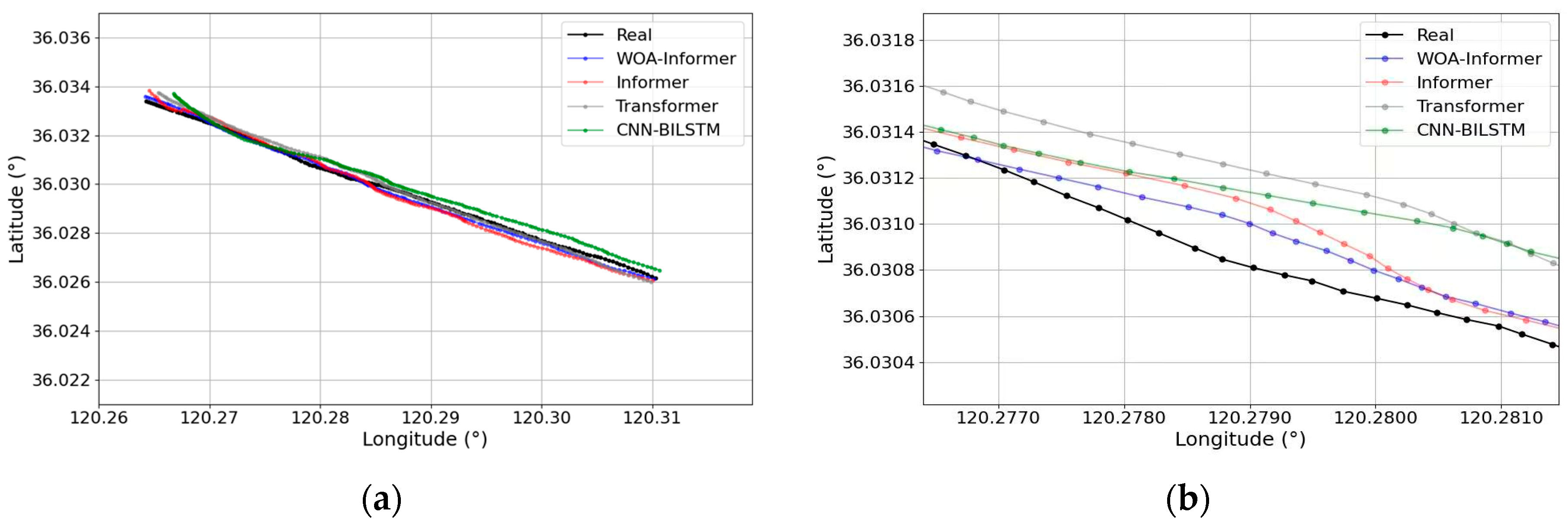
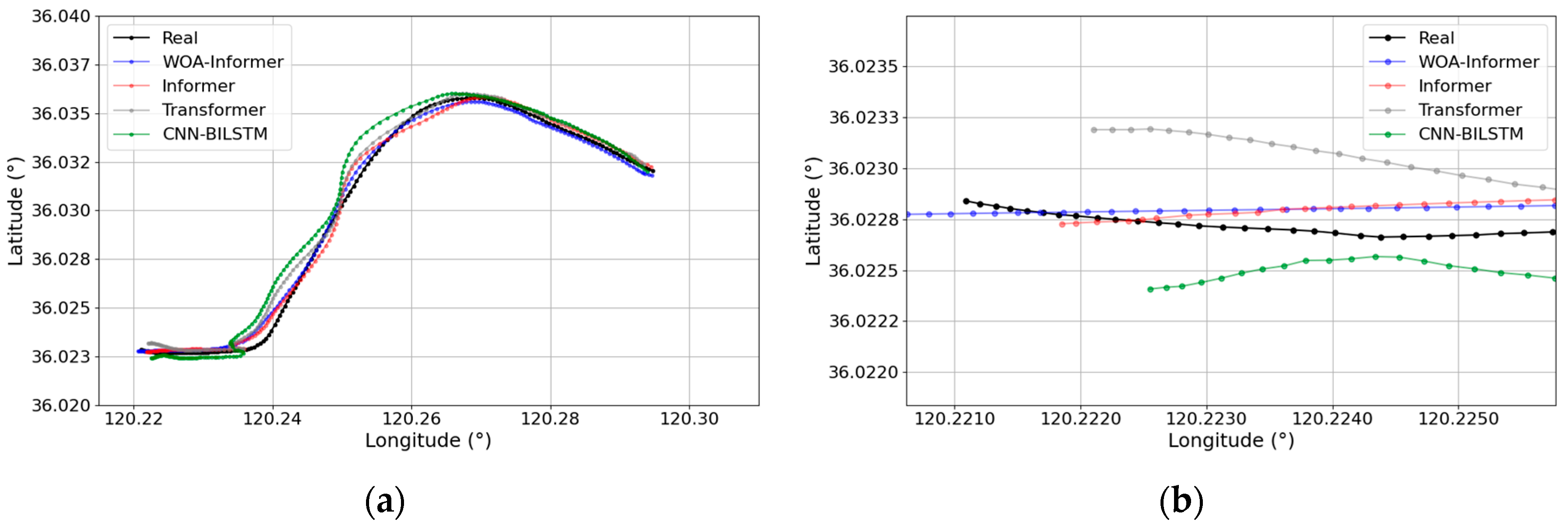
To assess the robustness and accuracy of the proposed model for medium-to-long-term and multi-step trajectory prediction, the first 20 trajectory points were used as input to predict the subsequent 20 points. This process generated a total of 180 predicted trajectory steps for evaluation. The prediction results of each model across the three trajectory patterns are presented in Figure 12, Figure 13 and Figure 14.
The visualization of the prediction results reveals that under the nearly straight trajectory pattern, all models demonstrate a good fit to the ship’s motion trajectory. The WOA-optimized Informer model most closely approximates the actual trajectory, whereas the other models exhibit varying degrees of divergence in the final prediction stage, with CNN-BILSTM showing the most significant deviation.
For trajectories featuring a single distinct turn, all models initially produce predictions close to the actual values, but significant discrepancies emerge following the turn. Each baseline model begins to diverge from the actual trajectory after the turn, and the deviation distance of the CNN-BILSTM model gradually increases with the number of prediction steps. Although both the Informer and Transformer models show noticeable deviations, these do not substantially increase with additional prediction steps, underscoring the importance of the attention mechanism for learning long-term dependencies in trajectory sequences. The WOA-Informer model exhibits minor fluctuations immediately after the turn but gradually converges toward the actual trajectory as prediction steps increase. This improvement primarily stems from the WOA’s optimization of Informer hyperparameters, which yields a more accurate parameter set, identifies key attributes affecting prediction accuracy, and mitigates the blindness of manual parameter setting.
In the case of continuously turning trajectories, all models perform well initially but begin to diverge significantly during the first turn. While most baseline models deviate from the actual trajectory to varying degrees, the WOA-Informer model maintains a close fit even during turns. During the second turn, the deviation in the predicted trajectories of the baseline models continues to increase, with some even exhibiting unrealistic ship motion retracing. The WOA-optimized Informer model also shows increased deviation from the actual trajectory during the second turn, but this remains within acceptable error limits, and the model quickly converges back to the actual trajectory after the turn. These results further validate the crucial role of the WOA in enhancing ship trajectory prediction.
For a more objective evaluation of the model’s predictive performance, this study computed the evaluation metrics for each model using Equations (25)–(28), with the results detailed in Table 6, Table 7 and Table 8. Under trajectory pattern 1, the WOA-Informer model achieved the best performance, demonstrating a 63.1% reduction in RMSE compared to the CNN-BILSTM model, 39.3% compared to the Transformer model, and 23.5% compared to the unoptimized Informer model. These improvements indicate a significant enhancement in trajectory fitting accuracy.
For trajectory pattern 2, while the Transformer model slightly outperformed the original Informer model, the optimized Informer model still delivered the best predictive results. Specifically, it reduced RMSE by 58.4% compared to CNN-BILSTM, 10.4% compared to Transformer, and 14.0% compared to the baseline Informer model. In terms of average Haversine distance, the WOA-Informer model achieved only 69.19 m—27.8% lower than that of the Informer model—indicating stronger robustness in complex trajectory prediction.
Under the third trajectory pattern, the WOA-Informer model showed even more substantial improvements, outperforming all baseline models across all four evaluation metrics. Compared with the unoptimized Informer, it reduced RMSE by 31.8%, MAE by 28.6%, MAPE by 13.5%, and average Haversine distance by 32.4%, further verifying its advantages in complex trajectory prediction.
A comprehensive analysis of the prediction results across the three trajectory patterns reveals that the CNN-BILSTM model performs relatively poorly in multi-step and medium-to-long-term predictions. This limitation may be attributed to the absence of an attention mechanism, which restricts its ability to capture long-range dependencies in trajectory sequences. Both the Transformer and Informer models demonstrate superior performance with comparable prediction accuracy, yet they exhibit noticeable fluctuations around turning points. This phenomenon suggests that suboptimal network parameters may become trapped in local optima, thereby limiting the models’ capacity to effectively capture maneuvering characteristics. The WOA-Informer model achieves the best performance across all evaluation metrics in every test scenario, conclusively validating the effectiveness of the WOA for hyperparameter optimization. Its global search capability significantly enhances the model’s adaptability to complex navigation patterns, demonstrating robust performance in challenging trajectory prediction tasks.
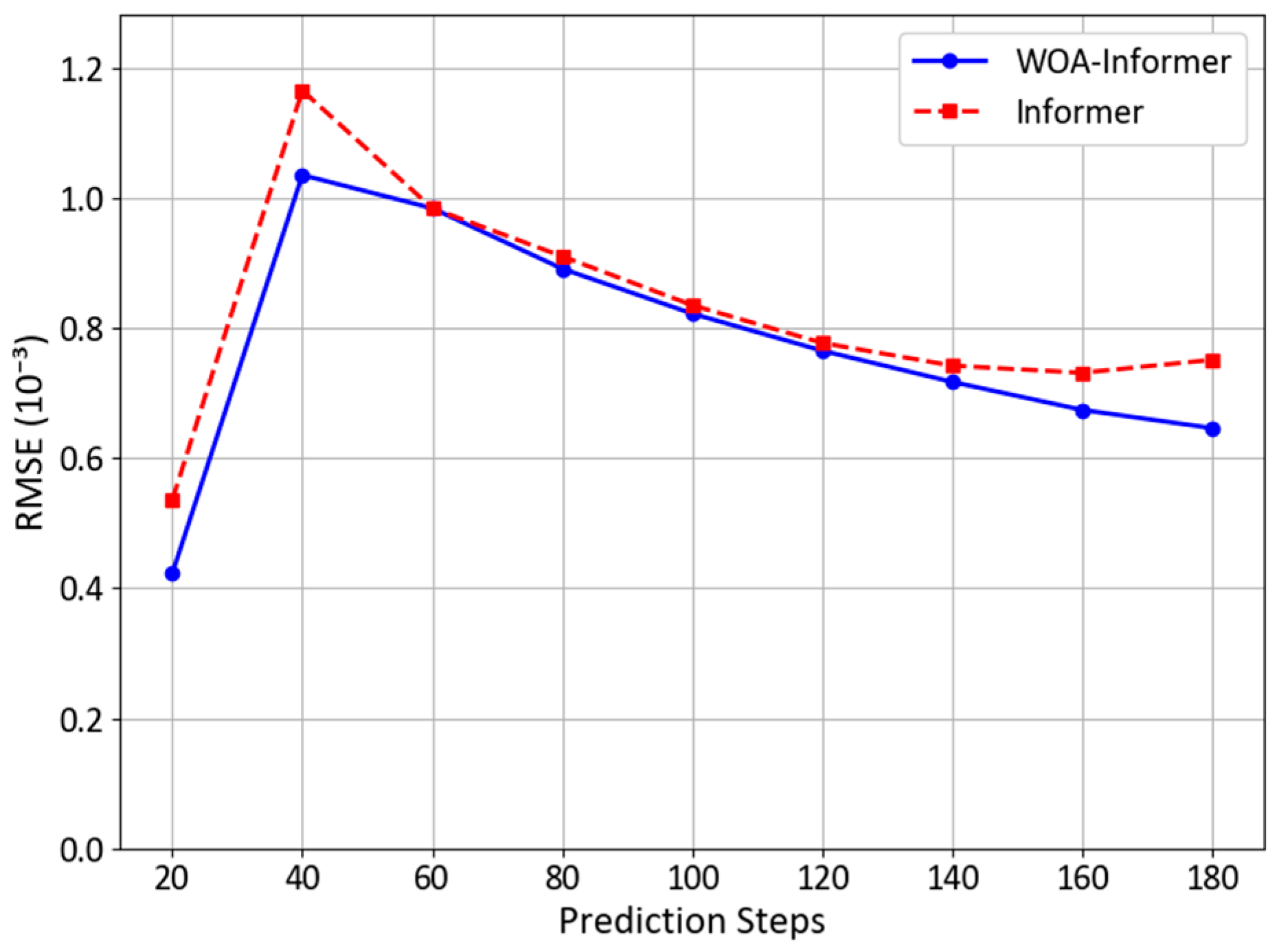
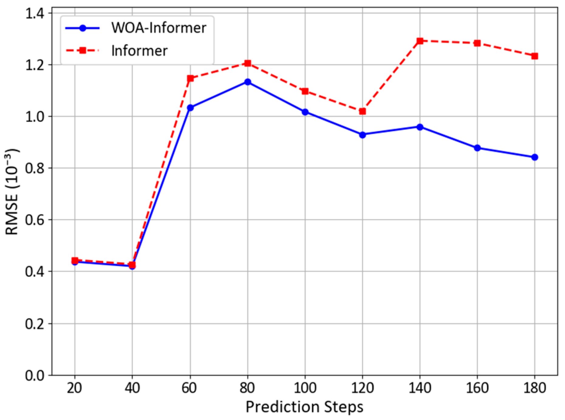
To gain deeper insights into how the WOA optimizes the hyperparameters of the Informer model, this study evaluates the stage-wise prediction performance across three typical trajectory patterns. Specifically, model performance is assessed at 20-time-step intervals using RMSE as the evaluation metric throughout the entire prediction cycle. The detailed comparative results are presented in Figure 15, Figure 16 and Figure 17.
As evidenced by the aforementioned figures, the WOA-optimized Informer model consistently demonstrates lower RMSE values than its unoptimized counterpart across all stages of trajectory pattern 1, along with reduced error fluctuations, indicating more stable prediction performance. For trajectory pattern 2, the optimized model exhibits lower RMSE values at every stage compared to the pre-optimization version, with a mitigated error increase at the turning point and a rapid error reduction following the turn. Even under the more complex conditions of trajectory pattern 3, the model maintains reduced RMSE values throughout all stages and achieves stable error levels more swiftly after turns, highlighting WOA’s efficacy in handling intricate motion patterns.
These results substantiate the significant role of WOA in enhancing ship trajectory prediction accuracy: it not only comprehensively reduces prediction errors but also markedly improves the model’s adaptability to key motion state changes, aligning predictions more closely with actual navigation scenarios. Particularly during nonlinear motion phases such as turns, the optimized model demonstrates enhanced robustness, which is crucial for ensuring navigation safety.
The computational efficiency comparison presented in Table 9 reveals significant differences in running times among the models. Specifically, across all three trajectory patterns, the Informer model demonstrates the best computational performance, with an average running time of merely 18.477 s—significantly more efficient than the other comparative models. Although the incorporation of WOA increases the running time of the WOA-Informer model, its computational efficiency remains substantially higher than that of both the CNN-BILSTM and Transformer models. Notably, the moderate computational trade-off of the WOA-Informer model is well balanced against its performance gains; while running time increases marginally, the substantial improvement in prediction accuracy renders this additional computational cost highly worthwhile.
In summary, the proposed WOA-Informer model exhibits outstanding comprehensive performance in ship trajectory prediction tasks. Through systematic evaluation on three characteristic trajectory patterns—straight-line, single-turn, and continuous-turn—the model significantly outperforms benchmark models in multi-step and medium-to-long-term prediction tasks. Although the parameter optimization process results in slightly longer running times compared to the baseline Informer model, this remains within an acceptable range. This optimized balance between prediction accuracy and computational efficiency endows the WOA-Informer model with considerable deployment advantages in practical engineering applications, providing reliable technical support for the development of intelligent ships and maritime transportation systems.

4. Conclusions

This paper presents a Whale Optimization Algorithm (WOA)-enhanced Informer model, termed WOA-Informer, designed for high-precision multi-step and medium-to-long-term prediction of ship trajectories. By integrating trajectory clustering techniques with deep learning optimization methods, we establish a comprehensive ship trajectory prediction framework. Experimental validation conducted on AIS data from the Qingdao Port area systematically evaluates the model’s predictive performance across three characteristic trajectory patterns: straight-line, single-turn, and continuous-turn. Comparative analyses with baseline models—including CNN-BILSTM, Transformer, and the standard Informer—demonstrate the superiority of the proposed approach. The research findings indicate that employing WOA to optimize the Informer model’s hyperparameters mitigates the subjectivity of manual parameter selection and alleviates the randomness in parameter configuration. This optimization enables the hybrid model to exhibit significant advantages in prediction accuracy, robustness, and computational efficiency. The specific conclusions derived from this study are as follows:
(1)
Efficiency of trajectory clustering method: Addressing the multimodal characteristics of ship trajectories in port waters, this study employs a DBSCAN clustering algorithm based on Hausdorff distance, successfully identifying six distinct types of ship trajectory clusters. By incorporating a KD-Tree spatial index structure and GPU parallel computing, the computational time of the traditional clustering algorithm is reduced from 16.60 s to 9.61 s, achieving a 57.9% improvement in efficiency.
(2)
Significant improvement in prediction accuracy: The WOA-Informer model delivers optimal predictive performance across all three trajectory patterns. Compared to the unoptimized Informer model, it achieves average reductions of 23.1% in RMSE, 22.4% in MAE, 12% in MAPE, and 27.8% in Haversine distance. Particularly in complex turning scenarios (e.g., Trajectory Pattern 3), the model demonstrates enhanced adaptability to nonlinear motion, with errors converging more rapidly after turns, validating the efficacy of WOA in hyperparameter tuning.
(3)
Balanced computational efficiency optimization: Although introducing the WOA slightly increases the model’s training time, the ProbSparse attention mechanism ensures that its computational efficiency remains significantly higher than that of the CNN-BiLSTM and Transformer models. This balance between accuracy and efficiency enhances the model’s practical applicability for real-world engineering deployment.

4.1. Limitations

Although the proposed WOA-Informer model demonstrates significant advantages in ship trajectory prediction tasks, several limitations warrant further discussion.
From a data standpoint, this study is constrained by its exclusive reliance on AIS data collected from the Qingdao Port area, resulting in limited geographical coverage and insufficient diversity in navigational scenarios. The lack of trajectory data captured during extreme weather conditions further restricts the model’s ability to generalize to such challenging environments. Moreover, the framework predominantly utilizes conventional AIS navigation parameters and does not incorporate multi-source heterogeneous data, such as radar tracks and meteorological information, which could enhance its responsiveness to complex and dynamically changing environmental conditions.
In terms of model architecture, the parameter optimization procedure in the Whale Optimization Algorithm remains computationally intensive, creating implementation barriers for real-time embedded systems with stringent latency constraints. Furthermore, the WOA-Informer’s predominantly data-driven approach lacks explicit encoding of maritime domain knowledge, such as ship collision avoidance norms and collective motion dynamics, potentially compromising prediction reliability in high-density multi-vessel situations. Additionally, the current static clustering methodology shows limited adaptability to evolving ship navigation behaviors, including temporary route modifications that frequently occur in actual maritime operations.

4.2. Future Research

To address these limitations, future research should advance across multiple dimensions. At the data level, efforts should focus on creating cross-regional, multi-scenario benchmark datasets for trajectory prediction—especially those capturing navigation data under special conditions such as extreme weather and emergency collision avoidance. Generative adversarial networks could be leveraged for data augmentation, while deep fusion techniques integrating AIS with radar, satellite remote sensing, and other multi-source data should also be explored.
In terms of model optimization, priority should be given to lightweight design breakthroughs that balance prediction accuracy with computational efficiency, achievable through neural architecture search and model pruning. We recommend adopting an “offline optimization, online deployment” paradigm for scenarios with stringent real-time requirements. This approach involves utilizing historical data to complete the computationally intensive WOA optimization offline, followed by deploying the finalized optimal model with its parameters to the production environment for real-time prediction. Algorithmic innovations may include hybrid strategies that combine WOA with other intelligent optimization algorithms to improve parameter search efficiency, or the adoption of spatiotemporal graph neural networks to better capture interactive relationships among vessels. Future work should also address the growing scholarly demand for uncertainty quantification by integrating probabilistic methods to generate confidence intervals for each trajectory prediction. Such an approach would provide a crucial risk assessment metric to directly inform maritime decision-making processes.

Author Contributions

Conceptualization, H.X.; methodology, J.W. and H.X.; software, J.W.; validation, J.W., S.X. and Z.S.; formal analysis, J.W., H.X. and S.X.; resources, H.X. and J.W.; data curation, J.W. and S.X.; writing—original draft preparation, J.W. and Z.S.; writing—review and editing, H.X. All authors have read and agreed to the published version of the manuscript.

Funding

This research was funded by Research on Supervision Rules of Tianjin Sea Routes (Trial), grant number 3132025635. (supported by the Fundamental Research Funds for the Central Universities).

Data Availability Statement

The raw data supporting the conclusions of this article will be made available by the authors on request.

Conflicts of Interest

The authors declare no conflicts of interest.

References

  1. Seong, N.; Kim, J.; Lim, S. Graph-Based Anomaly Detection of Ship Movements Using CCTV Videos. J. Mar. Sci. Eng. 2023, 11, 1956. [Google Scholar] [CrossRef]
  2. Zhen, R.; Shao, Z.; Pan, J. Advance in character mining and prediction of ship behavior based on AIS data. J. Geo-Inf. Sci. 2021, 23, 2111–2127. [Google Scholar] [CrossRef]
  3. Wang, S.; Nie, H.; Shi, C. A Drifting Trajectory Prediction Model Based on Object Shape and Stochastic Motion Features. J. Hydrodyn. 2014, 26, 951–959. [Google Scholar] [CrossRef]
  4. Qiao, S.; Han, N.; Zhu, X.; Shu, H. A dynamic trajectory prediction algorithm based on Kalman filter. Acta Electonica Sin. 2018, 46, 418–423. [Google Scholar]
  5. Fossen, S.; Fossen, T.I. eXogenous Kalman Filter (XKF) for Visualization and Motion Prediction of Ships Using Live Automatic Identification System (AIS) Data. MIC 2018, 39, 233–244. [Google Scholar] [CrossRef]
  6. Moreira, L.; Vettor, R.; Guedes Soares, C. Neural Network Approach for Predicting Ship Speed and Fuel Consumption. J. Mar. Sci. Eng. 2021, 9, 119. [Google Scholar] [CrossRef]
  7. Bai, W.; Zhang, W.; Cao, L.; Liu, Q. Adaptive Control for Multi-Agent Systems with Actuator Fault via Reinforcement Learning and Its Application on Multi-Unmanned Surface Vehicle. Ocean Eng. 2023, 280, 114545. [Google Scholar] [CrossRef]
  8. Bai, W.; Chen, D.; Zhao, B.; D’Ariano, A. Reinforcement Learning Control for a Class of Discrete-Time Non-Strict Feedback Multi-Agent Systems and Application to Multi-Marine Vehicles. IEEE Trans. Intell. Veh. 2025, 10, 3613–3625. [Google Scholar] [CrossRef]
  9. Wang, Q.; Zhang, Q.; Wang, Y.; Hu, Y.; Guo, S. Event-Triggered Adaptive Finite Time Trajectory Tracking Control for an Underactuated Vessel Considering Unknown Time-Varying Disturbances. Transp. Saf. Environ. 2023, 5, tdac078. [Google Scholar] [CrossRef]
  10. Zhou, H.; Chen, Y.; Zhang, S. Ship Trajectory Prediction Based on BP Neural Network. J. Artif. Intell. 2019, 1, 29–36. [Google Scholar] [CrossRef]
  11. Kim, J.-S. Vessel Target Prediction Method and Dead Reckoning Position Based on SVR Seaway Model. Int. J. Fuzzy Log. Intell. Syst. 2017, 17, 279–288. [Google Scholar] [CrossRef]
  12. Liu, J.; Shi, G.; Zhu, K. Vessel Trajectory Prediction Model Based on AIS Sensor Data and Adaptive Chaos Differential Evolution Support Vector Regression (ACDE-SVR). Appl. Sci. 2019, 9, 2983. [Google Scholar] [CrossRef]
  13. Zhang, M.; Huang, L.; Wen, Y.; Zhang, J.; Huang, Y.; Zhu, M. Short-Term Trajectory Prediction of Maritime Vessel Using k-Nearest Neighbor Points. J. Mar. Sci. Eng. 2022, 10, 1939. [Google Scholar] [CrossRef]
  14. Gao, L.; Wu, j.; Yang, Z.; Xu, C.; Feng, Z.; Chen, J. Long-term Prediction of Ship Trajectories Using TCNformer Based on Spatiotemporal Feature Fusion. J. Nav. Aviat. Univ. 2024, 39, 437–444. [Google Scholar] [CrossRef]
  15. Gao, D.; Zhu, Y.; Zhang, J.; He, Y.; Yan, K.; Yan, B. A Novel MP-LSTM Method for Ship Trajectory Prediction Based on AIS Data. Ocean Eng. 2021, 228, 108956. [Google Scholar] [CrossRef]
  16. Wang, Y.; Liao, W.; Chang, Y. Gated Recurrent Unit Network-Based Short-Term Photovoltaic Forecasting. Energies 2018, 11, 2163. [Google Scholar] [CrossRef]
  17. Qian, L.; Zheng, Y.; Li, L.; Ma, Y.; Zhou, C.; Zhang, D. A New Method of Inland Water Ship Trajectory Prediction Based on Long Short-Term Memory Network Optimized by Genetic Algorithm. Appl. Sci. 2022, 12, 4073. [Google Scholar] [CrossRef]
  18. Li, W.; Lian, Y.; Liu, Y.; Shi, G. Ship Trajectory Prediction Model Based on Improved Bi-LSTM. ASCE-ASME J. Risk Uncertain. Eng. Syst. Part A-Civ. Eng. 2024, 10, 04024033. [Google Scholar] [CrossRef]
  19. Zhao, J.; Yan, Z.; Zhou, Z.; Chen, X.; Wu, B.; Wang, S. A Ship Trajectory Prediction Method Based on GAT and LSTM. Ocean Eng. 2023, 289, 116159. [Google Scholar] [CrossRef]
  20. Ju, C. Research on Vessel Track Prediction Based on CNN-GRU. Master’s Thesis, Dalian Maritime University, Dalian, China, 2023. [Google Scholar] [CrossRef]
  21. Dong, X.; Raja, S.S.; Zhang, J.; Wang, L. Ship Trajectory Prediction Based on CNN-MTABiGRU Model. IEEE Access 2024, 12, 115306–115318. [Google Scholar] [CrossRef]
  22. Jia, C.; Ma, J.; Kouw, W.M. Multiple Variational Kalman-GRU for Ship Trajectory Prediction With Uncertainty. IEEE Trans. Aerosp. Electron. Syst. 2025, 61, 3654–3667. [Google Scholar] [CrossRef]
  23. Lin, Z.; Yue, W.; Huang, J.; Wan, J. Ship Trajectory Prediction Based on the TTCN-Attention-GRU Model. Electronics 2023, 12, 2556. [Google Scholar] [CrossRef]
  24. Vaswani, A.; Shazeer, N.; Parmar, N.; Uszkoreit, J.; Jones, L.; Gomez, A.N.; Kaiser, Ł.; Polosukhin, I. Attention is All you Need. arXiv 2017, arXiv:1706.03762. [Google Scholar]
  25. Yang, Z.; Dai, Z.; Yang, Y.; Carbonell, J.; Salakhutdinov, R.; Le, Q.V. XLNet: Generalized Autoregressive Pretraining for Language Understanding. In Proceedings of the Advances in Neural Information Processing Systems 32 (NIPS 2019), Vancouver, BC, Canada, 8–14 December 2019; Wallach, H., Larochelle, H., Beygelzimer, A., d’Alche-Buc, F., Fox, E., Garnett, R., Eds.; NIPS Foundation: San Diego, CA, USA, 2019; Volume 32. [Google Scholar]
  26. Xu, R.; Qi, Y.; Shi, L. Prediction of Ship Track Based on Transformer Model and Kalman Filter. Comput. Appl. Softw. 2021, 38, 106–111. [Google Scholar] [CrossRef]
  27. Xue, H.; Wang, S.; Xia, M.; Guo, S. G-Trans: A Hierarchical Approach to Vessel Trajectory Prediction with GRU-Based Transformer. Ocean Eng. 2024, 300, 117431. [Google Scholar] [CrossRef]
  28. Wang, P.; Pan, M.; Liu, Z.; Li, S.; Chen, Y.; Wei, Y. Ship Trajectory Prediction in Complex Waterways Based on Transformer and Social Variational Autoencoder (SocialVAE). J. Mar. Sci. Eng. 2024, 12, 2233. [Google Scholar] [CrossRef]
  29. Liu, Y.; Xiong, W.; Chen, N.; Yang, F. VTLLM: A Vessel Trajectory Prediction Approach Based on Large Language Models. J. Mar. Sci. Eng. 2025, 13, 1758. [Google Scholar] [CrossRef]
  30. Zhou, H.; Zhang, S.; Peng, J.; Zhang, S.; Li, J.; Xiong, H.; Zhang, W. Informer: Beyond efficient transformer for long sequence time-series forecasting. In Proceedings of the AAAI Conference on Artificial Intelligence 2021, Virtual, 2–9 February 2021; Volume 35, pp. 11106–11115. [Google Scholar]
  31. Xiong, C.; Shi, H.; Li, J.; Wu, X.; Gao, R. Informer-Based Model for Long-Term Ship Trajectory Prediction. J. Mar. Sci. Eng. 2024, 12, 1269. [Google Scholar] [CrossRef]
  32. Chen, L.; Zhou, N.; Li, S.; Liu, K.; Wang, K.; Zhou, Y. A Method of Ship Trajectory Prediction Based on a C-Informer Model. J. Transp. Inf. Saf. 2023, 41, 51–60+141. Available online: http://www.jtxa.net/cn/article/doi/10.3963/j.jssn.1674-4861.2023.06.006 (accessed on 14 October 2025).
  33. Rath, P.; Mallick, P.K.; Tripathy, H.K.; Mishra, D. A Tuned Whale Optimization-Based Stacked-LSTM Network for Digital Image Segmentation. Arab. J. Sci. Eng. 2023, 48, 1735–1756. [Google Scholar] [CrossRef]
  34. Mirjalili, S.; Lewis, A. The Whale Optimization Algorithm. Adv. Eng. Softw. 2016, 95, 51–67. [Google Scholar] [CrossRef]
  35. Luo, J.; Gong, Y. Air Pollutant Prediction Based on ARIMA-WOA-LSTM Model. Atmos. Pollut. Res. 2023, 14, 101761. [Google Scholar] [CrossRef]
  36. Jia, H.; Yang, Y.; An, J.; Fu, R. A Ship Trajectory Prediction Model Based on Attention-BILSTM Optimized by the Whale Optimization Algorithm. Appl. Sci. 2023, 13, 4907. [Google Scholar] [CrossRef]
  37. Xie, H.; Ding, R.; Qiao, G.; Dai, C.; Bai, W. Research on Ship Traffic Flow Prediction Using CNN-BIGRU and WOA With Multi-Objective Optimization. IEEE Access 2024, 12, 138372–138385. [Google Scholar] [CrossRef]
  38. Han, Q.; Yang, X.; Song, H.; Sui, S.; Zhang, H.; Yang, Z. Whale optimization algorithm for ship path optimization in large-scale complex marine environment. IEEE Access 2020, 8, 57168–57179. [Google Scholar] [CrossRef]
  39. Jiang, D.; Shi, G.; Li, N.; Ma, L.; Li, W.; Shi, J. TRFM-LS: Transformer-Based Deep Learning Method for Vessel Trajectory Prediction. J. Mar. Sci. Eng. 2023, 11, 880. [Google Scholar] [CrossRef]
  40. Botts, C.H. A Novel Metric for Detecting Anomalous Ship Behavior Using a Variation of the DBSCAN Clustering Algorithm. SN Comput. Sci. 2021, 2, 412. [Google Scholar] [CrossRef]
  41. Chen, Y.; He, F.; Wu, Y.; Hou, N. A Local Start Search Algorithm to Compute Exact Hausdorff Distance for Arbitrary Point Sets. Pattern Recognit. 2017, 67, 139–148. [Google Scholar] [CrossRef]
  42. Erdinç, B.; Kaya, M.; Şenol, A. MCMSTStream: Applying Minimum Spanning Tree to KD-Tree-Based Micro-Clusters to Define Arbitrary-Shaped Clusters in Streaming Data. Neural Comput. Appl. 2024, 36, 7025–7042. [Google Scholar] [CrossRef]
  43. Zhao, L.; Shi, G. A Trajectory Clustering Method Based on Douglas-Peucker Compression and Density for Marine Traffic Pattern Recognition. Ocean Eng. 2019, 172, 456–467. [Google Scholar] [CrossRef]
  44. Shaygan, M.; Meese, C.; Li, W.; Zhao, X.G.; Nejad, M. Traffic Prediction Using Artificial Intelligence: Review of Recent Advances and Emerging Opportunities. Transp. Res. Part C Emerg. Technol. 2022, 145, 103921. [Google Scholar] [CrossRef]
  45. Chen, X.; Wu, H.; Han, B.; Liu, W.; Montewka, J.; Liu, R.W. Orientation-Aware Ship Detection via a Rotation Feature Decoupling Supported Deep Learning Approach. Eng. Appl. Artif. Intell. 2023, 125, 106686. [Google Scholar] [CrossRef]
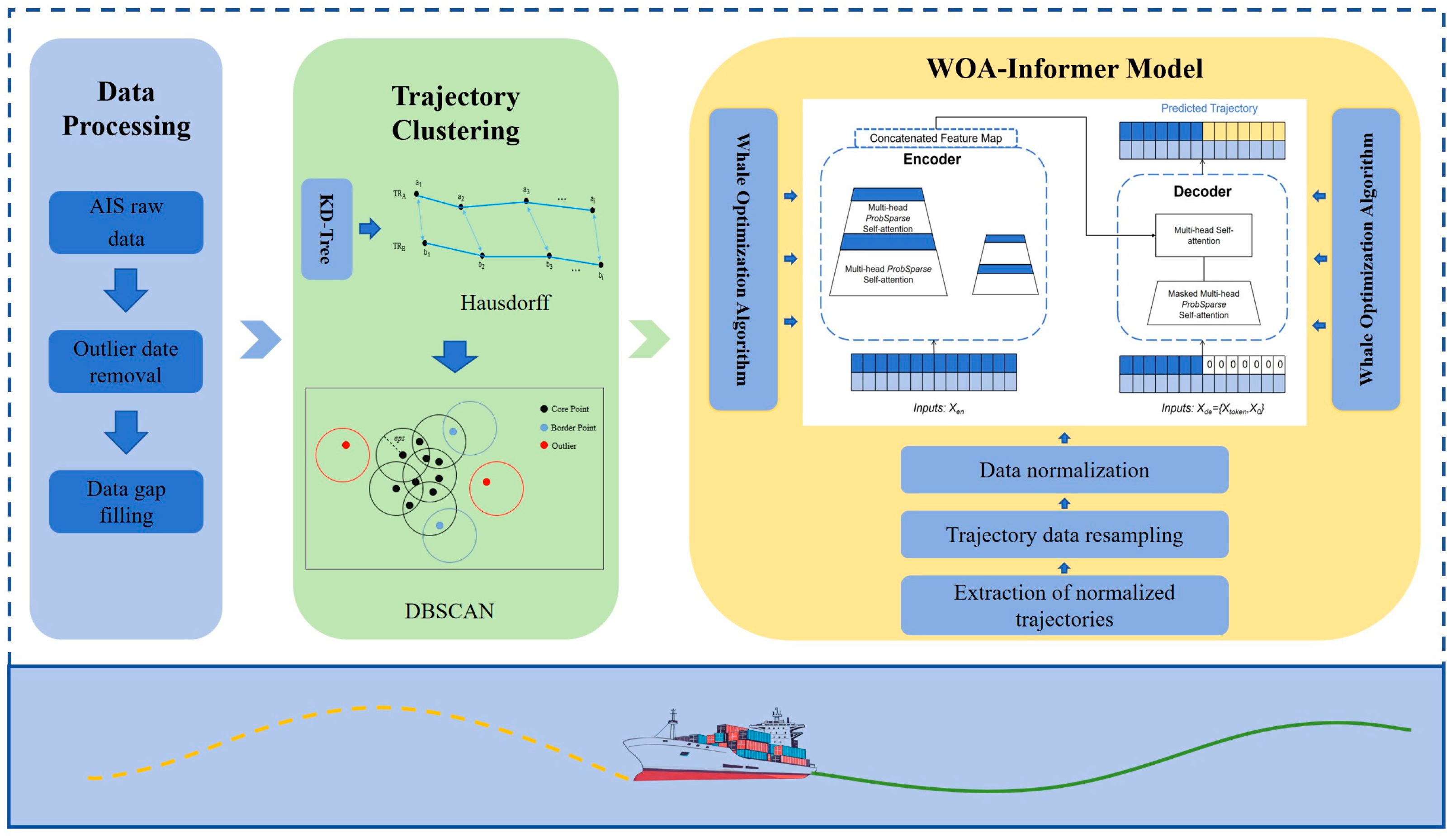
Figure 1. Overall model design flow chart.
Jmse 13 01999 g001
Figure 2. WOA optimization process.
Jmse 13 01999 g002
Figure 3. DBSCAN clustering schematic.
Jmse 13 01999 g003
Figure 4. Diagram of Hausdorff distance.
Jmse 13 01999 g004
Figure 5. KD-Tree algorithm flow chart.
Jmse 13 01999 g005
Figure 6. Informer model architecture.
Jmse 13 01999 g006
Figure 7. WOA flow chart.
Jmse 13 01999 g007
Figure 8. The visualization of trajectory data within the study region. (a) Raw trajectory dataset. (b) Raw trajectory dataset details. (c) Post-processed trajectory data. (d) Post-processed trajectory dataset details.
Jmse 13 01999 g008
Figure 9. Visualization of trajectory clustering.
Jmse 13 01999 g009
Figure 10. Execution time distribution.
Jmse 13 01999 g010
Figure 11. Trajectory pattern. (a) Case 1. (b) Case 2. (c) Case 3.
Jmse 13 01999 g011aJmse 13 01999 g011b
Figure 12. Prediction results of trajectory pattern 1. (a) Overall trajectory diagram. (b) Partial trajectory diagram.
Jmse 13 01999 g012
Figure 13. Prediction results of trajectory pattern 2. (a) Overall trajectory diagram. (b) Partial trajectory diagram.
Jmse 13 01999 g013
Figure 14. Prediction results of trajectory pattern 3. (a) Overall trajectory diagram. (b) Partial trajectory diagram.
Jmse 13 01999 g014
Figure 15. Performance comparison of trajectory pattern 1.
Jmse 13 01999 g015
Figure 16. Performance comparison of trajectory pattern 2.
Jmse 13 01999 g016
Figure 17. Performance comparison of trajectory pattern 3.
Jmse 13 01999 g017
Table 1. Experimental environment configuration.
EnvironmentSpecific Configuration
Operating SystemWindows 11
CPUi5-12450H
GPURTX 3060
Programming LanguagePython 3.11.7
CompilerPyCharm 2021
FrameworkPyTorch 2.5.1
Table 2. Partial ship AIS data.
MMSIBase Date TimeLAT (°)LON (°)SOG (kn)COG (°)
3529861462024-11-08T10:39:3636.02465120.339088.9281.6
3529861462024-11-08T10:41:0536.02541120.334569.0281.5
3529861462024-11-08T10:43:3436.02672120.3265910.1281.3
3529861462024-11-08T10:45:0736.02763120.3212710.8281.8
3529861462024-11-08T10:46:3436.02864120.3156211.4282.1
Table 3. The hyperparameters to be optimized.
HyperparametersSet RangeStep Size
Learning rate[0.0001, 0.1]0.0001
Batch size[2, 128]1
Encoder layers[1, 6]1
Decoder layers[1, 6]1
Dropout[0.005, 0.4]0.01
Table 4. Optimized result.
HyperparametersCase 1. ResultCase 2. ResultCase 3. Result
Learning rate0.00470.00360.0023
Batch size382923
Encoder layers223
Decoder layers122
Dropout0.130.190.24
Table 5. Hyperparameter settings.
ModelHyperparameterHyperparameter Set
CNN-BILSTMFilter size
Regularization
Activation function
Attention type
4
L2
Relu/Sigmoid
None
TransformerEncoder–Decoder Layers
Head number
Activation function
Attention type
[2, 1]
8
Gelu
Self-attention
InformerEncoder–Decoder Layers
Head number
Activation function
Attention type
[2, 1]
8
Gelu
ProbSparse attention
Table 6. Evaluation metrics for trajectory pattern 1 prediction results.
ModelRMSE (10−3)MAE (10−3)MAPE (10−3)HAV (m)
CNN-BILSTM0.9270.6780.692107.7
Transformer0.5630.4350.52266.90
Informer0.4470.3030.38450.24
WOA-Informer0.3420.2880.46243.21
Table 7. Evaluation metrics for trajectory pattern 2 prediction results.
ModelRMSE (10−3)MAE (10−3)MAPE (10−3)HAV (m)
CNN-BILSTM1.5541.1051.352168.23
Transformer0.7210.5670.89791.95
Informer0.7510.5650.92295.77
WOA-Informer0.6460.4310.52769.19
Table 8. Evaluation metrics for trajectory pattern 3 prediction results.
ModelRMSE (10−3)MAE (10−3)MAPE (10−3)HAV (m)
CNN-BILSTM1.6261.1511.604189.64
Transformer1.2880.8450.986137.81
Informer1.2340.7280.794122.67
WOA-Informer0.8410.5200.68782.87
Table 9. Model Execution Time.
ModelPattern 1 Execution Time (s)Pattern 2 Execution Time (s)Pattern 3 Execution Time (s)
CNN-BILSTM52.45747.65158.658
Transformer27.18624.25632.156
Informer18.26917.14720.015
WOA-Informer22.13219.89325.867
Disclaimer/Publisher’s Note: The statements, opinions and data contained in all publications are solely those of the individual author(s) and contributor(s) and not of MDPI and/or the editor(s). MDPI and/or the editor(s) disclaim responsibility for any injury to people or property resulting from any ideas, methods, instructions or products referred to in the content.