Article

Online Sparse Sensor Placement with Mobility Constraints for Pollution Plume Reconstruction

1
College of Environmental and Resource Sciences, Zhejiang University, Hangzhou 310058, China
2
College of Engineering, Westlake University, Hangzhou 310030, China
*
Author to whom correspondence should be addressed.
J. Mar. Sci. Eng. 2025, 13(10), 1995; https://doi.org/10.3390/jmse13101995
Submission received: 22 September 2025 / Revised: 11 October 2025 / Accepted: 15 October 2025 / Published: 17 October 2025
(This article belongs to the Section Ocean Engineering)

Abstract

The rational placement of pollutant monitoring sensors has long been a prominent research focus in ocean environment science. Our method integrates an incremental Proper Orthogonal Decomposition with a mobility-constrained sensor selection strategy, enabling efficient monitoring and dynamic adaptation to spatio-temporal field changes. At each time step, the position of the sensors is updated based on the incoming measurements to minimize the reconstruction error while adhering to movement constraints. This online approach considers the need for mobility distance, making it suitable for long-term deployments in resource-limited scenarios. The proposed framework is validated in three scenarios: a linear advection–diffusion system with multiple moving pollution sources, the distribution of particulate matter with an aerodynamic diameter smaller than 2.5 μm (PM2.5) across the United States, and scalar transport in flows past side-by-side cylinder arrays in the ocean. The results demonstrate that the method achieves high reconstruction accuracy with significantly fewer sensors. This study conducts a comparative analysis of three typical mobility constraints and their respective effects on reconstruction accuracy. In addition, the proposed localized sensor mobility strategy effectively tracks evolving plume structures and maintains a low approximation error, providing a generalizable solution for sparse monitoring of the marine environment.

1. Introduction

Environmental observation with scarce data has long been a challenging issue [1], particularly in expansive and dynamic environments such as oceanic [2,3], lacustrine [4,5], and wildfire-affected regions [6,7]. Previous studies have focused on domain-specific modeling and remote sensing techniques to capture pollutant transport or ecosystem dynamics within environments. However, most of these approaches rely on dense or static sensor networks, making them impractical for large-scale or mobile monitoring scenarios. This gap motivates the development of adaptive, data-efficient methods capable of reconstructing spatiotemporal environmental fields under mobility and sparsity constraints. A well-designed sensor observation placement and wireless sensor networks [8] hold promise for addressing this issue. The accurate reconstruction of spatiotemporal information of pollutants within a limited number of sensors has remained a highly active research topic for decades [9,10,11,12,13]. By deploying autonomous buoy robots [14], local surface information on temperature, salinity, and dissolved oxygen can be effectively acquired. The deployment of a systematic buoy array [15] can significantly improve the monitoring and early warning capabilities for marine environmental conditions. However, how to update their positions online at the planning level, and whether point-by-point mobile measurements are required to reconstruct large-scale ocean information, remains insufficiently explored.
Sensor placement indicates areas of high sensitivity in environmental monitoring. The problem is typically decomposed into two fundamental components: How can the optimal dynamic sensor placement with limited mobility be obtained? How accurately can the environmental field be reconstructed based on limited measurements? In this work, our study addresses this question through a linearized theory representation.
The sensor placement problem is essentially an NP-hard combinatorial optimization challenge. Given candidate grid points n, the task of selecting sensor locations p leads to a combinatorial search space of size n p = n ! p ! ( n p ) ! , which grows exponentially with both n and p. As a result, an exhaustive search becomes computationally intractable, even for moderately sized problems. Traditional global optimization techniques are often impractical in real-time or large-scale applications because of their high computational cost. In the field of sensor placement optimization, researchers have explored a variety of approaches, including reduced modeling [16], data-driven active learning [17], and heuristic optimization strategies [18]. Manohar et al. [19] adopts a balanced feedback strategy to select sensors according to the norm H 2 and H , compared to the traditional greedy QR selection [20]. Zhang et al. [21] suggests a selection and reconstruction method based on the entropy-maximization policy. Marcato et al. [22] presents a differentiable plan for training a sensor trajectory by a transformer model to obtain the gradient to optimize sensor positions in the next step. Gao et al. [23] introduces a generative model to generate a placement representation in city environment monitoring by learning from a large amount of data. Andersson et al. [24] develops a ConvGP model by selecting a set of high-uncertainty sensor points in the pretrained network. Advanced dynamic mode decomposition (mrDMD) methods can leverage simulation data to optimize sensor placement, with the primary objective of constructing an optimal observation matrix [25,26].
Although the aforementioned methods are capable of selecting informative observation points, all of them rely heavily on large-scale pre-training data and lack a truly incremental learning process. In practical scenarios, sequentially acquiring data over time is regarded as a form of online learning. To improve monitoring efficiency and reconstruction accuracy without increasing hardware costs, this study suggests a framework of linear theory, inspired by incremental learning [27,28] and Proper Orthogonal Decomposition [29,30]. It is essential to clarify that this work primarily employs a linear decomposition theory to address the aforementioned problems. In contrast, non-linear approaches typically rely on data-driven training, which is inherently data-hungry and requires a large amount of high-quality training data, posing a significant challenge in the application. The goal is to adaptively update the placement of a fixed number of sensors over time, thereby progressively improving both observation efficiency and reconstruction accuracy. Our approach consistently outperforms traditional selection strategies by providing near-optimal sensor configurations under mobility constraints.
The remainder of this article is organized as follows. Section 2 presents the underlying principles of the proposed method and describes the composition of the data set and associated tasks. Section 3 demonstrates the performance of the method in three problems. Finally, Section 4 provides a detailed analysis and discussion of the proposed approach.

2. Methodology

In this section, we will introduce our methods, dataset, and evaluation metric details.

2.1. Overall Framework and Principle

The framework is illustrated in Figure 1. The method takes the pollutant concentration field at every time step as input and outputs the corresponding optimal sensor placement. Given an incremental sequence of snapshots X k , the algorithm incrementally updates the subspace U k and outputs sensor locations adaptively over time. The details of implementing sensor placement are provided in Section 2.2 and Section 2.3.

2.2. Incremental POD and QR Sensor Selection

This paper employs an incremental Proper Orthogonal Decomposition (POD) algorithm [31] to adaptively update the basis and apply QR pivoting [32] to select sensor locations that preserve observability while minimizing reconstruction error. POD is based on linear theory, where the state of the system at time t is denoted by x ( t ) R n .
Given a set of snapshots collected at discrete steps, the snapshot matrix X k at step k is
X k = [ x 1 ,   x 2 ,   ,   x k ] R n × k .
At each time step k, an orthonormal basis U k 1 R n × r is constructed from previous snapshots. When a new snapshot x k arrives, the residual r k is computed in the current subspace:
r k = x k U k 1 U k 1 x k .
If the residual satisfies r k > ε , it is normalized and appended to the following basis:
U k = [ U k 1 , r k r k ] .
Once the updated basis U k is obtained, we select the locations of the sensors p that preserve the subspace structure. This is achieved via column-pivoted QR decomposition:
U k = Q R P ,
where P is a permutation matrix. The indices corresponding to the first p rows in P define the sensor locations. C k R p × n denote the observation matrix that extracts the selected x k . The corresponding measurements are
y k = C k x k .
The full state is used as a least-squares projection onto the learned subspace U k .
x k U k a k , a k R r .
Since only a subset of the state is observable through the matrix C k , the measurement at time k is given by
y k = C k x k C k U k a k .
To estimate the coefficient vector a k , we solve the following least-squares problem:
a k = arg min a C k U k a y k 2 2 .
The solution is obtained via the Moore–Penrose pseudoinverse:
a k = ( C k U k ) y k .
The reconstructed state x ^ k is the full state by mapping back to the high-dimensional space:
x ^ k = U k a k = U k ( C k U k ) y k .
This procedure enables the reconstruction of the high-dimensional system state from a small number of sparse measurements, under the assumption that the system dynamics is predominantly captured by the low-dimensional basis U k .

2.3. Local QR-Based Sensor Selection with Mobility Constraints

The local QR algorithm is initialized using the selected sensor locations based on the global QR method in the first step of this study. Although the global QR initialization determines the initial sensor layout, its influence diminishes as the local QR selection progressively updates the sensor positions based on new field information, thereby maintaining adaptability and long-term robustness against initial placement bias. This setting is consistent with practical monitoring scenarios, where the initial estimation of the field may come from satellite observations or numerical models. In such cases, a reliable initial layout is essential for guiding sensor mobility in the early stages of adaptation. However, the initial sensor locations could be randomly selected or manually specified. To add mobility constraints to the sensor, we introduce a local adaptive QR-based selection strategy. Let S k { 1   , 2 ,   ,   n } denote the sensor locations selected at time step k. The constraints enforce three practical requirements:
  • The sensor number constraint: | S k | = p ensures that the locations of the sensors are selected exactly p.
  • Mobility constraint: Each new sensor location s j ( k ) must be within a local neighborhood (with distance J max ) of a previous location s j ( k 1 ) , limiting how far a sensor can move between time steps.
  • Minimum Separation Constraint: All selected sensor pairs ( s i ( k ) ,   s j ( k ) ) must be at least d min distance apart to avoid spatial redundancy and ensure spatial diversity in observations.
This local QR ensures that each sensor only follows and moves within a restricted distance, making the method applicable to mobile sensing systems with both mobility and spatial separation constraints. The optimization problem in each time step k is formulated as
min S k { 1 , , n } x k U k a ( S k ) 2 x k 2 subject to 1 . | S k | = p , 2 . a ( S k ) = arg min a R r x k [ S k ] U k [ S k , : ] a 2 , 3 . s j ( k ) S k , s j ( k 1 ) S k 1 such that s j ( k ) s j ( k 1 ) J max , s i ( k ) s j ( k ) d min , i j .
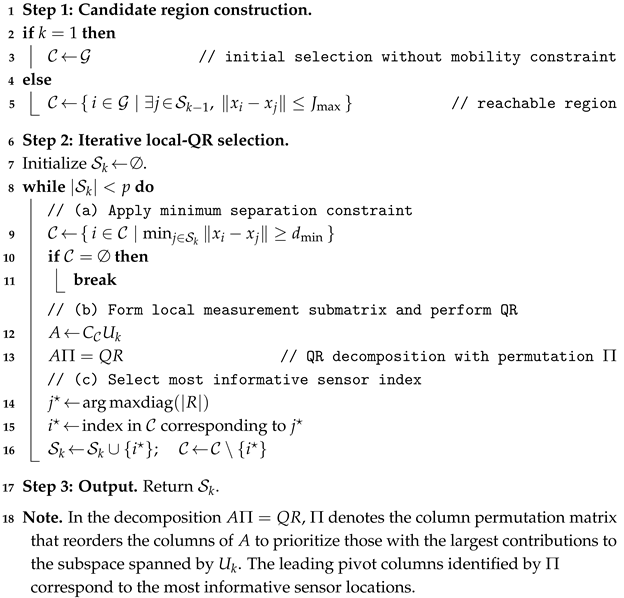
To solve this problem, possible candidate locations are generated within a search radius, a QR decomposition of the local POD basis prioritizes informative points, and the final selection is enforced to satisfy both mobility and separation constraints. The algorithm as shown in Algorithm 1 in this study is deterministic, and repeated runs under identical settings produce identical results.
Algorithm 1: Local QR-based Sensor Selection with Mobility and Separation Constraints
Input: POD basis U k R n × r at time step k; previous sensor set S k 1 ;candidate grid 𝒢 = { 1 ,   ,   n } with coordinates { x i } ;number of sensors p; mobility limit J max ; minimum separation d min .
Output: Selected sensor set S k with | S k | = p .
Jmse 13 01995 i001

2.4. Datasets Description

To validate the generality of the proposed method across analytical, real-world, and simulated flow environments, three representative datasets were employed. These datasets were selected to cover both idealized and realistic pollution transport scenarios relevant to maritime and atmospheric monitoring. In each case, we emphasize how the data represent practical sensor-network conditions, including limitations in sensor density, communication, and energy availability. The PM2.5 dataset represents a realistic large-scale monitoring scenario with sparse sensors, analogous to maritime or coastal pollution observation networks. Each virtual sensor can be viewed as a stationary or slowly mobile buoy or ground-based measurement unit, where communication and energy constraints limit spatial density. This dataset therefore provides a real-world context to test the scalability and sparsity-robustness of the proposed framework. This analytical case provides a controllable benchmark to evaluate reconstruction accuracy under known physical conditions. It mimics an idealized pollution release in a small marine or estuarine region, where advection and diffusion dominate pollutant transport. Such a scenario reflects situations in which sensor coverage is limited by marine energy supply or deployment constraints, enabling a clear evaluation of sensor mobility effects. The final case extends the analysis to a canonical fluid–structure interaction system that captures pollutant dispersion in complex wake flows—an analog to local pollutant mixing around offshore platforms or ship hulls. It allows for evaluating whether the proposed sensor selection method can adapt to strong unsteady vortical structures and constrained sensor mobility. The simulation setup also provides insight into how physical constraints affect reconstruction accuracy.

2.4.1. An Analytical Solution with Three Point Sources

Considering an ideal but representative linear-advection–diffusion equation [33,34],
u t + a u x + b u y = ν 2 u x 2 + 2 u y 2 , ( x , y ) R 2 , t > 0 ,
where u ( x , y , t ) denotes the transported scalar, a and b are constant convection velocities in the x and y directions, respectively, and ν > 0 is the diffusion coefficient, in the case of multiple-point sources located at ( x j , y j ) with strengths c j . For the unbounded plane R 2 , the fundamental solution of the advection–diffusion Equation (12) is the following fundamental solution:
u ( x , y , t ) = j = 1 N c j 4 π ν t exp ( x x j a t ) 2 + ( y y j b t ) 2 4 ν t , t > 0 ,
where the term ( x j , y j ) represents the position of the source, while the linear drift is ( a t , b t ) .
In this case, we define a uniform background flow with velocity components a = 0.1 m s 1 and b = 0.1 m s 1 , as shown in Figure 2. The spatial observation domain is set to [ 10 m , 10 m ] 2 . The diffusion coefficient is chosen as ν = 0.01 m 2 s 1 . Three-point sources are at the positions ( x 1 ,   y 1 ) = ( 0 m ,   0 m ) , ( x 2 ,   y 2 ) = ( 5 m ,   5 m ) , and ( x 3 ,   y 3 ) = ( 0 m ,   6 m ) , each source with a uniform strength of c j = 0.1 kg . Observations are recorded from t = 1 s to t = 61 s at regular intervals of Δ t = 10 s .

2.4.2. A Case Study on PM2.5 Emission in the United States

This study used a publicly available monthly PM2.5 model for the United States in 2016 [35]. Applying a uniform sparse sampling with a stride of 50, we transformed the original dataset into measurements of 3328 sensors in the spatial space, as shown in Figure 3.

2.4.3. A Case Study on Side by Side Cylinders

The governing equations are as follows. The flow field is described by the incompressible Navier–Stokes equations,
t u + u · u = p + R e 1 2 u , · u = 0 ,
where u is the velocity field, p the pressure, and R e the Reynolds number. The scalar field is governed by the advection–diffusion equation,
t c + u · c = ( R e S c ) 1 2 c , ( x ,   y ) [ 0 , L x ] × [ 0 , L y ] ,
where c denotes the passive scalar concentration and S c is the Schmidt number. The right-hand side ( R e S c ) 1 reflects the effects of momentum and scalar diffusion.
In this study, we consider a relatively complex scalar transportation within S c = 1 , R e = 100 , using a side-by-side cylinder layout, as shown in Figure 4. The uniformly distributed line source, indicated by the yellow line in the figure, is incorporated into the simulation, where the fluid state is resolved with the WaterLily solver [36]. The computed fluid state is substituted into the convection–diffusion equation to obtain the pollution concentration C ( x ,   y ,   t ) . At the post-processing stage, a finite-difference post-processing step is applied to the concentration field to ensure mass conservation. The fluid simulation was conducted with a time step of 0.1 t U / D , where U = 1 denotes the uniform inflow velocity and D is the diameter of the cylinder. The center-to-center spacing between the two cylinders was set to 2 D . A uniform grid of 514 × 514 was employed, with no sensors placed inside the cylinders. The total number of sensors was 262,572. As shown in Figure 4D, the integrated mass of the concentration field remained constant at 1, indicating that the finite-difference scheme preserves mass conservation.

2.5. Evaluation Metric

Throughout the following experiments, the residual tolerance ϵ is defined as 1 × 10 6 , which is the empirical value. In this study, under varying constraints on the setting, we consider the following questions: (1) How does the number of sensors p affect the reconstruction? (2) How do mobility limits J m a x influence reconstruction? (3) How could mini-separation d m i n influence the results? Relative error is used as the performance metric.
Rel Error = X ^ X 2 X 2 ,
where X ^ is the reconstructed value and X is the true value.
To further quantify sensor mobility, this study reports two statistical values: (1) The average movement length L ¯ ; (2) The maximum movement length L max . Let s j k be the position of the sensor j at time step k.
L ¯ = 1 ( T 1 ) p k = 1 T 1 j = 1 p s j ( k + 1 ) s j ( k ) 2 , L max = max k , j s j ( k + 1 ) s j ( k ) 2 .
At time step k, the observation matrix is A k : = C S k U k R p × r , where U k is the POD basis and C S k samples rows at the selected sensor set S k . We quantify numerical stability by the condition number
κ ( A k ) = σ max ( A k ) σ min ( A k ) ,
where σ max and σ min are the largest and smallest singular values of A k . If σ min ( A k ) = 0 (rank deficient), κ ( A k ) = . Smaller κ ( A k ) implies better numerical stability and more reliable field reconstruction, while large κ ( A k ) indicates noise amplification and unstable inversions.

3. Experiments and Discussion

3.1. The Performance of Case1

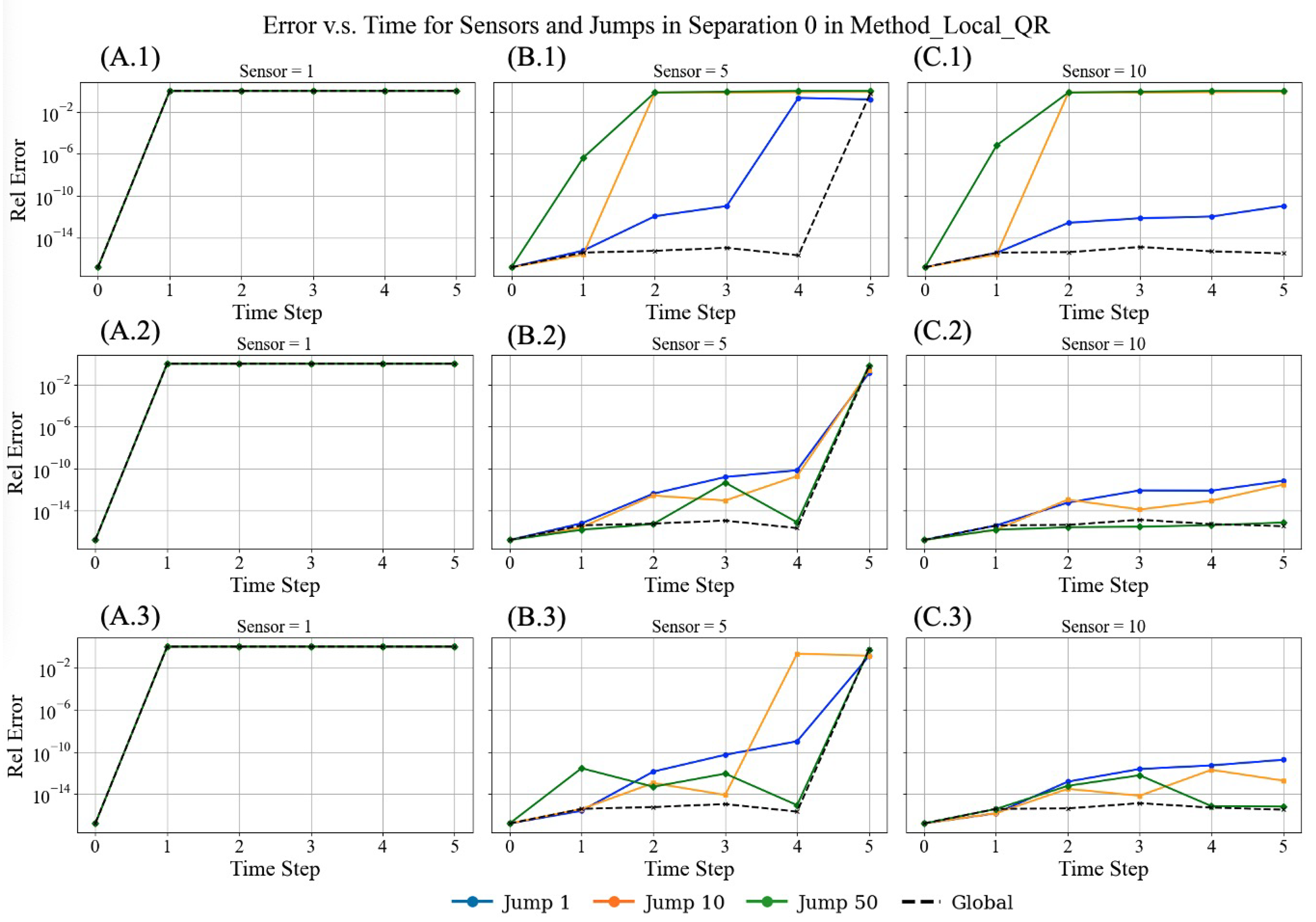
To quantitatively evaluate and compare the reconstruction performance of local QR and global QR methods within the incremental POD framework, we conducted experiments under a range of mobility constraints. Specifically, we tested three conditions for the maximum sensor displacement, ( J max 1 ,   10 ,   50 measured in grid units), along with varying the number of sensors ( p 1 ,   5 ,   10 ) and the minimum separation distances ( d min 0 ,   1 ,   10 grid units). The results of these comparative experiments are summarized in Figure 5, Figure 6, Figure 7, Figure 8 and Figure 9. These figures collectively illustrate how the reconstruction accuracy and sensor trajectories vary with the number of sensors, jump limits, and separation distances. In particular, Figure 5 compares local and global QR strategies, while Figure 6, Figure 7 and Figure 8 visualize how sensor paths adapt to plume advection, revealing that reconstruction effect and mobility constraints significantly affect both reconstruction stability and sensor clustering.
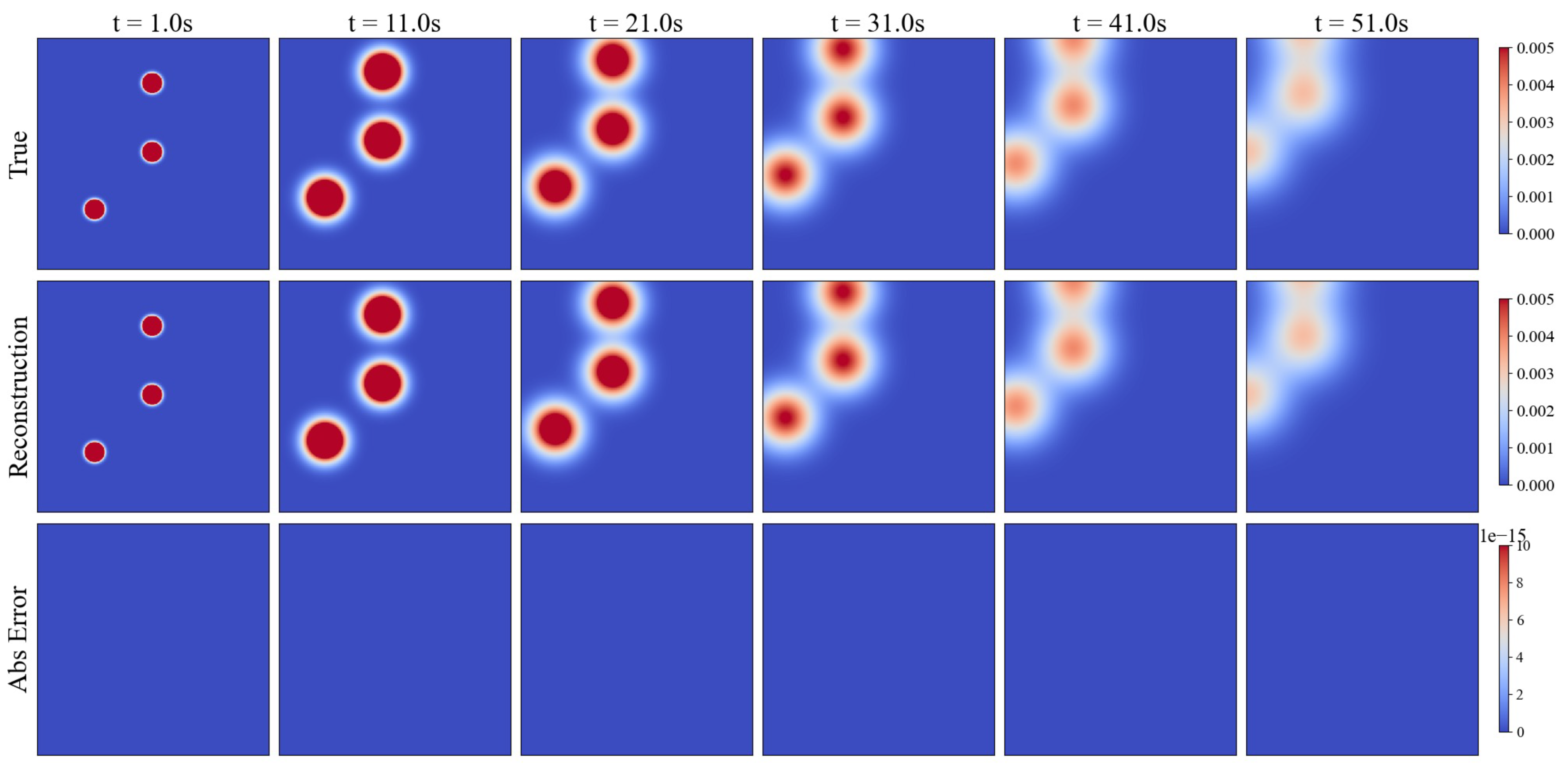
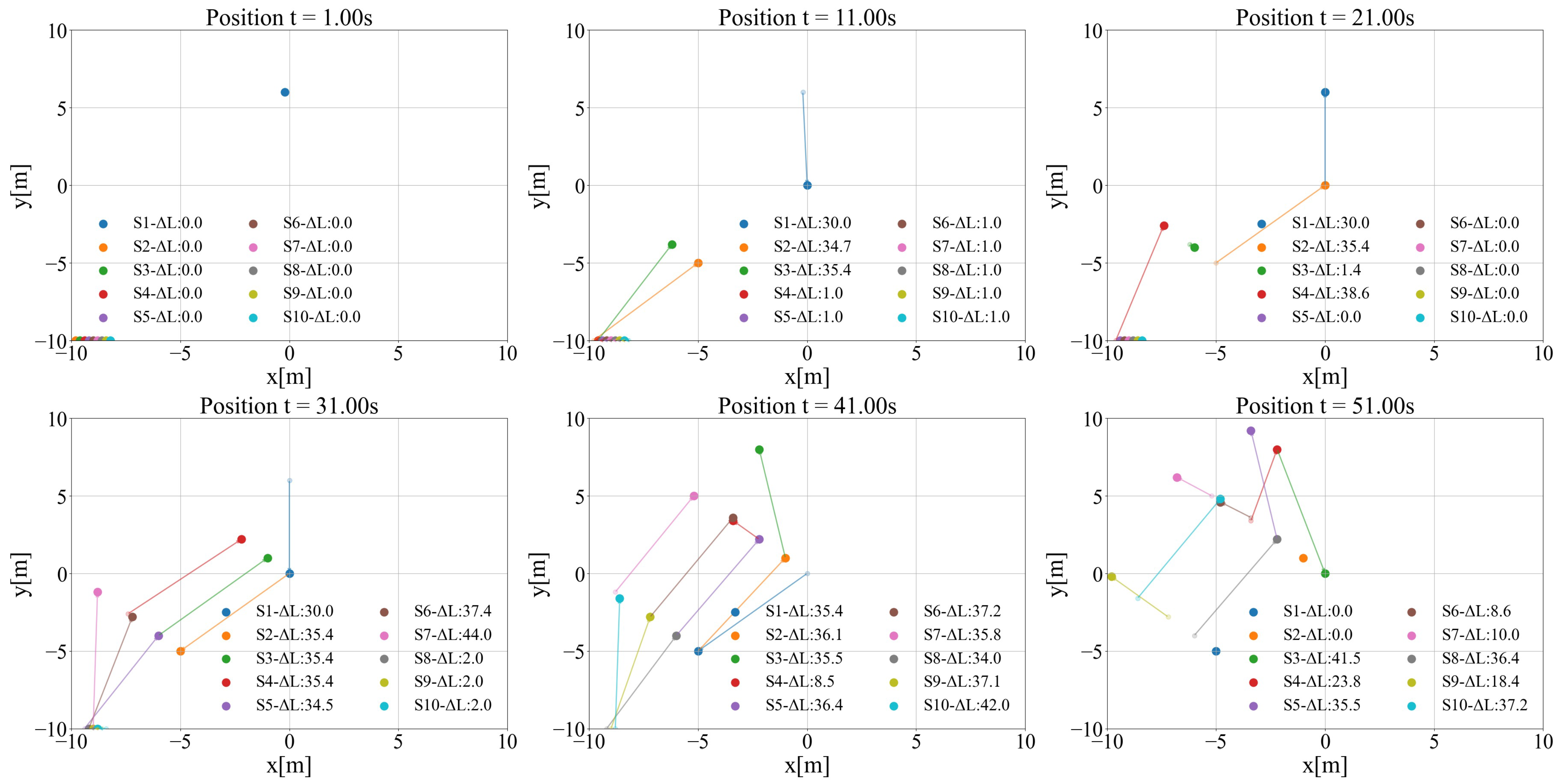
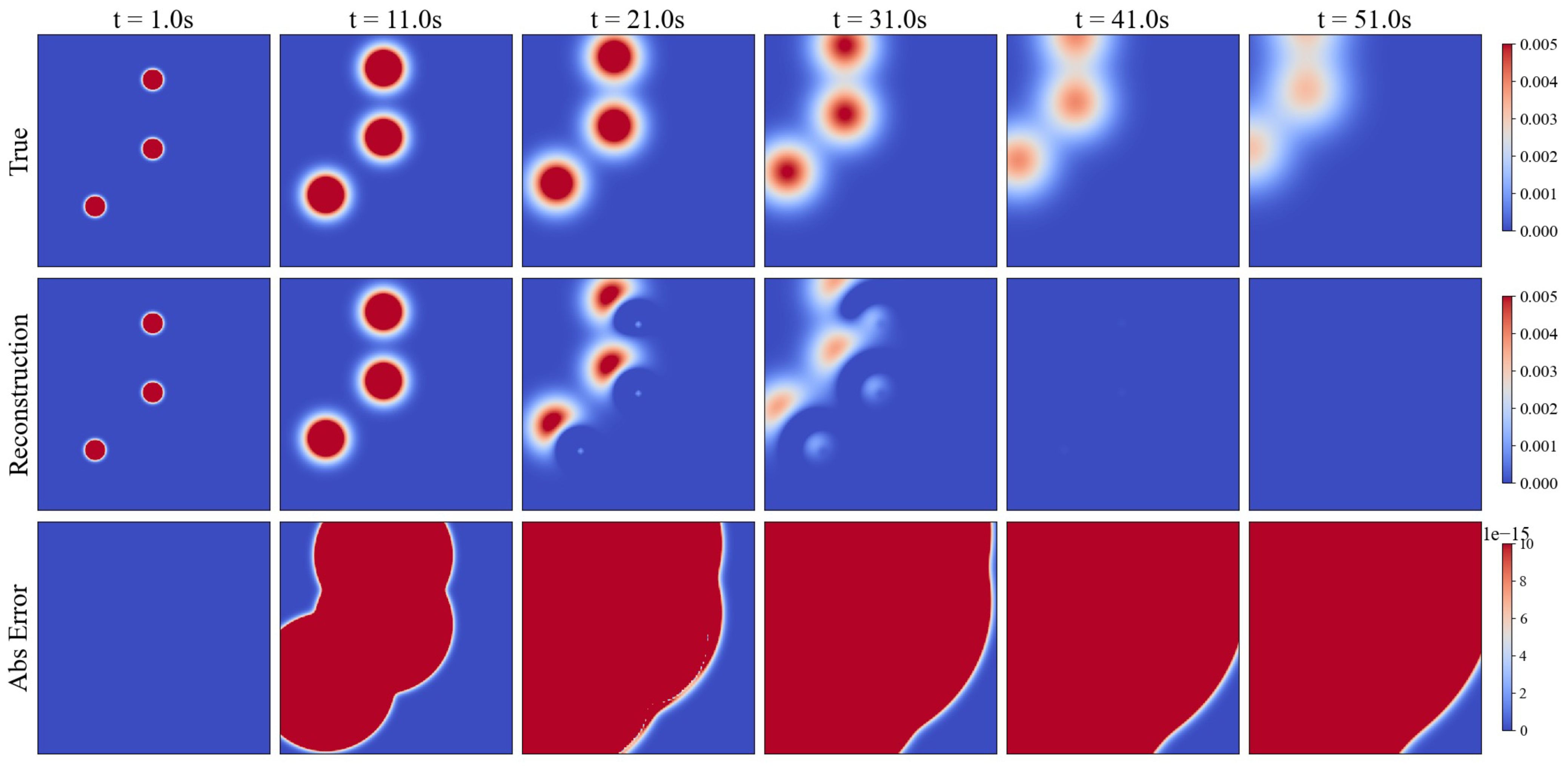
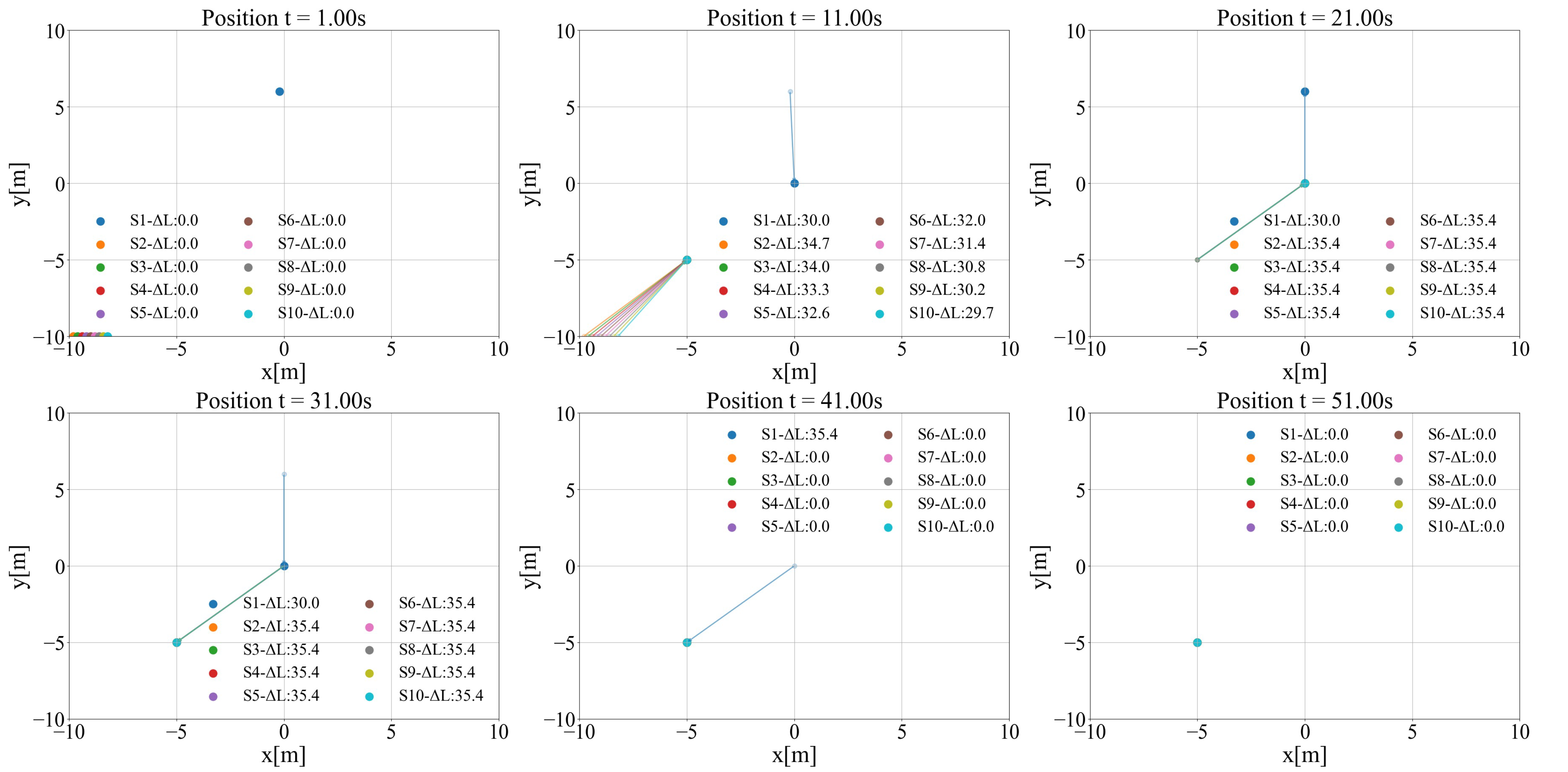
Increasing the number of sensors p from one to ten significantly improves the accuracy of the reconstruction in the local QR and global QR methods. For example, with only one sensor p = 1 , regardless of the local or global QR, there are steep errors after the first step, indicating the inherent limitation of measurements in capturing system dynamics. In contrast, with ten sensors( p = 10 ), the global QR consistently achieves a low error, while the local QR performance becomes less competitive because the movement distance is relatively short. As shown in Figure 6 and Figure 7, the sensor positions adjust dynamically with time, following the drift of the pollutant plume, which moves toward the upper left direction. Since only the first three modes can effectively capture the dominant dynamics, the system requires only three sensor movements at t = 41 s and t = 51 s to sufficiently track the underlying information.
Within each subplot in Figure 5, the solid lines represent local QR with varying mobility constraints. A consistent trend can be observed: smaller jump limits (e.g., J m a x = 1 ) generally result in lower reconstruction errors, particularly in the early time steps. This suggests that frequent but localized sensor updates are more effective than infrequent long-distance repositioning. For example, in Figure 5(B.1,C.1), the J m a x = 1 within d m i n = 0 strategy outperforms J m a x = 10 and J m a x = 50 . The reason for this is that larger jump distances make the sensors greedily converge to the same location, as shown in Figure 10, leading to fewer observations.
Comparison between rows reveals that larger minimum separation distances (e.g., d m i n = 10) degrade local QR performance, especially when combined with fewer sensors. This is likely due to reduced spatial diversity in the placement of the sensor, which limits the information available for reconstruction. In particular, this degradation is most evident in Figure 5(B.3,C.3), where high separation and low sensor counts lead to increased error. Appropriate separation can prevent redundancy, but if the distance d m i n is too large, it will still reduce flexibility and make it difficult for the algorithm to select key areas adaptively.
Fundamentally, the global QR is designed to maintain the numerical stability of the observation matrix C k U k by preserving the orthogonality of the matrix basis. However, the local QR is reconstruction-oriented: it prioritizes selecting sensor locations that yield accurate field recovery using a small number of sensors p, even if this leads to a higher condition number in Table 1. In terms of sensor mobility, the global QR method exhibits the smallest average movement distance of 14.96; its maximum movement distance is significantly larger than the other two methods, reaching 84.74. For the two local QR configurations with a maximum jump limit of J = 50 , the average movement distances under d min = 0 and d min = 1 are nearly identical. However, setting with d min = 0 results in extremely large condition numbers like inf, even reaching infinity in certain time steps, which is detrimental to reconstruction performance. This highlights the importance of incorporating a minimum separation constraint d m i n to balance sensor mobility with numerical stability in reconstruction tasks.

3.2. The Performance of Case2

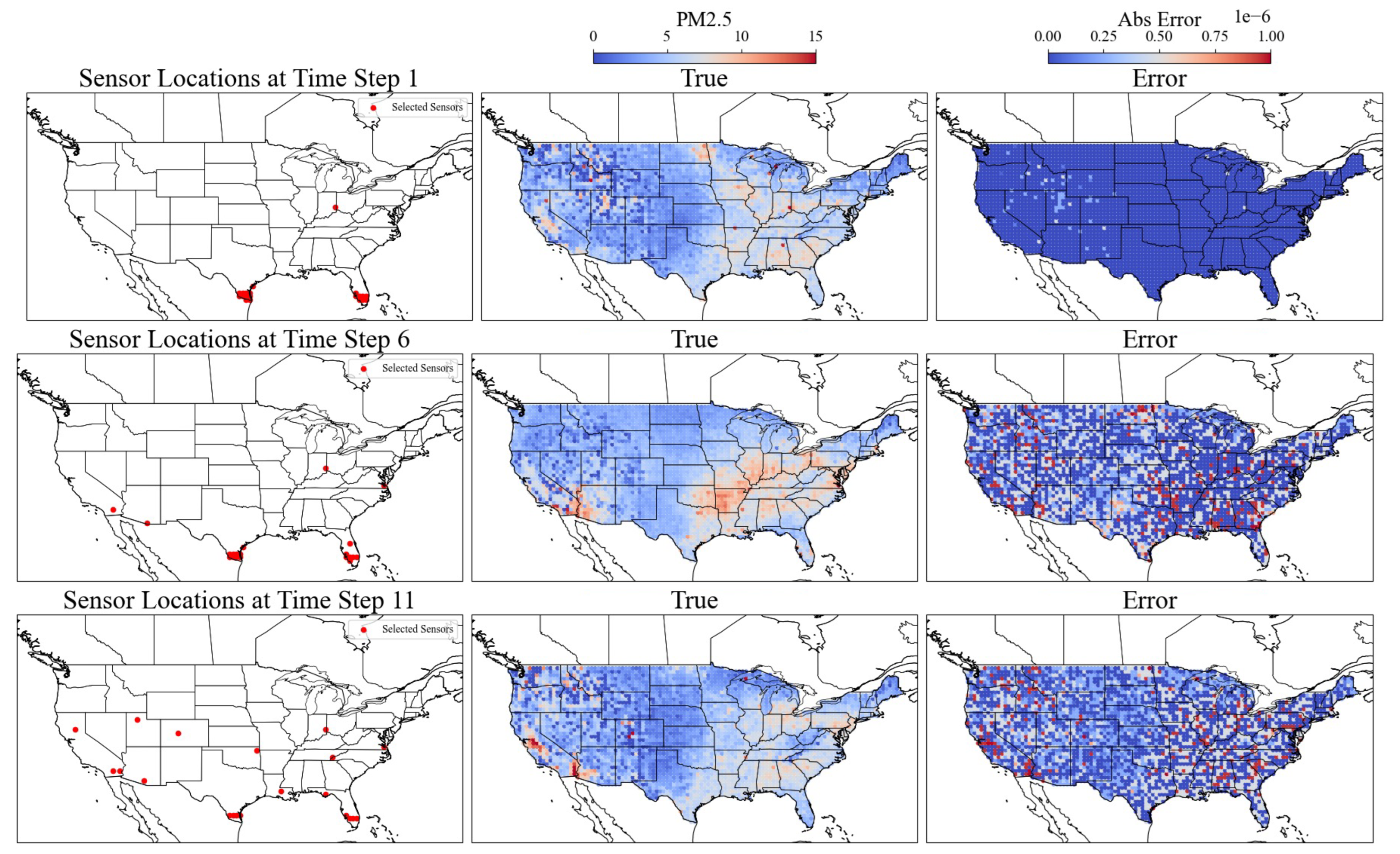
Similarly to case 1, we performed experiments for this case using a wider range of sensor counts, specifically comparing configurations with 1, 5, 10, and 20 sensors. In this experiment, we used the actual geodesic distance on the Earth’s surface (in kilometers) to constrain the sensor movement range at each time step. Specifically, the maximum jump distances J m a x are set to 1, 50, and 500 km, while the separation constraints d m i m between the sensors are set to 0, 50, and 100 km, respectively. Figure 11, Figure 12 and Figure 13 visualize the differences in reconstruction behavior between the global QR and local QR approaches. The condition numbers of the sensor metrics are summarized in Table 2. The global QR strategy exhibits the largest single-step jump ( L max = 3313.5 km) and the mean displacement ( L ¯ = 395.4 km), meaning that a sensor may need to travel a long distance in a short time, placing demanding requirements on the mobile sensor. When a 500 km mobility constraint is enforced with d min = 10 , performance improves markedly: l max drops to 493 km and the reconstruction matrix retains the lowest condition number. By contrast, with d min = 0 , a greedy effect drives the condition number to infinity. Even though the mean displacement is only 102.8 km, the large condition number prevents accurate recovery from t 3 , and all subsequent reconstructions deteriorate.
The limitations of larger jumps with smaller sensors may cause the algorithm to miss informative regions, leading to error spikes. When using a large constraint (e.g., J m a x = 50 in Figure 11(B.1,C.1,D.1)), the impact of the sensor quantity becomes critical. With only ten sensors, the reconstruction process is susceptible to any suboptimal placement, as each sensor carries substantial weight in the projection matrix. This makes the method prone to instability when a few sensors jump to low-information regions. In contrast, with 20 sensors, the increased spatial redundancy provides robustness. The improvement is primarily due to its improved capacity to capture the dominant modes of the system. The resulting sensing matrix better preserves orthogonality and conditioning, leading to more stable and accurate reconstructions in Figure 11(C.2,D.2). The relative results are shown in Figure 12 and Figure 13.

3.3. The Performance of Case3

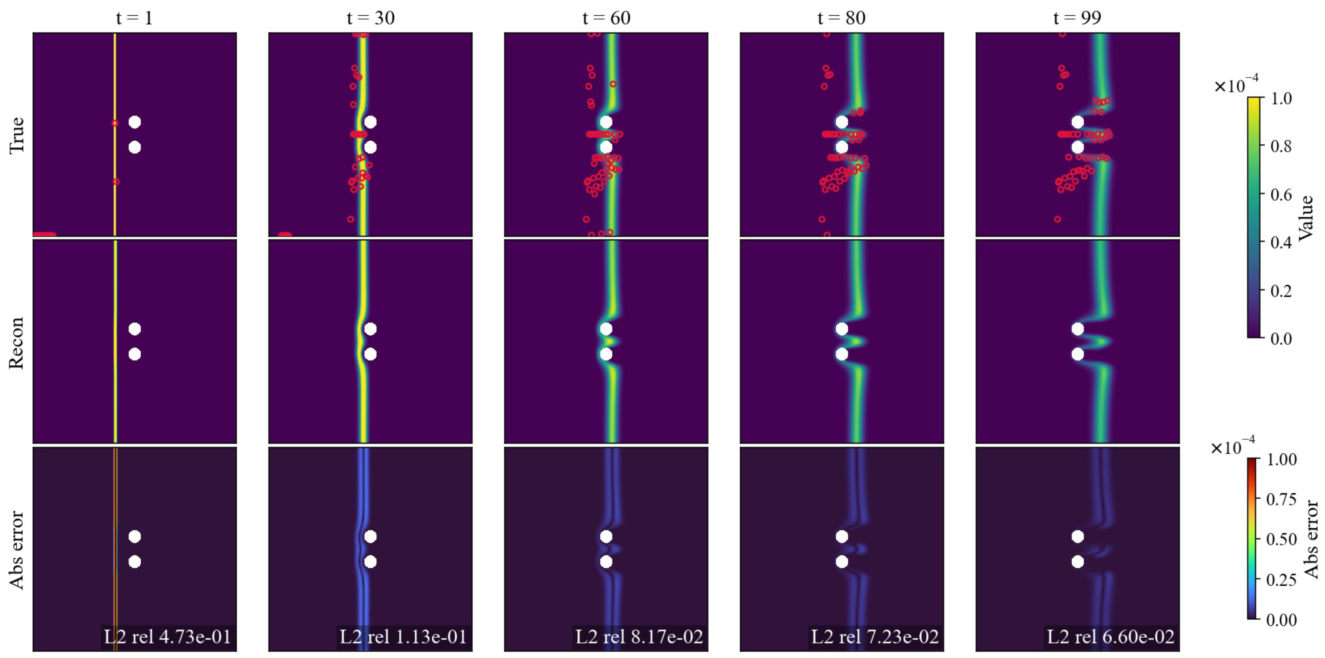
In the evaluation, the number of sensors was chosen as p { 1 , 10 , 50 } . The maximum jump distance was set as J max { 10 , 100 , 1000 } grid units, and the minimum separation constraint was selected as d m i n { 0 , 10 , 100 } grid units. The results of Case 3 are presented in Figure 14. The two extreme cases, corresponding to the best and worst results, are illustrated in Figure 15 and Figure 16. The mobility statistical results are summarized in Table 3. Since case 3 involves a large number of time steps, we do not present the variations in condition number over time.
In the case of a single sensor in Figure 14A, the error remains nearly constant across all configurations, indicating that performance is limited by insufficient information rather than constraint settings. With ten sensors in Figure 14B, the error becomes more sensitive to the minimum separation d min and the maximum jump J max . A large separation with a small jump radius leads to deteriorated reconstructions, whereas allowing for larger jumps significantly improves performance. When the p increases to 100, the sensitivity is further amplified, with errors ranging from nearly zero to orders of magnitude larger depending on the constraints. These results highlight that, while online POD is robust in the extremely sparse regime, the choice of d min and J max becomes critical as the sensor number increases. For the monitoring application, this study recommends employing small separation and sufficiently large jump limits to ensure stable reconstructions.

3.4. Computational Cost and Scalability

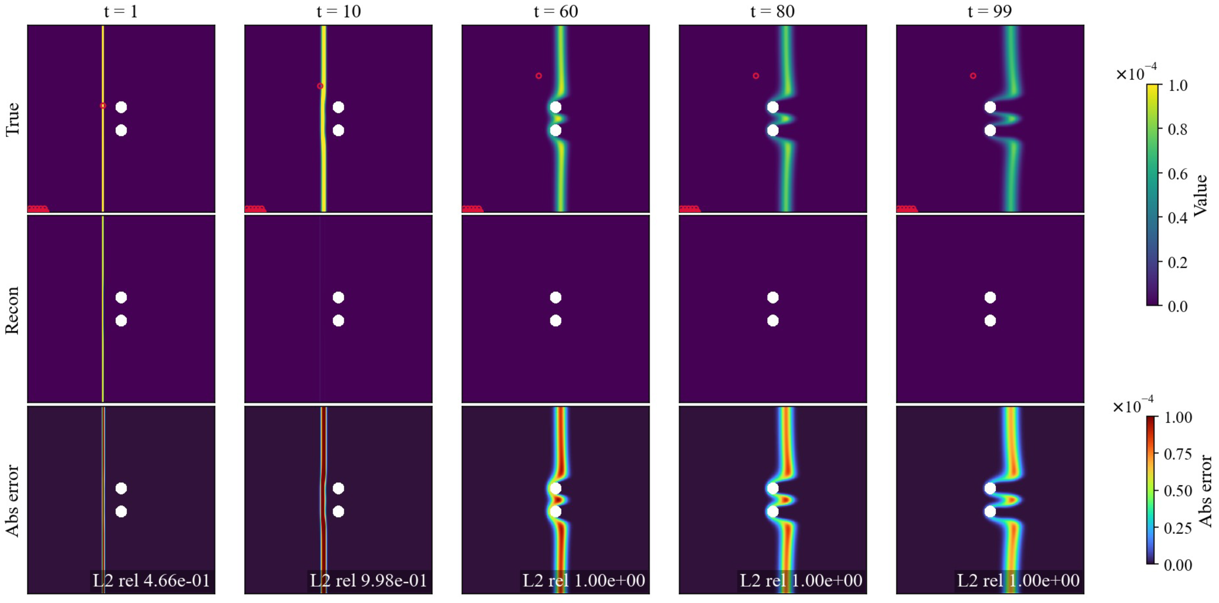
Given that the side-by-side cylinder setup has the highest spatial resolution and the longest sequence of time steps, we summarize the performance by the average runtime, as shown in Figure 17. All calculations were performed with an Apple M1 processor.
Figure 17 reports the average per-step runtime on a logarithmic scale for Local–QR under different mobility budgets J max and separation constraints d min , with Global–QR shown as a baseline. The main findings are as follows:
  • Overall trend with p. Across all panels, the Local–QR curves increase approximately monotonically with the number of sensors p; larger p yields longer per-step runtime. Moreover, the slope becomes markedly steeper as J max increases.
  • Dominant role of J max . For a fixed p, raising J max from 10 to 100 to 1000 produces order-of-magnitude growth in per-step runtime (an upward shift on the log scale), indicating that the candidate-neighborhood radius is the primary computational lever.
  • Minor impact of d min . Within each panel, the three Local–QR curves for d min { 0 , 10 , 100 } nearly coincide, suggesting that the minimum separation mainly affects placement diversity and numerical stability rather than runtime.
  • Comparison with Global–QR. The red baseline (Global–QR) is nearly flat across p and remains far below Local–QR, with the gap widening rapidly as J max grows: (i) J max = 10 : Local and Global are of the same order (tens of milliseconds), with Local slightly slower at larger p; (ii) J max = 100 : Local is roughly one order of magnitude slower; (iii) J max = 1000 : Local reaches the 10 3 ms range, substantially above Global.

3.5. Discussion

Since the phenomena observed in case 3 are nearly identical to cases 1 and 2, we focus the discussion on case 1, where the key performance trends can be clearly observed. As illustrated in Figure 5, Figure 6, Figure 7, Figure 8, Figure 9 and Figure 10, increasing the number of sensors and relaxing mobility constraints both enhance reconstruction accuracy, but excessive freedom in sensor movement ( J m a x = 50 ) can lead to unstable behavior and sensor clustering. The following analysis summarizes these dependencies in three aspects:
(1) The number of sensors p: As expected, increasing the number of sensors improves the accuracy of the reconstruction. With only one sensor, all methods fail after the first time step. p = 5 sensors allow for marginal improvement, but still result in rapid error growth. Ten and twenty sensors perform much better, especially when combined with small jumps. The number of sensors is determined by the number of POD modes r captured. A larger number of sensors allows for a more accurate representation of the dominant features of the system and leads to better reconstruction accuracy. This trend reflects the intrinsic rank limitation of the POD subspace: when p < r , the reduced measurement matrix C k U k becomes underdetermined and ill-conditioned, leading to the amplification of numerical errors during reconstruction.
(2) Jump constraint J m a x : The local QR strategy tends to select the locations with the highest modal energy greedily when there is no separation distance. J m a x results in sensor clustering, repeatedly choosing points in sharp modal regions such as local or domain boundary points. When J m a x is too large, the sensor movement becomes unstable and lacks temporal coherence, causing sensors to repeatedly track transient high-energy zones rather than maintaining spatial coverage. This behavior increases the condition number of C k U k , reducing numerical stability and leading to large fluctuations in reconstruction accuracy.
(3) Separation d m i n : When the separation constraint is relaxed ( d m i n = 0 ), sensors can cluster in high-information regions, improving performance. Larger separation values force the sensors to spread out, which can be detrimental when fewer sensors are available. A moderate separation constraint, however, helps maintain spatial diversity and reduces redundancy between neighboring sensors. This trade-off between coverage and redundancy explains why the optimal configuration occurs at small but nonzero d m i n , consistent with the balance between mobility cost and information gain in mobile sensor networks.
From a practical perspective, the proposed adaptive sensing framework can be implemented using autonomous or semi-autonomous mobile platforms, such as unmanned surface vehicles, aerial drones, or drifting buoys equipped with compact pollutant or particulate sensors. These systems can update their positions based on the proposed mobility-constrained QR strategy while maintaining communication through low-power wireless networks. The algorithm’s reliance on local movement and spatial separation constraints is consistent with realistic hardware limitations on battery life and motion range, making the approach feasible for large-scale environmental monitoring deployments.

4. Conclusions and Remarks

In this study, we proposed an adaptive sensor placement framework to reconstruct dynamic environmental pollution fields by combining proper orthogonal decomposition incrementally with QR-based selection limited by mobility. Unlike traditional global QR methods, our approach accounts for practical deployment constraints such as the number of sensors p, the minimum separation distance d min , and the maximum jump distance J max .
The proposed method demonstrates superior adaptability and robustness in three representative cases, particularly in scenarios with limited sensor resources or highly localized field variations. In particular, our experiments reveal that, under certain conditions, the local QR method with smaller d min can match the reconstruction accuracy of the global QR method, highlighting the advantage of localized optimization in time-varying systems. This study is well-suited for large-scale or limited monitoring tasks, such as urban air quality monitoring or the study of pollutant diffusion. Furthermore, our work contributes findings on how adaptive sensing strategies can balance physical constraints with numerical reconstruction performance. Through experimental analysis, we examined the influence of three key parameters and found that changes in condition number are the underlying reason for the observed differences in reconstruction performance.
This study developed an adaptive sensor placement framework that incrementally combines Proper Orthogonal Decomposition with a mobility-constrained QR-based selection strategy for reconstructing dynamic environmental fields. The framework is designed to bridge the gap between theoretical model reduction and the practical realities of environmental monitoring, where sensor mobility, communication, and energy limitations play a critical role. More broadly, this work contributes to the emerging intersection of environmental modeling, data-driven reduced-order modeling, and intelligent sensing. The proposed approach offers a new perspective for designing efficient observation systems capable of maintaining accuracy under physical constraints. In the future, extending this framework to nonlinear or multi-scale systems and coupling it with reinforcement learning–based decision policies could enable fully autonomous sensor networks for real-time environment monitoring.

Author Contributions

Conceptualization, A.L.; Methodology, D.X.; Software, A.L.; Formal analysis, D.C.; Resources, W.C.; Writing—review & editing, Q.L. All authors have read and agreed to the published version of the manuscript.

Funding

This research was supported by the Scientific Research Funding Project of Westlake University (Grant No. WU2024A001), generously donated by Li Duozhu, President of Dingheng Shipping Technology Co., Ltd. The authors gratefully acknowledge this support.

Data Availability Statement

The data and code used in this study are available from the authors upon reasonable request.

Conflicts of Interest

The authors declare no conflicts of interest.

References

  1. Mitchell, L.J.; Williamson, B.J.; Masden, E.A. Methods for highlighting ecological monitoring needs in data-sparse regions: A case study of impact assessment for multi-component infrastructure installations. Environ. Impact Assess. Rev. 2024, 105, 107433. [Google Scholar] [CrossRef]
  2. Masden, E.A.; McCluskie, A.; Owen, E.; Langston, R.H. Renewable energy developments in an uncertain world: The case of offshore wind and birds in the UK. Mar. Policy 2015, 51, 169–172. [Google Scholar] [CrossRef]
  3. Wayman, C.; Niemann, H. The fate of plastic in the ocean environment–a minireview. Environ. Sci. Process. Impacts 2021, 23, 198–212. [Google Scholar] [CrossRef]
  4. Brönmark, C.; Hansson, L.A. Environmental issues in lakes and ponds: Current state and perspectives. Environ. Conserv. 2002, 29, 290–307. [Google Scholar] [CrossRef]
  5. Tran-Nguyen, Q.A.; Le, T.M.; Nguyen, H.N.Y.; Nguyen, Q.T.; Trinh-Dang, M. Microplastics in the surface water of urban lakes in central Vietnam: Pollution level, characteristics, and ecological risk assessment. Case Stud. Chem. Environ. Eng. 2024, 9, 100622. [Google Scholar] [CrossRef]
  6. Yin, J.; He, B.; Fan, C.; Chen, R.; Zhang, H.; Zhang, Y. Drought-related wildfire accounts for one-third of the forest wildfires in subtropical China. Agric. For. Meteorol. 2024, 346, 109893. [Google Scholar] [CrossRef]
  7. Farid, A.; Alam, M.K.; Goli, V.S.N.S.; Akin, I.D.; Akinleye, T.; Chen, X.; Cheng, Q.; Cleall, P.; Cuomo, S.; Foresta, V.; et al. A Review of the Occurrence and Causes for Wildfires and Their Impacts on the Geoenvironment. Fire 2024, 7, 295. [Google Scholar] [CrossRef]
  8. Juwaied, A.; Jackowska-Strumillo, L. DL-HEED: A Deep Learning Approach to Energy-Efficient Clustering in Heterogeneous Wireless Sensor Networks. Appl. Sci. 2025, 15, 8996. [Google Scholar] [CrossRef]
  9. Stolkin, R.; Vickers, L.; Nickerson, J.V. Using environmental models to optimize sensor placement. IEEE Sens. J. 2007, 7, 319–320. [Google Scholar] [CrossRef]
  10. Bartolini, N.; Calamoneri, T.; Ciavarella, S.; Porta, T.L.; Silvestri, S. Autonomous mobile sensor placement in complex environments. ACM Trans. Auton. Adapt. Syst. (TAAS) 2017, 12, 1–28. [Google Scholar] [CrossRef]
  11. Sun, C.; Yu, Y.; Li, V.O.; Lam, J.C. Multi-type sensor placements in Gaussian spatial fields for environmental monitoring. Sensors 2019, 19, 189. [Google Scholar] [CrossRef]
  12. Nguyen, T.T.; Thanh, H.D.; Le, V.T. Optimization for the sensor placement problem in 3D environments. In Proceedings of the 2015 IEEE 12th International Conference on Networking, Sensing and Control, Taipei, Taiwan, 9–11 April 2015; IEEE: Piscataway, NJ, USA, 2015; pp. 327–333. [Google Scholar]
  13. Manohar, K.; Brunton, B.W.; Kutz, J.N.; Brunton, S.L. Data-driven sparse sensor placement for reconstruction: Demonstrating the benefits of exploiting known patterns. IEEE Control Syst. Mag. 2018, 38, 63–86. [Google Scholar]
  14. Williams, Z.; Soto Calvo, M.; Lee, H.S.; Aljber, M.; Jeong, J.S. A Low-Cost Autonomous Multi-Functional Buoy for Ocean Currents and Seawater Parameter Monitoring, and Particle Tracking. J. Mar. Sci. Eng. 2025, 13, 1629. [Google Scholar] [CrossRef]
  15. Riser, S.C.; Freeland, H.J.; Roemmich, D.; Wijffels, S.; Troisi, A.; Belbéoch, M.; Gilbert, D.; Xu, J.; Pouliquen, S.; Thresher, A.; et al. Fifteen years of ocean observations with the global Argo array. Nat. Clim. Chang. 2016, 6, 145–153. [Google Scholar] [CrossRef]
  16. Karnik, N.; Abdo, M.G.; Estrada-Perez, C.E.; Yoo, J.S.; Cogliati, J.J.; Skifton, R.S.; Calderoni, P.; Brunton, S.L.; Manohar, K. Constrained optimization of sensor placement for nuclear digital twins. IEEE Sens. J. 2024, 24, 15501–15516. [Google Scholar] [CrossRef]
  17. Yang, L.; Pang, Y.; He, X.; Wang, Y.; Kan, Z.; Song, X. An active learning-driven optimal sensor placement method considering sensor position distribution toward structural health monitoring. Struct. Multidiscip. Optim. 2024, 67, 1–23. [Google Scholar] [CrossRef]
  18. Hassani, S.; Dackermann, U. A systematic review of optimization algorithms for structural health monitoring and optimal sensor placement. Sensors 2023, 23, 3293. [Google Scholar] [CrossRef] [PubMed]
  19. Manohar, K.; Kutz, J.N.; Brunton, S.L. Optimal sensor and actuator selection using balanced model reduction. IEEE Trans. Autom. Control 2021, 67, 2108–2115. [Google Scholar] [CrossRef]
  20. Clark, E.; Askham, T.; Brunton, S.L.; Kutz, J.N. Greedy sensor placement with cost constraints. IEEE Sensors J. 2018, 19, 2642–2656. [Google Scholar] [CrossRef]
  21. Zhang, Q.; Wu, H.; Mei, X.; Han, D.; Marino, M.D.; Li, K.C.; Guo, S. A sparse sensor placement strategy based on information entropy and data reconstruction for ocean monitoring. IEEE Internet Things J. 2023, 10, 19681–19694. [Google Scholar] [CrossRef]
  22. Marcato, A.; Guiltinan, E.; Viswanathan, H.; O’Malley, D.; Lubbers, N.; Santos, J.E. Journey over destination: Dynamic sensor placement enhances generalization. Mach. Learn. Sci. Technol. 2024, 5, 025070. [Google Scholar] [CrossRef]
  23. Gao, H.; Hu, G.; Zhang, D.; Jiang, W.; Tse, K.; Noack, B.R. SiGAN: A 3D sensor importance deep generative model for urban wind flow field monitoring. Build. Environ. 2024, 262, 111787. [Google Scholar] [CrossRef]
  24. Andersson, T.R.; Bruinsma, W.P.; Markou, S.; Requeima, J.; Coca-Castro, A.; Vaughan, A.; Ellis, A.L.; Lazzara, M.A.; Jones, D.; Hosking, S.; et al. Environmental sensor placement with convolutional Gaussian neural processes. Environ. Data Sci. 2023, 2, e32. [Google Scholar] [CrossRef]
  25. Gao, H.; Liu, J.; Lin, P.; Hu, G.; Patruno, L.; Xiao, Y.; Tse, K.; Kwok, K. An optimal sensor placement scheme for wind flow and pressure field monitoring. Build. Environ. 2023, 244, 110803. [Google Scholar] [CrossRef]
  26. Wang, J.; Shen, T.; Zhao, D.; Zhang, F. MrDMD-Based Sensor Placement in Distributed Flow Estimation for the Design of the Artificial Lateral Line of an Underwater Robot. In Proceedings of the 2023 62nd IEEE Conference on Decision and Control (CDC), Singapore, 13–15 December 2023; IEEE: Piscataway, NJ, USA, 2023; pp. 4759–4765. [Google Scholar]
  27. Fareed, H.; Singler, J.R.; Zhang, Y.; Shen, J. Incremental proper orthogonal decomposition for PDE simulation data. Comput. Math. Appl. 2018, 75, 1942–1960. [Google Scholar] [CrossRef]
  28. Fischer, H.; Roth, J.; Wick, T.; Chamoin, L.; Fau, A. MORe DWR: Space-time goal-oriented error control for incremental POD-based ROM for time-averaged goal functionals. J. Comput. Phys. 2024, 504, 112863. [Google Scholar] [CrossRef]
  29. Feng, L.H.; Wang, J.J.; Pan, C. Proper orthogonal decomposition analysis of vortex dynamics of a circular cylinder under synthetic jet control. Phys. Fluids 2011, 23, 014106. [Google Scholar] [CrossRef]
  30. Ren, J.; Mao, X. Uncertainty transmission of fluid data upon proper orthogonal decompositions. Phys. Fluids 2023, 35, 071702. [Google Scholar] [CrossRef]
  31. Berkooz, G.; Holmes, P.; Lumley, J.L. The proper orthogonal decomposition in the analysis of turbulent flows. Annu. Rev. Fluid Mech. 1993, 25, 539–575. [Google Scholar] [CrossRef]
  32. Kim, Y.H. Greedy sensor selection based on QR factorization. EURASIP J. Adv. Signal Process. 2021, 2021, 1–13. [Google Scholar] [CrossRef]
  33. He, Q.; Tartakovsky, A.M. Physics-informed neural network method for forward and backward advection-dispersion equations. Water Resour. Res. 2021, 57, e2020WR029479. [Google Scholar] [CrossRef]
  34. Wang, C.; Wu, H.; Wang, N.; Ye, Z. A Novel Ship Fuel Sulfur Content Estimation Method Using Improved Gaussian Plume Model and Genetic Algorithms. J. Mar. Sci. Eng. 2025, 13, 690. [Google Scholar] [CrossRef]
  35. Meng, J.; Li, C.; Martin, R.V.; van Donkelaar, A.; Hystad, P.; Brauer, M. Estimated long-term (1981–2016) concentrations of ambient fine particulate matter across North America from chemical transport modeling, satellite remote sensing, and ground-based measurements. Environ. Sci. Technol. 2019, 53, 5071–5079. [Google Scholar] [CrossRef] [PubMed]
  36. Weymouth, G.D.; Font, B. WaterLily. jl: A differentiable and backend-agnostic Julia solver for incompressible viscous flow around dynamic bodies. Comput. Phys. Commun. 2025, 315, 109748. [Google Scholar] [CrossRef]
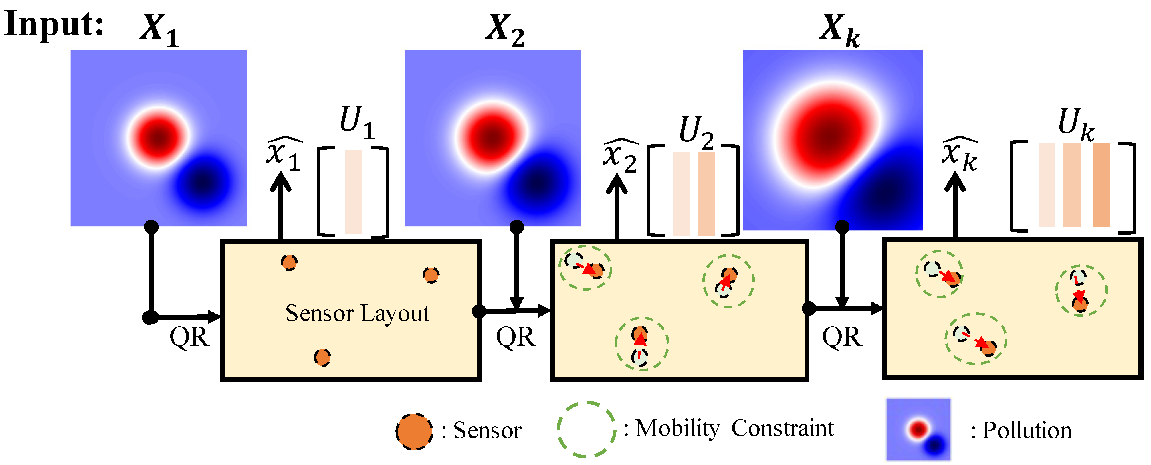
Figure 1. The framework of online sparse sensors selection with local mobility constraint.
Jmse 13 01995 g001
Figure 2. (A) The value of the first step of the pollution field (t = 1 s). (B) Index of sensors in the layout, corresponding to 101 × 101 grids.
Jmse 13 01995 g002
Figure 3. Left: The PM2.5 distribution in the American inland 2016/01. Right: Corresponding sensor grids. The 3328 sensors were sorted first by increasing latitude, and, for sensors at the same latitude, by increasing longitude. Panels (A,B) use the same x- and y-axis ranges.
Jmse 13 01995 g003
Figure 4. Flow past side-by-side cylinders.(A.1A.3) Evolution of the scalar field at different dimensionless times. (B) Distribution of sensor IDs, with blank regions inside the cylinders. (C.1C.3) Corresponding vorticity fields. (D) Time history of the integrated scalar mass, showing its conservation over simulation steps. Panels (A.1A.3C.1C.3) use a 512 × 512 grid.
Jmse 13 01995 g004
Figure 5. Comparison between local and global QR methods under different settings of p, J max , and d m i n in the plume case. Panels (B.1C.3) share the same y-axis scale as panel (A.1A.3).
Jmse 13 01995 g005
Figure 6. The performance of the global QR under the setting of p = 10 in the plume case. All panels are used the same as the Figure 2.
Jmse 13 01995 g006
Figure 7. The global QR sensor positions under the setting of p = 10 in the plume case.
Jmse 13 01995 g007
Figure 8. The optimal sensor positions under the setting of J m a x = 50 , with p = 10 and d m i n = 1 .
Jmse 13 01995 g008
Figure 9. The performance under the setting of J m a x = 50 , with p = 10 and d m i n = 0 .
Jmse 13 01995 g009
Figure 10. The optimal sensor positions under the setting of J m a x = 50 , with p = 10 and d m i n = 0 .
Jmse 13 01995 g010
Figure 11. The performance of different sensor numbers and max jump grids in local QR in the PM2.5 case. Panels (A.1D.3) show performance with 1, 5, 10, and 20 sensors, respectively.
Jmse 13 01995 g011
Figure 12. The results of incremental global QR within 20 sensors.
Jmse 13 01995 g012
Figure 13. The results of incremental local QR within 20 sensors in 500 km jump constraints and a separation distance of 100 km.
Jmse 13 01995 g013
Figure 14. Performance of the Local QR method in case 3: p = 1 , p = 10 , and p = 50 , shown in (A)–(C), respectively. Subplots (A,B) share the same colorbar. Each subplot title reports the reconstruction error obtained using the corresponding global method.
Jmse 13 01995 g014
Figure 15. The performance under the setting of the global QR within p = 50 . The circles indicate the positions of the sensors.
Jmse 13 01995 g015
Figure 16. The performance under the setting of J m a x = 10 , with p = 50 and d m i n = 10 . The circles indicate the positions of the sensors.
Jmse 13 01995 g016
Figure 17. Average computation time for the side-by-side cylinders case under different mobility and separation settings.
Jmse 13 01995 g017
Table 1. Condition number of [ C k U k ] at each time step and sensor mobility metrics under the setting p = 10 .
MetricGlobal QR J max = 50 , d min = 0 J max = 50 , d min = 1
Condition Number at Time Step t k
t 0 1.001.001.00
t 1 2.99 1.53 × 10 11 4.24
t 2 3.90 6.93 × 10 21 5.52
t 3 4.416.13
t 4 4.374.10
t 5 4.29 1.35 × 10 82 5.89
Sensor Movement Metrics (Grid Units)
L ¯ 14.9621.0120.39
L max 84.7435.3641.48
Table 2. Condition numbers of [ C k U k ] at each step in case 2 within the setting of J m a x = 500 and p = 20 .
MetricGlobal QR d min = 100 d min = 10 d min = 0
Condition Number at Time Step t k
01.001.001.001.00
11.731.581.692.78
22.451.401.6630.6
32.901.701.626.94 × 1016
44.982.182.193.61 × 1016
55.402.592.569.93 × 1032
610.13.763.963.29 × 1033
712.23.814.57
811.34.324.79
911.44.884.54
1011.68.897.97
11987698879
Sensor Movement Metrics (km)
L ¯ 395.4216.6211.6102.8
L m a x 3313.5498.7493.0487.5
Table 3. Sensor mobility metrics under the setting p = 50 in case 3.
MetricGlobal QR J max = 100 , d min = 10 J max = 1000 , d min = 10
Sensor Movement Metrics (Grid Units)
L ¯ 47.028.1462.26
L max 554.15100553
Disclaimer/Publisher’s Note: The statements, opinions and data contained in all publications are solely those of the individual author(s) and contributor(s) and not of MDPI and/or the editor(s). MDPI and/or the editor(s) disclaim responsibility for any injury to people or property resulting from any ideas, methods, instructions or products referred to in the content.