Abstract
The introduction of Maritime Autonomous Surface Ships (MASS) and the accelerating digitalization of ports require precise and dynamic analysis of traffic conditions. However, conventional marine traffic analyses have been limited to low-resolution grids and static density visualizations without fully integrating vessel direction and speed. To address this limitation, this study proposes a traffic flow visualization model that incorporates dynamic maritime traffic structure. The model integrates density, dominant direction, and average speed into a single symbol, thereby complementing the limitations of static analyses. In addition, high-resolution grids of approximately 90 m were applied to enable detailed analysis. AIS data collected between 2022–2023 from the coastal waters of Mokpo, South Korea, were preprocessed, aggregated into grid cells, and analyzed to estimate representative directions (at 10° intervals) as well as average speeds. These results were visualized through color, thickness, length, and direction of arrows. The analysis showed high-density, low-speed traffic patterns and starboard-passage behavior in port approaches and narrow channels, while irregular directions with low density were observed in non-standard routes. The proposed model provides a visual representation of dynamic traffic structures that cannot be revealed by density maps alone, thus offering practical applicability for MASS route planning, VTS operation support, and risk assessment.
1. Introduction
With the continuous growth of global maritime trade, the enlargement of vessels, the increasing complexity of shipping logistics, and the digitalization of port facilities, the marine traffic environment has been evolving toward greater complexity and precision [1]. In particular, vessel traffic tends to be concentrated in port approaches, coastal waters, and narrow channels, where existing traffic management systems face limitations in capturing traffic flow patterns and providing detailed responses [2]. These circumstances emphasize the need for fundamental technologies that can structure and quantitatively analyze marine traffic data.
Recently, the development and introduction of Maritime Autonomous Surface Ships (MASS) have further increased the demand for a more refined traffic analysis [3]. MASS requires structured quantitative information on surrounding traffic conditions to support autonomous navigational decisions, which highlights the importance of high-resolution traffic analysis systems [4]. At the same time, port operations are rapidly shifting toward digitalization and automation, creating strong demand for structured information systems that can support the establishment of smart ports [1,5]. With the spread of concepts such as digital twins, e-Navigation, and maritime big data platforms, marine traffic analysis must move beyond simple statistical density evaluations and toward integrated analytical frameworks that incorporate directionality and predictive capability.
These technological and environmental changes stress the need to develop new information models to overcome the limitations of conventional approaches and respond to diverse operational and regulatory-related requirements. Marine traffic analysis has traditionally been applied to density evaluation, route extraction, predictive modeling, and risk assessment [6]. In particular, Vessel Traffic Services (VTS) and port authorities utilize Automatic Identification System (AIS) data to quantitatively monitor traffic flows and detect anomalies, which ultimately leads to accident prevention and efficient port management [7]. However, conventional analyses have primarily focused on static density measures and have not sufficiently incorporated dynamic factors such as vessel direction and speed.
Most grid-based traffic models employ low-resolution grids of more than 1 km, which restricts their effectiveness in complex areas such as harbors and narrow channels, where fine-scale analysis is required [8,9,10]. Furthermore, flow maps that simultaneously integrate passage routes, directionality, and speed characteristics are rarely implemented. These limitations highlight the need for improved traffic models.
Previous studies based on AIS data have advanced marine traffic analysis in areas such as density evaluation, route extraction, traffic flow visualization, predictive modeling, and risk assessment [6,11]. While these studies have laid the foundation and expanded the scope of applications, they also share common limitations, including the reliance on low-resolution grids, a focus on static analysis, and visualization methods primarily on color-coded heatmaps. These issues are examined in more detail in the following literature review.
Research that aggregates AIS data into grid cells to visualize static traffic density has been actively conducted since the early stages of marine traffic studies. Kim et al. [8] calculated traffic density by incorporating length overall (LOA), speed over ground (SOG), and passage counts, demonstrating the potential of quantitative analysis using high-resolution grids. Y.-J. Kim et al. [12] calculated vessel occupancy time from AIS data and visualized major routes by applying logarithmic transformation and color-stretching techniques. Similarly, Lee et al. [13] presented a grid-based visualization model with 30 m resolution that integrated density, direction, and flow elements, but their study did not include the analysis or visualization of speed. Nevertheless, most of these studies focused on static heatmap-based visualization, with limited attempts to depict traffic flow by integrating direction and speed.
Several studies have also been conducted to extract or cluster major routes using AIS trajectory data. Son et al. [14] applied a particle swarm optimization (PSO) algorithm to derive representative route structures. Huang et al. [15] proposed an automatic method for extracting routes through multidimensional clustering based on DBSCAN. A study using Soft-DTW clustering has also modeled the central lines of major routes in port approach waters [16]. While these approaches are effective for clustering and identifying route patterns, they differ in nature from grid-based flow analysis or direction- and speed-based visualization, thus remaining limited in directly representing traffic flow structures.
Attempts have also been made to quantitatively evaluate marine traffic flow conditions. W.-J. Son & Cho [10] estimated the optimal navigation channel width around offshore wind farms based on traffic density and collision probability. Luong et al. [17] developed maritime risk maps by introducing the Marine Traffic Hazard Index to quantify risk. Sui et al. [18] applied network analysis based on the Visibility Graph method to define multiple traffic states and proposed a statistical evaluation framework. However, these studies mainly focused on static density indicators or risk classification and did not provide integrated flow analysis that incorporates time, speed, and directional information.
More recently, deep learning methods have been employed to predict AIS-based marine traffic flows. X. Wang & Xiao [19] improved trajectory prediction accuracy using a CNN-LSTM-SE architecture. Wang et al. [20] compared and analyzed various deep learning models to propose an optimized model for marine traffic flow prediction. Further contributions include the use of deep learning models to enhance vessel trajectory prediction with AIS data and the application of clustering combined with deep recurrent neural networks for anomalous behavior detection [21,22]. These studies focused on improving routes prediction performance but were not directly related to spatial grid-based visualization or explicit representation of flow direction.
Taken together, previous studies confirm that various AIS-based maritime traffic analyses have been conducted, yet several limitations are still evident. Firstly, many studies employed low-resolution grids of 500 m–1 km, which restricts fine-scale analysis in complex local waters such as narrow channels and port approaches. At such resolutions, it is difficult to support detailed decision-making for autonomous ships, including route planning or collision avoidance. Secondly, most of the previous research were limited to static density analysis without reflecting dynamic characteristics such as vessel direction and speed. This constrains the ability to explain structural traffic flow features or assess hazardous situations in detail. Thirdly, visualization methods have largely relied on color-based heatmaps, which make it difficult to represent density, direction, and speed in an integrated manner.
To overcome these limitations, this study develops a marine traffic flow visualization model with the following distinctive features. First, the model introduces a traffic flow visualization model that extends beyond density-centered approaches, enabling simultaneous expression of vessel direction and speed at the grid level. Second, the model adopts an arrow-based visualization scheme in which arrow thickness represents density, length indicates speed, and angle shows dominant direction. Third, a high-resolution 90 m grid is applied, allowing much more effective analysis of complex waters such as narrow channels and port approaches. These characteristics provide a useful foundation for satisfying operational needs such as route planning, collision avoidance, and VTS support in the context of MASS. To sum up, unlike conventional density-based approaches that only count the number of vessels within a region, the proposed model simultaneously integrates traffic density, average speed, and dominant direction into a unified arrow symbol. By applying this integrated flow representation on a high-resolution 90 m grid, the model addresses the limitations of traditional methods and provides more comprehensive insights into dynamic traffic structures.
This study applies the proposed model to real AIS data to derive results comparable with conventional analyses and to verify its applicability. The analysis evaluates whether the model accurately reflects complex traffic structures and reveals dynamic characteristics that were difficult to identify using existing approaches. The proposed model also demonstrates potential applications in MASS navigation support, port management, and risk assessment, providing both academic and practical significance.
The remainder of this paper is structured as follows. Section 2 describes the design concept of the proposed marine traffic flow visualization model and data processing procedures. Section 3 presents visualization and analysis results obtained by applying the model to real-world AIS data. Section 4 summarizes the main findings, discusses limitations, and suggests directions for future research.
2. Marine Traffic Flow Visualization Model Development
This section describes the data and analytical procedures used to construct the proposed marine traffic flow visualization model. First, the study area and characteristics of the AIS dataset are introduced, followed by preprocessing steps undertaken to ensure data reliability. The method for defining and calculating grid-based traffic density is then explained, along with the procedure for deriving the traffic flow diagram. Finally, the visualization approaches for both density and flow are described. Through these steps, AIS data are structured to enable simultaneous quantitative and visual analysis of traffic conditions in the study area.
2.1. AIS Data
This study is based on the analysis of AIS data. AIS is equipment that automatically transmits a vessel’s positional and navigational information, which can be received by nearby ships and coastal authorities, serving as an essential system for maritime safety and efficient traffic management. According to Regulation 19 of Chapter V of the International Convention for the Safety of Life at Sea (SOLAS), AIS is mandatory for international voyages of vessels of 300 gross tonnage or more, non-international voyages of vessels of 500 gross tonnage or more, and all passenger ships regardless of size. AIS messages include basic identification information (MMSI, IMO number, call sign, vessel name, vessel type) as well as navigational attributes such as latitude and longitude, Coordinated Universal Time (UTC) timestamp, Speed Over Ground (SOG), Course Over Ground (COG), heading, navigation status, draft, destination, and Estimated Time of Arrival (ETA). With these multidimensional attributes, AIS data can be used not only to capture large-scale maritime traffic distribution, but also to analyze detailed navigational behavior of individual vessels.
For this study, AIS data collected from the coastal waters near Mokpo between 1 January 2022 and 31 December 2023—two years in total—were utilized. While the data points were recorded at the second level, irregular transmission intervals and outliers required preprocessing before analysis. All vessels passing through the study area were included regardless of ship type, but vessels with speeds under 2 knots were excluded, as they are unlikely to be underway. This is due to the possibility that some ships may not change their AIS navigation status to “at anchor” or input any other incorrect information.
The study area covers approximately 50 km of coastal waters near Mokpo in Jeollanam-do, a critical node of West Sea coastal routes and a region with converging island routes. This area represents a highly complex traffic environment, with port-entry vessels, coastal ferries, and fishing vessels all operating simultaneously [23]. In particular, port approaches to the North Port, New Mokpo Port, as well as adjacent narrow channels, experience high levels of traffic density and frequent interference between vessel routes. Such conditions provide an appropriate setting for applying and validating the proposed traffic model. Figure 1 shows the target area near Mokpo.
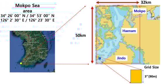
Figure 1.
Target area.
For spatial analysis, the study area was divided into grid cells of approximately 90 m × 90 m. Figure 2 presents an example in which the Mokpo region, one of the high-density traffic areas within the target area, was divided using this grid size. This illustration presents the level of resolution used for the grid. This grid size was deliberately chosen because it roughly corresponds to the length of medium-sized vessels, ensuring that the traffic information produced by the model is directly meaningful for route planning and navigational decision-making. Here, the term “resolution” refers not to the technical capacity of AIS equipment itself, but to the spatial resolution determined by the applied grid size in traffic modeling. The chosen resolution balances the positional accuracy of AIS data (approximately 10 m) while providing sufficient detail to represent the complexity of harbor waters. Compared with previous studies that typically employed grid sizes of 500 m to 1 km, the grid framework in this study offers greater applicability for fine-scale analysis in local areas such as narrow channels and port approaches.
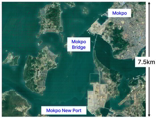
Figure 2.
Grid division without data input.
Within each grid cell, vessel passage counts, average speed, and dominant direction were aggregated to enable simultaneous analysis of traffic density and flow. Grid indexing (,) was defined based on the upper-left coordinate of the study area, as shown in Equation (1).
where i and j denote the grid indices along the latitude and longitude directions, respectively; top_left_lat and top_left_lon represent the latitude and longitude of the upper-left corner of the study area; and grid_interval indicates the grid resolution (90 m in this study).
The vast AIS dataset was structured through this grid division, providing a foundation for a quantitative analysis of traffic density and flow in both temporal and spatial units.
2.2. Data Preprocessing
The raw AIS dataset required multiple preprocessing steps to ensure reliability and analytical consistency. First, critical attributes such as timestamp, MMSI, longitude, latitude, and vessel speed were extracted from the original AIS messages. Based on their temporal properties, the extracted records were divided into daily sets covering all vessels within the study area. These data were then reorganized by vessel MMSI, where each vessel’s dataset was chronologically sorted to construct continuous trajectory records.
To enhance data accuracy, abnormal or inconsistent points were identified and removed. Data points located on land were discarded using a land–sea mask, while discontinuities in vessel movements were detected by examining spatial and temporal intervals between consecutive points. For example, if the distance between two successive AIS messages exceeded one nautical mile, the trajectory segment was regarded as discontinuous and got excluded from continuous analysis. Following this process, vessel trajectories were segmented at abnormal points and reconstructed to ensure logical continuity. Each reconstructed segment was labeled and stored in a structured format for subsequent analysis.
Additional preprocessing procedures were applied to refine the dataset further. Missing or erroneous values were removed, and coordinate data were projected onto a uniform spatial reference system to enable consistent grid indexing. Temporal aggregation was performed through hourly and daily binning, which aligned the dataset with the spatiotemporal resolution required for grid-based analysis. Finally, incoming data was filtered by vessel type or size where necessary in order to facilitate targeted analysis of specific ship groups. Figure 3 summarizes the overall workflow of these preprocessing steps.
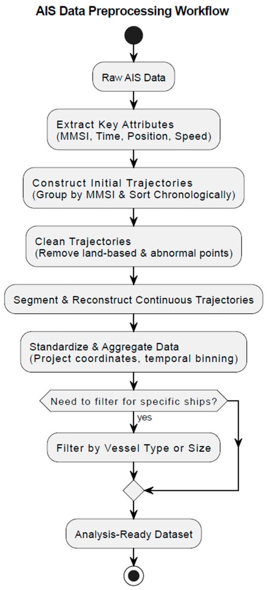
Figure 3.
AIS data preprocessing work flow chart.
2.3. Traffic Density
This section describes the traffic density component of the proposed traffic model and explains how it is represented through color-based visualization. Traffic density was calculated by quantitatively aggregating the number of vessel passages through each grid cell within a given time unit. This approach allows the spatial distribution of vessel activity to be visualized across the study area, which is useful for identifying congested routes or potential traffic hotspots. The density value for each grid cell is defined as shown in Equation (2).
Here, represents the number of vessel passages aggregated within grid cell (i, j) for a specified time interval. This value includes repeated passages of the same vessel and can be aggregated on a daily, monthly, or yearly basis depending on the purpose of the analysis.
In conventional traffic engineering, the flow–density (F–D) diagram is commonly used to describe the relationship between traffic flow—the number of vehicles passing a certain road segment per unit time—and density, which represents the number of vehicles occupying the road segment at a given moment [24,25]. This relationship is fundamental for identifying traffic states and determining the critical capacity of a roadway.
In maritime environments, however, traffic density is analyzed not along a linear road segment but over an area grid, since vessel movement occurs in a two-dimensional space. Consistent with many previous studies, the marine traffic density adopted in this study represents the number of vessels passing through a specific grid cell within a defined time period, which inherently incorporates a temporal component [8,9,10]. Therefore, although the form of representation differs, the concept of marine traffic density in this study is analogous to that of traffic flow in land-based transportation engineering. In this research, the analysis was performed using two years of AIS data, providing an aggregated view of vessel movements that reflects long-term traffic characteristics.
For visualization, the values were classified and color-coded into 15 levels (Level 1–15). Low-density areas were represented by blue–green tones (Level 1–5), medium-density areas by yellow tones (Level 6–10), and high-density areas by red tones (Level 11–15). This design allows users to intuitively recognize areas with concentrated vessel activity. For instance, Level 1 indicates lowest-density cells with the fewest passages, while Level 15 represents cells with the highest traffic density within the study area.
Such classification not only differentiates density values by color but also enables users to perceive relative density levels in a stepwise manner. Figure 4 illustrates an example of traffic density visualization with this classification applied to the grid, while Table 1 provides the corresponding RGB color values for each level (Level 1–15). Through this scheme, users can easily identify the degree of traffic density in a given grid cell by its color.
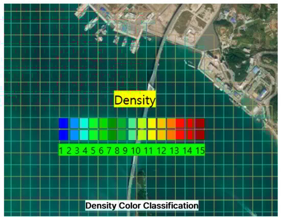
Figure 4.
Traffic density visualization method on grid.

Table 1.
Color classification scheme for traffic density visualization.
2.4. Traffic Flow
Following the previous section that described traffic density, this section explains the traffic flow diagram, which integrates traffic density into a unified representation. Traffic flow is defined as a visualization technique that simultaneously expresses vessel density, dominant movement direction, and average speed within a specific sea area. While density analysis only provides a static indicator of vessel distribution and concentration, the flow diagram incorporates directionality and speed, thereby capturing the dynamic characteristics of actual traffic. Thus, density indicates “the number of vessels passed through a given grid,” whereas the flow diagram shows “in which direction and at what speed they moved,” enabling a more intuitive and precise interpretation of marine traffic. Conceptually, the proposed traffic flow is defined as information that represents the overall stream of vessel movement by combining direction, speed, and density—similar to how fluid motion can be described by both its direction and intensity.
The traffic flow visualization model was designed to visualize three elements—direction, speed, and density—using a single arrow symbol. In each grid cell, vessel traffic characteristics are simultaneously represented by the thickness, length, and angle of an arrow, allowing users to intuitively grasp the traffic situation with a single symbol.
- (1)
- Traffic Direction
First, the traffic direction was determined by splitting the entire 360° grid into 36 sectors at 10° intervals, as shown in Equation (3).
where COG denotes the instantaneous course over ground of a vessel in degrees (0–360), and s is the index of the directional sector (0–35).
Each AIS sample was then classified into its corresponding sector, and the sector with the largest number of samples was defined as the dominant direction, as shown in Figure 5 and illustrated in Equation (4).
where is the dominant directional sector in grid cell (i, j), and represents the number of AIS samples in grid cell (i, j) that fall into sector s.
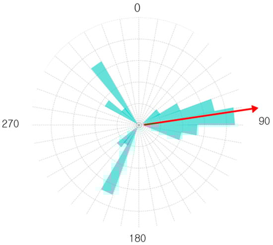
Figure 5.
Example of determining dominant traffic flow direction.
The use of a dominant direction approach offers the advantage of clearly identifying the prevailing traffic orientation within each grid cell; however, it also has limitations in areas where bidirectional or crossing traffic flows coexist. In such cases, no single direction emerges as dominant. While this reflects a methodological limitation, the resulting mixed patterns themselves can be considered an advantage, as they reveal the inherent complexity of local traffic conditions and provide meaningful insights for navigators. The potential for methodological improvements to address these limitations will be explored in future research.
- (2)
- Traffic Speed
Second, the representative speed of traffic was calculated as the average speed of AIS samples within the dominant direction in each grid cell, as defined in Equation (5).
where SPD denotes the vessel’s instantaneous speed over ground (in knots);
is the number of AIS samples within the dominant sector in grid cell (i, j); and represents the average speed of vessels in grid cell (i, j) along the dominant sector .
To reflect navigational characteristics, the representative speeds were categorized into five intervals: 0 ≤ kts < 4, 4 ≤ kts < 8, 8 ≤ kts < 12, 12 ≤ kts < 16, 16 kts (Table 2). In the visualization stage, these intervals were mapped to the relative length of arrows, enabling intuitive distinction between low-speed and high-speed navigation zones. In this context, SPD categorization into five intervals was designed to capture practical navigation characteristics, where arrow length serves as a visual proxy for relative vessel speed in each cell.
Table 2.
Classification of traffic density and speed levels.
- (3)
- Traffic Density
Finally, traffic density was expressed by regrouping the values defined in Section 2.3 (Levels 1–15) into five broader categories: Levels 1–3, 4–6, 7–9, 10–12, and 13–15 (Table 2). In this model, density corresponds to the total AIS sample counts per grid cell, reflecting passage frequency. While 15 levels were originally used for detailed classification in the traffic density model, these were consolidated into five categories for readability.
The traffic flow diagram was visualized by combining the density heatmap with flow arrows derived from traffic direction and speed. The arrow angle corresponded to the central angle of the dominant direction sector. The arrow length was proportional to the representative average speed, while its thickness reflected the five density categories. In addition, a 15-level color classification was applied to the background density heatmap, allowing density and flow patterns to be interpreted together in an integrated manner (Figure 6, Figure 7 and Figure 8).
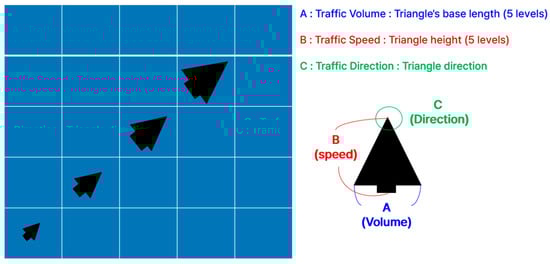
Figure 6.
Description of traffic flow elements.
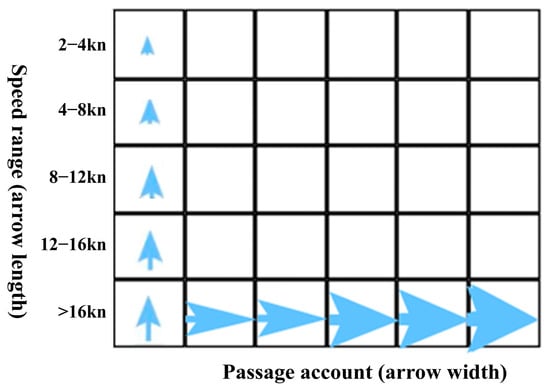
Figure 7.
Arrow-based visualization scheme of traffic flow.
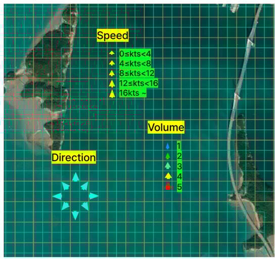
Figure 8.
Visualization of traffic flow symbols on grid.
2.5. Data Scaling Method
However, the actual distribution of AIS data tends to be excessively concentrated within certain ranges, particularly in low-speed intervals or grid cells with small passage counts. When equal-interval classification is applied in such cases, samples are heavily skewed toward the lower ranges, leading to visual distortion. For example, more than half of the total data may fall into the lowest category, while the upper categories remain underrepresented or diluted, as illustrated in Figure 9.
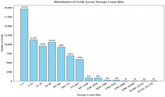
Figure 9.
Passage counts distribution using equal-interval bins.
To mitigate this issue, this study applied a log-binning approach. Log binning involves transforming the raw values onto a logarithmic scale and then dividing them into equal intervals, thereby defining class boundaries that distribute small and large values more evenly [26]. The classification procedure was defined according to Equations (6)–(8). By maintaining equal intervals on a logarithmic scale, this method effectively handles exponentially increasing data distributions.
where and denote the minimum and maximum traffic density values observed in the study area; and are their logarithmic values; is the number of bins used to divide the logarithmic scale; represents the i-th boundary value on the logarithmic scale; and is the i-th bin range mapped back to the original scale.
The log-binned intervals obtained through this procedure were subsequently used in the mapping stage, where visual attributes were assigned to each interval. Mapping is defined as the process of linking the intervals to arrow thickness, color levels, or legend values according to the visualization scheme described earlier. For example, when passage counts fall into a lower interval, relatively thinner arrows are assigned, whereas higher intervals are represented by thicker arrows, thereby visually highlighting differences in traffic volume. The same principle was applied to speed values, where higher average speeds in each interval were mapped with longer arrow lengths. In this process, the boundary values defined by log binning served to balance the data distribution, while the mapping stage translated these results into visual symbols that could be intuitively interpreted by users. Through this procedure, the proposed traffic flow diagram enables not only the representation of absolute values but also relative and comparative interpretation that reflects the characteristics of the underlying distribution.
2.6. Summary of the Proposed Traffic Model
The proposed traffic model integrates both density and flow into a unified representation. While conventional traffic density models have been limited to static visualization based on simple counts of vessel passages within grid cells, the present model incorporates vessel direction and speed to capture a more dynamic and integrated traffic structure. For this purpose, density values calculated for each grid cell are expressed through color intervals and arrow thickness, while flow elements are visualized by arrow direction and length, providing a combined representation within the same spatial framework. Unlike traditional single-indicator analyses, this structure enables simultaneous interpretation of both density distribution and dynamic flow characteristics.
In particular, the proposed model is applicable even in areas that require detailed interpretation, such as narrow channels and port approaches, through high-resolution spatial analysis at a 90 m grid scale. By applying a log-binning method, the model alleviates data skewness, ensuring a balanced representation of a wide range of passage counts and speed intervals. Compared with traditional density-focused approaches, this model enhances the quantitative and visual interpretability of traffic conditions.
Thus, the proposed traffic model extends beyond a simple density map to establish a new analytical framework with diverse applications, including congestion prediction, route design assessment, and MASS navigation decision support. The next section applies the model to actual AIS data to demonstrate the visualization results and verify the effectiveness and applicability of the proposed methodology.
3. Visualization Results
This section presents the visualization results of applying the proposed traffic model (density and flow) to AIS data in the study area. The results confirm how traffic density and flow structures appear at the grid level and allow comparative analysis of characteristics across different subregions. The visualizations first show the overall distribution across the entire study area, followed by detailed analyses of specific traffic-concentrated zones such as port approaches, narrow channels, and offshore connecting routes.
3.1. AIS Data Distribution in the Study Area
Based on the preprocessed AIS data, the baseline traffic distribution of the study area was first examined. Figure 10 overlays two years of AIS data collected in the Mokpo coastal region onto a map, showing that the processed position reports form linear patterns along actual shipping routes. As illustrated, traffic is concentrated around port approaches and narrow channels, particularly along the approach routes connecting North Port and New Mokpo Port, the narrow channel near Mokpo Bridge, and the offshore routes. In contrast, the outer coastal areas and island waters show sparse distribution, clearly differentiating between major and secondary routes. These results not only confirm that the study area is a traffic-intensive region where West Sea coastal and island routes intersect, but also validate that it provides suitable conditions for applying and verifying the proposed density and flow visualization model. Based on this data distribution, the next subsection presents density and flow results derived from the calculation procedures described earlier.
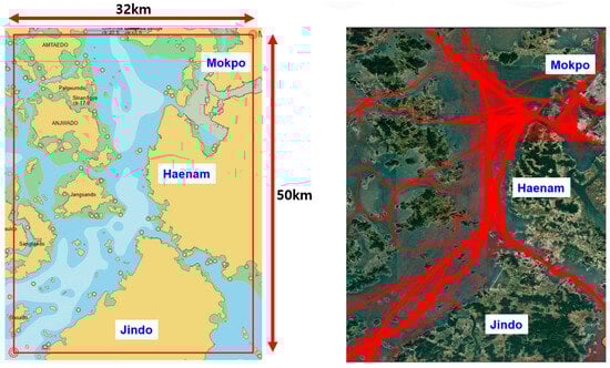
Figure 10.
Visualization of AIS data on target area.
3.2. Visualization Results of Traffic Density and Flow
This section presents the visualization results of traffic density and flow in the study area. First, the overall results for the entire region are shown, followed by detailed analyses of major traffic-concentrated zones. The study area exhibited clear spatial differences in traffic distribution. In some zones, vessel passages were highly concentrated, resulting in high density, while the density was relatively low in other zones. However, high density did not necessarily imply uniform characteristics, as speed and directional patterns varied even across different high-density zones. Such differences are difficult to identify from density maps alone but became more apparent when flow diagrams were presented in combination. Therefore, visualizations that integrate both density and flow serve as an important tool for interpreting marine traffic conditions in both quantitative and qualitative terms.
First, as shown in the traffic density and flow maps (Figure 11), the major inbound and outbound routes connecting Mokpo Port and New Mokpo Port, the narrow channel near Mokpo Bridge, and the entrance channel to Mokpo Port, all highlighted by the red box, appeared as high-density zones corresponding to the upper levels of the classification. This indicates that these areas serve as the core transit routes of the port, where a large number of vessels are concentrated. On the contrary, peripheral waters such as those around islands or along the outer offshore boundaries were widely distributed within the low-density range (Levels 1–5). These areas exhibited relatively low traffic volumes, suggesting that their overall influence on traffic is limited, which ultimately highlights distinct differences in utilization within the study area.
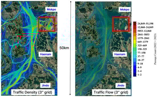
Figure 11.
Visualization of traffic density and traffic flow (whole target area).
The first enlarged area (Figure 12) covers approximately 7 km of the Mokpo waterway, including the main route connecting Mokpo Port and New Mokpo Port as well as the adjacent narrow channel. The results indicated high-density levels of 8 or above along the entire main route, while surrounding waters outside the main route also showed density levels above 5. In the flow diagram, many arrows appeared to be thick and short, reflecting areas with both high passage counts and low average speeds. This pattern can be interpreted as representing congestion and delays during port entry and departure. In addition, at junctions where routes diverged or merged, the arrows displayed dispersed orientations, broadly revealing the complexity of traffic congestion in these zones. The red box in the figure highlights the area with the most pronounced density, which is further enlarged and analyzed in greater detail in the following subsection.
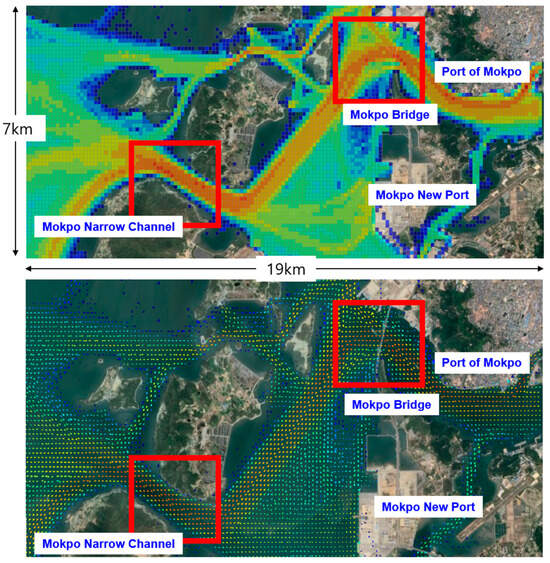
Figure 12.
Visualization of traffic density and traffic flow (close view, ~7 km: Mokpo approach area).
The second enlarged area covers approximately 2 km around Mokpo Bridge and the adjacent narrow channel near Mokpo Port. The density results indicated high levels across most parts of the channel, with particularly concentrated values observed in curved sections and at points where the channel narrows. In the flow diagram, thick arrows were continuously distributed along the central part of the route, reflecting a large number of vessels transiting at relatively constant speeds. By contrast, thinner and longer arrows were observed near the coastal edges of the channel, representing the high-speed characteristics of small vessels and fishing boats. Overall, the arrows were aligned with the orientation of the main channel, indicating clear adherence to the starboard passage principle of Convention on the International Regulations for Preventing Collisions at Sea, 1972 (COLREGs) within the narrow channel. In curved sections, the arrow directions gradually shifted to follow the channel’s shape, while a decrease in speed was observed in certain zones. This reflects navigational behavior that accounts for the geographical constraints and safe maneuvering requirements of the channel.
The third enlarged area (Figure 13 and Figure 14) covers approximately 2 km of the entrance channel to Port of Mokpo, which serves as the main route connecting Port of Mokpo and New Mokpo Port to the open sea. The density results indicated high levels (Level 10 or above) along the channel centerline and at the junction points, with consistently high density observed along the main route.
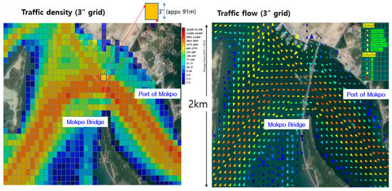
Figure 13.
Visualization of traffic density and traffic flow (close view, ~2 km: Mokpo bridge and Port of Mokpo area).
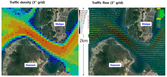
Figure 14.
Visualization of traffic density and traffic flow (close view, ~2 km: Port of Mokpo approach).
The directions of inbound and outbound vessels were clearly distinguished in the flow diagram. The arrows were generally long and uniform, reflecting relatively high speeds and a linear route structure. However, in the vicinity of the channel junction, the arrow directions and lengths became irregular, indicating navigational variability caused by crossing and merging of vessel movements. These findings suggest that even within the same channel section, traffic patterns vary by location, reflecting the structural characteristics of entrance routes. By integrating density and flow, the results demonstrated that traffic characteristics in the study area can be explained not only by vessel passage frequency (density) but also by direction and speed. Even in high-density zones, different speed and directional distributions were observed, while in low-density zones, stable routes and relatively high-speed patterns were evident. These outcomes confirm that the proposed model serves as a useful tool for intuitively interpreting dynamic traffic structure. Furthermore, the model holds practical and policy-oriented potential for supporting route decision-making for MASS, managing ports and narrow channels, predicting congestion, and assessing navigational risks.
4. Discussion & Conclusions
The high-resolution traffic model proposed in this study exhibits several distinctive features compared with conventional density-based marine traffic analyses. Previous studies have typically calculated grid-based traffic density from AIS data and represented it through color-coded heatmaps. While such approaches are useful for intuitively identifying zones of concentrated traffic zones, limitations are evident as they are not able to capture dynamic characteristics such as vessel direction and speed. However, the same AIS data were applied to high-resolution grids of approximately 90 m in this study, and both direction and speed calculated for each grid cell were visualized using arrow symbols. This approach clearly revealed the dynamic traffic structure that was difficult to discern from traditional analyses.
The main contributions of this study are summarized as follows:
- Proposal of a traffic flow visualization model: A traffic flow diagram was designed so that it integrates density, average speed, and dominant direction within each grid cell into a single arrow symbol.
- Application of high-resolution grids: The study area was divided into grid cells of approximately 90 m × 90 m.
- Analysis of Mokpo coastal data: AIS data from 2022–2023 were used to visualize traffic characteristics in major zones, including port approaches, narrow channels, and offshore routes.
- Visualization results: Traffic density maps and flow diagrams were presented to compare and analyze density, direction, and speed distributions across different zones of the study area.
As summarized in Table 3, these features highlight clear distinctions of the proposed model compared with traditional density-based models. Whereas conventional models are limited to describing the spatial concentration of traffic, the proposed model incorporates direction and speed in addition to density, thereby enabling more detailed and precise interpretation of maritime traffic structures.
Table 3.
Comparison between conventional density-based models and the proposed traffic flow visualization model.
Nevertheless, this study has several limitations. First, the analysis was limited to the coastal waters of Mokpo, so further applications to different sea areas and diverse traffic environments are required to verify the generalizability of the proposed model. However, the proposed traffic flow visualization model is not limited to the study area and can be applied to other maritime regions with different traffic characteristics, as its structure is based on universally available AIS-derived variables such as vessel position, speed, and direction.
Second, the study relied on post-processing of historical AIS data and has not yet been linked to a real-time data processing and visualization system. Nevertheless, the proposed traffic flow visualization model has the potential to be adapted for real-time data streams. Unlike accumulated historical analysis, real-time traffic modeling requires additional considerations such as computational efficiency, rapid data processing, and the immediate incorporation of dynamic changes in vessel movements. Therefore, methodological improvements and structural modifications of the current model would be necessary to make it suitable for live applications. Based on expert consultations, the demand for real-time traffic flow models has been strongly recognized, and our research team plans to address this as one of the main research directions.
In addition, the model structure can be flexibly adapted to different temporal resolutions, which allows for the examination of short-term variations in traffic flow, such as differences between morning and afternoon periods or seasonal patterns. Future research will therefore focus on identifying the optimal combination of grid size and time intervals to support both macroscopic, long-term analyses and dynamic, short-term monitoring required for autonomous navigation and smart port operations. Integrating real-time data acquisition and processing with the proposed model would further enable its development into a practical tool for immediate use in VTS operations and MASS navigation support.
Lastly, although the present study proposed a dynamic traffic flow model integrating density, direction, and speed, it did not directly address the concept of critical capacity in maritime waterways. In conventional marine traffic research, critical capacity is defined as the maximum traffic volume that can safely pass through a specific area at a given speed, which requires consideration of vessel dimensions and occupied surface area. While several studies have examined critical capacity from this perspective, current density-based marine traffic models, including those reviewed in this paper, primarily rely on the number of vessel passages per unit area and time. As a result, the relationship between traffic density, traffic flow, and critical capacity remains insufficiently explored in maritime contexts.
Future research should therefore aim to establish a theoretical linkage between these variables to support more effective traffic control and management strategies. Incorporating vessel size, occupied area, and flow capacity parameters into the proposed model would enable quantitative assessment of waterway efficiency and safety under varying traffic conditions.
Author Contributions
D.H.O. and N.I.; methodology, D.H.O., N.I. and F.Z.; software, D.H.O., N.I. and F.Z.; validation, D.H.O. and N.I.; formal analysis, D.H.O. and N.I.; investigation, D.H.O. and N.I.; resources, D.H.O. and N.I.; data curation, D.H.O. and F.Z.; writing—original draft preparation, D.H.O.; writing—review and editing, visualization, N.I.; supervision, N.I.; project administration, N.I.; funding acquisition, N.I. All authors have read and agreed to the published version of the manuscript.
Funding
This research was supported by the Korea Institute of Marine Science and Technology Promotion (KIMST), funded by the Ministry of Oceans and Fisheries (RS-2023-00238653).
Data Availability Statement
All data and materials are available on request from the corresponding author. The data are not publicly available due to ongoing research using a part of the data.
Conflicts of Interest
The authors declare no conflicts of interest.
Abbreviations
The following abbreviations are used in this manuscript:
| MASS | Maritime Autonomous Surface Ships |
| VTS | Vessel Traffic Services |
| AIS | Automatic Identification System |
| LOA | Length overall |
| SOG | Speed Over Ground |
| PSO | Particle Swarm Optimization |
| DBSCAN | Density-Based Spatial Clustering of Applications with Noise |
| Soft-DTW | Soft Dynamic Time Warping |
| CNN-LSTM-SE | Convolutional Neural Network–Long Short-Term Memory with Squeeze-and-Excitation |
| SOLAS | International Convention for the Safety of Life at Sea |
| MMSI | Maritime Mobile Service Identity |
| IMO | International Maritime Organization |
| UTC | Coordinated Universal Time |
| COG | Course Over Ground |
| ETA | Estimated Time of Arrival |
| RGB | Red–Green–Blue (color model) |
| kts | knots (nautical miles per hour) |
| COLREGs | Convention on the International Regulations for Preventing Collisions at Sea, 1972 |
References
- Sanchez-Gonzalez, P.-L.; Díaz-Gutiérrez, D.; Leo, T.J.; Núñez-Rivas, L.R. Toward Digitalization of Maritime Transport? Sensors 2019, 19, 926. [Google Scholar] [CrossRef]
- Yildiz, S.; Uğurlu, Ö.; Loughney, S.; Wang, J.; Tonoğlu, F. Spatial and statistical analysis of operational conditions influencing accident formation in narrow waterways: A Case Study of Istanbul Strait and Dover Strait. Ocean. Eng. 2022, 265, 112647. [Google Scholar] [CrossRef]
- Issa, M.; Ilinca, A.; Ibrahim, H.; Rizk, P. Maritime Autonomous Surface Ships: Problems and Challenges Facing the Regulatory Process. Sustainability 2022, 14, 15630. [Google Scholar] [CrossRef]
- Alamoush, A.S.; Ölçer, A.I.; Ballini, F. Drivers, opportunities, and barriers, for adoption of Maritime Autonomous Surface Ships (MASS). J. Int. Marit. Saf. Environ. Aff. Shipp. 2024, 8, 2411183. [Google Scholar] [CrossRef]
- Homayouni, S.M.; Pinho de Sousa, J.; Moreira Marques, C. Unlocking the potential of digital twins to achieve sustainability in seaports: The state of practice and future outlook. WMU J. Marit. Aff. 2025, 24, 59–98. [Google Scholar] [CrossRef]
- Wang, K.; Liang, M.; Li, Y.; Liu, J.; Liu, R.W. Maritime Traffic Data Visualization: A Brief Review. In Proceedings of the 2019 IEEE 4th International Conference on Big Data Analytics (ICBDA), Suzhou, China, 15–18 March 2019; pp. 67–72. [Google Scholar] [CrossRef]
- Wolsing, K.; Roepert, L.; Bauer, J.; Wehrle, K. Anomaly Detection in Maritime AIS Tracks: A Review of Recent Approaches. J. Mar. Sci. Eng. 2022, 10, 112. [Google Scholar] [CrossRef]
- Kim, H.-S.; Lee, E.; Lee, E.-J.; Hyun, J.-W.; Gong, I.-Y.; Kim, K.; Lee, Y.-S. A Study on Grid-Cell-Type Maritime Traffic Distribution Analysis Based on AIS Data for Establishing a Coastal Maritime Transportation Network. J. Mar. Sci. Eng. 2023, 11, 354. [Google Scholar] [CrossRef]
- Son, W.-J.; Kim, H.-C.; Lee, J.-S.; Cho, I.-S. Analysis of Extraction Method for Maritime Traffic Intensity Zone Through Occupancy Rate of Automatic Identification System Data. IEEE Access 2024, 12, 92718–92732. [Google Scholar] [CrossRef]
- Son, W.-J.; Cho, I.-S. Optimal maritime traffic width for passing offshore wind farms based on ship collision probability. Ocean. Eng. 2024, 313, 119498. [Google Scholar] [CrossRef]
- Yang, Y.; Liu, Y.; Li, G.; Zhang, Z.; Liu, Y. Harnessing the power of Machine learning for AIS Data-Driven maritime Research: A comprehensive review. Transp. Res. Part E Logist. Transp. Rev. 2024, 183, 103426. [Google Scholar] [CrossRef]
- Kim, Y.-J.; Lee, J.-S.; Pititto, A.; Falco, L.; Lee, M.-S.; Yoon, K.-K.; Cho, I.-S. Maritime Traffic Evaluation Using Spatial-Temporal Density Analysis Based on Big AIS Data. Appl. Sci. 2022, 12, 11246. [Google Scholar] [CrossRef]
- Lee, D.; Jang, D.; Yoo, S. Development of a Multidimensional Analysis and Integrated Visualization Method for Maritime Traffic Behaviors Using DBSCAN-Based Dynamic Clustering. Appl. Sci. 2025, 15, 529. [Google Scholar] [CrossRef]
- Son, J.-H.; Shin, O.-K.; Park, H.-C. Ship Route Pattern Extraction from AIS Data: Based on PSO Algorithm. J. Korean Inst. Inf. Technol. 2022, 20, 27–34. [Google Scholar] [CrossRef]
- Huang, C.; Qi, X.; Zheng, J.; Zhu, R.; Shen, J. A maritime traffic route extraction method based on density-based spatial clustering of applications with noise for multi-dimensional data. Ocean. Eng. 2023, 268, 113036. [Google Scholar] [CrossRef]
- Liu, D.; Rong, H.; Guedes Soares, C. Shipping route modelling of AIS maritime traffic data at the approach to ports. Ocean. Eng. 2023, 289, 115868. [Google Scholar] [CrossRef]
- Luong, T.N.; Hwang, S.; Im, N. Harbour Traffic Hazard Map for real-time assessing waterway risk using Marine Traffic Hazard Index. Ocean. Eng. 2021, 239, 109884. [Google Scholar] [CrossRef]
- Sui, Z.; Wang, S.; Wen, Y.; Cheng, X.; Theotokatos, G. Multi-state ship traffic flow analysis using data-driven method and visibility graph. Ocean. Eng. 2024, 298, 117087. [Google Scholar] [CrossRef]
- Wang, X.; Xiao, Y. A Deep Learning Model for Ship Trajectory Prediction Using Automatic Identification System (AIS) Data. Information 2023, 14, 212. [Google Scholar] [CrossRef]
- Wang, J.; Wang, X.; Zhou, J. Model selection for predicting marine traffic flow in coastal waterways using deep learning methods. Ocean. Eng. 2025, 329, 121151. [Google Scholar] [CrossRef]
- Zaman, U.; Khan, J.; Lee, E.; Balobaid, A.S.; Aburasain, R.Y.; Kim, K. Deep learning innovations in South Korean maritime navigation: Enhancing vessel trajectories prediction with AIS data. PLoS ONE 2024, 19, e0310385. [Google Scholar] [CrossRef]
- Zhang, B.; Hirayama, K.; Ren, H.; Wang, D.; Li, H. Ship Anomalous Behavior Detection Using Clustering and Deep Recurrent Neural Network. J. Mar. Sci. Eng. 2023, 11, 763. [Google Scholar] [CrossRef]
- Kim, K.I.; Park, G.K.; Jeong, J.S. Analysis of marine accident probability in Mokpo waterways. J. Navig. Port Res. 2011, 35, 729–733. [Google Scholar] [CrossRef]
- Hall, F.L. Traffic Stream Characteristics; Federal Highway Administration (FHWA); U.S. Department of Transportation: Washington, DC, USA, 1996. Available online: https://www.fhwa.dot.gov/publications/research/operations/tft/chap2.pdf (accessed on 3 October 2025).
- Li, J.; Zhang, H.M. Fundamental diagram of traffic flow. Transp. Res. Rec. J. Transp. Res. Board 2011, 2260, 50–59. [Google Scholar] [CrossRef]
- Milojević, S. Power law distributions in information science: Making the case for logarithmic binning. J. Am. Soc. Inf. Sci. Technol. 2010, 61, 2417–2425. [Google Scholar] [CrossRef]
- Jiang, D.; Shi, G.; Ma, L.; Li, W.; Wang, X.; Zhu, G. A Dynamic Trajectory Temporal Density Model for Analyzing Maritime Traffic Patterns. J. Mar. Sci. Eng. 2025, 13, 381. [Google Scholar] [CrossRef]
- Huang, Y.; Yip, T.L.; Wen, Y. Comparative analysis of marine traffic flow in classical models. Ocean. Eng. 2019, 187, 106195. [Google Scholar] [CrossRef]
Disclaimer/Publisher’s Note: The statements, opinions and data contained in all publications are solely those of the individual author(s) and contributor(s) and not of MDPI and/or the editor(s). MDPI and/or the editor(s) disclaim responsibility for any injury to people or property resulting from any ideas, methods, instructions or products referred to in the content. |
© 2025 by the authors. Licensee MDPI, Basel, Switzerland. This article is an open access article distributed under the terms and conditions of the Creative Commons Attribution (CC BY) license (https://creativecommons.org/licenses/by/4.0/).