Article

Real-Time Digital Twin for Structural Health Monitoring of Floating Offshore Wind Turbines

by
Andres Pastor-Sanchez
1,2,*,
Julio Garcia-Espinosa
1,2,*,
Daniel Di Capua
2,3,
Borja Servan-Camas
2 and
Irene Berdugo-Parada
2
1
Departamento de Arquitectura, Construcción y Sistemas Oceánicos y Navales, Escuela Técnica Superior de Ingenieros Navales, Universidad Politécnica de Madrid (UPM), 28040 Madrid, Spain
2
Centre Internacional de Mètodes Numèrics en Enginyeria (CIMNE), Gran Capitan s/n, 08034 Barcelona, Spain
3
Departamento de Resistencia de Materiales y Estructuras a la Ingeniería (RMEE), Universidad Politécnica de Cataluña (UPC), 08019 Barcelona, Spain
*
Authors to whom correspondence should be addressed.
J. Mar. Sci. Eng. 2025, 13(10), 1953; https://doi.org/10.3390/jmse13101953
Submission received: 11 September 2025 / Revised: 3 October 2025 / Accepted: 8 October 2025 / Published: 12 October 2025
(This article belongs to the Section Ocean Engineering)

Abstract

Digital twins (DTs) offer significant promise for condition-based maintenance of floating offshore wind turbines (FOWTs); however, existing solutions typically compromise either on physical rigor or real-time computational performance. This paper presents a real-time DT framework that resolves this trade-off by embedding a hydro-elastic reduced-order model (ROM) that accurately captures structural dynamics and fluid–structure interaction. Integrated in a cloud-ready Internet of Things architecture, the ROM reconstructs full-field displacements, von Mises stresses, and fatigue metrics with near real-time responsiveness. Validation on the 5 MW OC4-DeepCWind semi-submersible platform shows that the ROM reproduces finite-element (FEM) displacements and stresses with relative errors below 1%. A three-hour load case is solved in 0.69 min for displacements and 3.81 min for stresses on a consumer-grade NVIDIA RTX 4070 Ti GPU—over two orders of magnitude faster than the full FEM model—while one million fatigue stress histories (1000 hotspots × 1000 operating scenarios) are processed in 37 min. This efficiency enables continuous structural monitoring, rapid *what-if* assessments and timely decision-making for targeted inspections and adaptive control. By effectively combining physics-based reduced-order modeling with high-throughput computation, the proposed framework overcomes key barriers to DT deployment: computational overhead, physical fidelity and scalability. Although demonstrated on a steel platform, the approach is readily extensible to composite structures and multi-turbine arrays, providing a robust foundation for cost-effective and reliable deep-water wind-energy operations.

1. Introduction

Offshore wind energy is becoming increasingly important in the global transition to renewables. To harness stronger and more consistent winds, the sector is moving beyond shallow-water fixed foundations and into deeper waters using floating platforms. However, turbines operating in these environments experience complex, coupled loads from variable winds, dynamic waves, and ocean currents. These conditions make it particularly challenging to assess structural integrity and monitor long-term health.
Digital twins (DTs)—virtual replicas of physical systems that evolve with real-time data—are emerging as essential tools for managing these challenges. Unlike DTs used primarily during the design phase, operational DTs provide continuous insight into the structural condition and fatigue state of key components. This is especially valuable for offshore platforms, where routine inspections are expensive and logistically difficult. By enabling early detection of damage and optimizing maintenance planning, DTs help extend turbine lifespan and reduce the levelized cost of energy (LCOE).
To better understand how DTs have been applied to offshore wind structures and identify remaining challenges, developments in the literature are reviewed. Complementary domain-specific reviews deepen these findings for floating systems and turbine subsystems, emphasizing physics-aware twins, sensor integration, and fatigue-relevant KPIs in operational settings [1,2].
In recent years, digital twin (DT) technology for offshore wind turbines has advanced significantly, with research spanning structural monitoring, drivetrain diagnostics, floating platform dynamics, and hybrid modeling strategies.
Several studies have addressed structural reliability and fatigue life prediction. Augustyn [3] developed a DT framework for updating substructure reliability using monitoring data, while Jorgensen [4] incorporated uncertainty propagation through Gaussian Process surrogates to assess fatigue life. These works highlight the value of DTs in risk-informed maintenance planning, although they remain focused on offline or probabilistic evaluations rather than operational deployment. Building on this, recent work has addressed environmental dependence and data scarcity in fatigue assessment for FOWTs: Yu & Xu quantify fatigue reliability under correlated wind–wave–current loads, while Gaidai et al. propose a deconvolution-extrapolation strategy that improves long-term fatigue estimates from limited records [5,6].
Efforts targeting drivetrain and internal components have explored predictive capabilities. Moghadam [7] proposed a torsional dynamic model for gearbox health monitoring in floating wind turbines, and Mehlan [8] used virtual sensing to estimate loads and fatigue in uninstrumented drivetrain areas. While both approaches offer subsystem-level insights, they lack full-structure integration and real-time feedback.
For floating platforms and mooring systems, Walker [9] developed a DT to estimate mooring-line tensions, validated using operational data from Hywind Scotland. In a more comprehensive approach, Branlard [10] demonstrated a physics-based DT validated on the full-scale TetraSpar platform, achieving fatigue estimates within 10–15% of measured values. These examples highlight a shift toward higher-fidelity structural models, but also underscore the computational demands of such implementations.
These application-level advances are complemented by survey evidence that FOWT-focused DTs remain bottlenecked by real-time coupled modeling and credible fatigue pipelines—precisely the gaps highlighted in recent floating-wind DT reviews [1].
Real-world deployments of structural DTs remain relatively limited. Although several open-source initiatives have emerged, they frequently depend on simplified models or external simulation engines, which restrict their predictive fidelity.
Beyond application-specific developments, recent studies have explored novel methodological frameworks. Bull [11] introduced a probabilistic DT architecture based on multiple candidate models, while Mousavi [12] proposed a hybrid strategy that combines physics-based simulation with deep learning for damage detection. These approaches aim to balance interpretability with computational efficiency but are rarely validated in real-time or offshore contexts. In parallel, reduced-order modeling continues to expand toward non-linear regimes: Simpson et al. demonstrate a data-driven AE-LSTM ROM for monopile dynamics achieving 300 × speed-ups while retaining predictive fidelity, illustrating how non-linear surrogates can be plugged into DT pipelines without sacrificing response quality [13].
Finally, recent reviews [14,15,16] have synthesized these contributions, pointing to persistent challenges: limited real-time capabilities, high computational cost, and a lack of scalable, physically grounded models. These gaps motivate the development of digital twins that integrate efficient simulation with real-time sensor data, particularly for floating offshore wind turbines, where dynamic loads and remote operation heighten the need for advanced monitoring solutions. Recent wind-specific syntheses echo these themes for both floating platforms and component-level twins, calling for transparent physics, uncertainty-aware fatigue evaluation, and robust real-time data plumbing [1,2].
A notable step toward operational deployment is the open-source platform introduced by Pacheco-Blázquez [17], which combines real-time sensing, automated remaining-useful-life estimation, and cloud-based visualization for composite offshore structures. Owing to its modular, publicly available architecture, this platform is adopted and further extended in the present work as the technological backbone of the proposed structural Digital Twin.
Despite recent progress, developing effective digital twins (DTs) for offshore wind turbines remains challenging. Many current solutions rely heavily on data-driven models, such as deep learning, which often struggle to generalize beyond their training data and lack interpretability grounded in physical principles. This issue is particularly relevant in offshore environments, where access to high-quality, long-term monitoring data is limited. In contrast, physics-based methods—like Integrated Load Analysis (ILA)—offer a reliable and transparent foundation but come with high computational costs, making them impractical for real-time use.
These limitations point to a clear need: a digital twin that balances physical fidelity with real-time performance.
To address this, a real-time Digital Twin framework is presented, specifically designed for the unique demands of floating offshore wind turbines. The framework integrates three main components: (1) an Internet of Things (IoT) platform that streams and manages sensor data from both the environment and the turbine; (2) a reduced-order aero-servo-hydro-elastic model (ROM) obtained from a tightly coupled, time-domain finite-element solver; the ROM keeps the main structural modes and supplies modal response-amplitude operators (MRAOs)—transfer functions that turn hydrodynamic, aerodynamic, control and mooring loads into their associated generalized modal coordinates Servan-Camas & García-Espinosa [18,19,20]; (3) a Python-based engine that uses the ROM results to compute critical structural responses—such as displacements, stresses, and fatigue indicators—in real time. Together, these elements enable fast, scalable, and accurate structural monitoring, supporting condition-based maintenance and informed operational decisions. This hybrid approach combines the interpretability of physics-based models with the responsiveness required for real-time monitoring—a capability not yet demonstrated in prior DT implementations for floating offshore wind turbines.
The paper is structured as follows: First, we present the methodological foundations, detailing the governing fluid–structure equations and the projection-based reduced-order modeling approach that underpins the fast structural solver. Next, we introduce the proposed real-time digital twin framework, detailing its architecture, hardware–software integration, reduced-order structural solver, and data-management strategies. Then, we validate the framework with the DeepCWind semi-submersible case study, assessing both accuracy and computational performance under realistic metocean conditions and illustrating the advantages for real-time structural health monitoring and predictive maintenance. Finally, we summarize the key contributions and implications of the research.

2. Literature Review

2.1. Background and Motivation

The global offshore wind sector is projected to reach 380 GW by 2030 and 2000 GW by 2050, according to IRENA and the Global Offshore Wind Alliance [21,22]. As the industry moves beyond shallow-water fixed foundations into depths exceeding 60 m, floating offshore wind turbines (FOWTs) benefit from stronger and more consistent winds—with offshore installations achieving capacity factors of 40–50% compared to typical onshore values around 35% [23]. However, these platforms face complex, coupled loads from variable winds, waves, and currents, significantly complicating structural integrity assessment.
Digital Twins (DTs)—virtual replicas that evolve with real-time data—are emerging as essential tools for managing these challenges. Unlike DTs used primarily during the design phase, operational DTs provide continuous insight into structural condition and fatigue state throughout the turbine’s life. This capability is particularly valuable offshore, where maintenance visits can cost upward of $20,000 per turbine for drone inspections alone, with major component repairs reaching hundreds of thousands of dollars [24]. By enabling early damage detection and optimizing maintenance, DTs can reduce the levelized cost of energy (LCOE) by 5–10% through improved operational efficiency and reduced downtime [25,26]. Complementary domain-specific reviews deepen these findings for floating systems and turbine subsystems, emphasizing physics-aware twins, sensor integration, and fatigue-relevant KPIs in operational settings [1,2].

2.2. Recent Advances

Digital twin technology for offshore wind has advanced across multiple domains. For structural reliability, Augustyn (2021) developed a framework for updating substructure reliability using monitoring data [3], while Jorgensen (2023) incorporated uncertainty propagation through Gaussian Process surrogates for fatigue assessment [4]. These works enable risk-informed maintenance but remain focused on offline or probabilistic evaluations rather than operational deployment. Addressing floating-specific challenges, Yu & Xu (2024) quantified fatigue under correlated wind–wave–current loads [5], while Gaidai et al. (2023) proposed strategies for long-term fatigue estimates from limited operational records [6].
Component monitoring has evolved through virtual sensing. Moghadam (2021) developed torsional models for gearbox health in FOWTs [7], while Mehlan (2022) estimated loads in uninstrumented drivetrain areas [8]. However, these approaches lack full-structure integration and real-time feedback capabilities.
For floating platforms, Walker (2022) created a DT for mooring-line tension estimation validated on Hywind Scotland [9]. Branlard (2024) demonstrated a comprehensive physics-based DT on the TetraSpar platform, achieving fatigue estimates within 10–15% of measurements [10]. These implementations highlight both the potential and computational demands of high-fidelity models.
Methodological innovations seek to balance accuracy with efficiency. Bull (2024) introduced probabilistic multi-model architectures [11], while Mousavi (2024) combined physics-based simulation with deep learning [12]. Notably, Simpson et al. (2023) demonstrated reduced-order modeling achieving approximately 300× computational speed-ups while maintaining predictive fidelity [13]—illustrating how surrogates can enable real-time monitoring without sacrificing response quality.
Recent syntheses identify persistent challenges: limited real-time capabilities, high computational costs, and lack of scalable, physically grounded models [14,15,16]. Survey evidence indicates that FOWT-focused DTs remain bottlenecked by real-time coupled modeling and credible fatigue assessment pipelines [1]. Pacheco-Blázquez (2024) addressed some gaps with an open-source platform combining real-time sensing and cloud visualization, owing to its modular, publicly available architecture [17], providing a foundation we extend in this work.

2.3. Research Gap and Proposed Solution

Despite advances, a critical gap remains: existing solutions rely either on data-driven models lacking physical interpretability or on physics-based methods like Integrated Load Analysis that require computational resources incompatible with real-time operation. This dichotomy is particularly problematic offshore, where monitoring data is limited yet physically grounded predictions are essential for safety-critical decisions.
To address this, we present a real-time digital twin framework specifically for FOWTs that bridges physical fidelity and computational efficiency through three components:
  • IoT Infrastructure: A scalable platform streaming sensor data from both environmental and turbine systems, handling high-frequency measurements with quality assurance and anomaly detection.
  • Physics-Based ROM: A reduced-order aero-servo-hydro-elastic model derived from a tightly coupled, time-domain finite-element solver, retaining primary structural modes while providing modal response-amplitude operators (MRAOs). These transfer functions, based on the methodology of Servan-Camas & García-Espinosa (2023, 2025), efficiently map hydrodynamic, aerodynamic, control, and mooring loads to generalized modal coordinates [18,19].
  • Real-Time Engine: A Python-based processor computing critical responses— displacements, stresses, and fatigue indicators—with update rates suitable for operational decision support.
This hybrid approach uniquely combines physics-based reliability with real-time performance, building upon and extending Pacheco-Blázquez’s open-source framework [17] to provide practical condition-based maintenance capabilities not yet demonstrated in prior DT implementations for FOWTs.

2.4. Paper Organization

Section 3 presents the governing equations and projection-based reduced-order modeling approach. Section 4 details the digital twin architecture, hardware–software integration, and data management strategies. Section 5 validates the framework using the DeepCWind semi-submersible case study under realistic metocean conditions. Section 6 summarizes contributions and implications for the offshore wind industry.

3. Methodology

This section describes the implemented computational model for aero-servo-hydro-elastic analysis of floating offshore wind turbines.

3.1. Seakeeping Governing Equations

Assuming an inviscid, incompressible, and irrotational fluid domain Ω , the flow is represented by a velocity potential ϕ ( x , t ) that satisfies Laplace’s equation:
2 ϕ = 0 in Ω .
Appropriate boundary conditions are imposed on the free surface, the structure, and the seabed:
  • Free Surface ( Γ F S ): On the free surface with elevation ξ ( x , t ) , two conditions hold:
    • A kinematic condition ensuring that the free surface moves with the fluid:
      ξ t + ( U + h ϕ ) · h ξ = ϕ z .
    • A dynamic condition (from Bernoulli’s equation) that balances the pressure:
      ϕ t + U · h ϕ + 1 2 | h ϕ | 2 + g ξ = p f s ,
      where g is gravitational acceleration and p f s is the free surface pressure.
  • Body Surface ( Γ B ): On the wetted surface of the structure, a no-penetration condition is imposed:
    v ϕ · n = v p · n ,
    where v ϕ = ϕ is the fluid velocity, v p = u ˙ is the body velocity, and n is the unit normal.
  • Seabed ( Γ S ): At the rigid seabed, the no-penetration condition is as follows:
    v ϕ · n = 0 .
The pressure field is obtained from the unsteady Bernoulli equation. For example, at vertical coordinate z, the pressure is as follows:
P ( z ) = ρ g z ρ ϕ t + U · ϕ + 1 2 | ϕ | 2 ,
where ρ is the fluid density.
Solution decomposition: It is convenient to split the flow into an incident wave field and a disturbance due to the body. The solution is expressed as follows:
ϕ = ψ + ϕ and ξ = ζ + η ,
where ( ψ , ζ ) describe the incident waves and ( ϕ , η ) the diffracted components. Substituting into the governing equations yields a linear system (via a finite-element discretization) for ϕ [20]:
L ϕ = b B + b ζ 0 + b S ,
with L the discretized Laplace operator, and b terms representing boundary contributions. It is important to note that, in this work, the seakeeping problem is solved in the time domain using a finite-element method (FEM), thereby allowing straightforward coupling with the structural problem (see, e.g., [20,27]).

3.2. Fluid–Structure Governing Equations

Floating structures subject to wave loads experience dynamic fluid forces inducing structural responses. Under the assumption of small deformations, the linear elastic model in the structural domain Ω s is as follows:
· σ + b = ρ s u ¨ in Ω s ,
where u ( x , t ) is the displacement field, σ is the Cauchy stress tensor (linearly related to strain via Hooke’s law), b represents body forces (e.g., gravity), and ρ s is the material density.
Structural boundary conditions. On boundaries that are not in contact with the fluid, we impose the following:
  • Surface tractions on S σ : external pressures from waves or wind are applied as traction loads, σ n s = p n s , over the wetted hull and the exposed tower walls,
  • Point loads at the hub: the linearized aerodynamic model supplies a resultant force F hub and moment M hub acting at the end of a rigid bar that represents the rotor axis; these are assembled directly into the global load vector,
  • Mooring-line reactions: linearized mooring forces F m (Equation (17)) act at the fairlead attachment points.
Semi-discrete dynamic equilibrium. After a standard finite-element discretization of the structural weak form, the nodal displacements satisfy the second-order system [28]
M u ¨ + C u ˙ + K u = F ( t ) ,
where M , C , and K are the global mass, damping, and stiffness matrices and F ( t ) collects the time-dependent fluid-pressure loads acting on Γ F S I .
The damping matrix is taken as Rayleigh (proportional) damping,
C = α M + β K ,
with coefficients α and β chosen to reproduce the target modal damping ratios.
Fluid–Structure Coupling: At the interface Γ F S I , two conditions ensure proper coupling:
  • Pressure (stress) continuity: The fluid pressure p ϕ and structural stress must satisfy the following:
    σ · n s = p ϕ n s ,
    where n s is the normal from the solid (with n f = n s from the fluid).
  • Kinematic (no-penetration) continuity: The structural normal velocity equals the fluid particle velocity:
    u ˙ · n s = ϕ · n f .
These conditions allow the fluid pressure to act as a time-dependent load on the structure while the structural motion updates the fluid boundary.
In this work a partitioned, tightly coupled (two-way) strategy [27] is adopted to solve the hydro-elastic problem. Both the seakeeping and structural domains are discretized with the FEM, but the meshes need not conform at the common interface Γ B . Spatial transfer of data is performed with linear interpolation operators that map pressures from the fluid mesh to the structural mesh, and displacements in the opposite direction:
p S , Γ B = I F S p F , Γ B ,
u F , Γ B = I S F u S , Γ B ,
where p F , Γ B and u F , Γ B are the nodal fluid pressures and interface displacements on the fluid mesh, p S , Γ B and u S , Γ B are their counterparts on the structural mesh, and I F S , I S F are the corresponding interpolation matrices assembled once during preprocessing.

3.3. Aerodynamic and Mooring Linear Models

In addition to the hydro-elastic formulation described above, the reduced-order model incorporates linear representations of the aerodynamic rotor loads and the mooring-line restoring forces so that all external actions can be superposed consistently in the time domain.
Linearized rotor aerodynamics. Let ( x 0 , x ˙ 0 ) denote the steady operating point of the hub and define the small perturbations δ x = x x 0 and δ x ˙ = x ˙ x ˙ 0 . A first-order Taylor expansion of the non-linear aerodynamic load vector about that point yields
F a ( t ) F a 0 + M a δ x ¨ + B a δ x ˙ + K a δ x + C a δ u ,
where F a 0 is the mean rotor load, δ u collects small variations in the control inputs (blade pitch, generator torque, etc.), and M a , B a , K a and C a are the added-mass, aerodynamic damping, stiffness, and control-gain matrices obtained with the linearization tools available in OpenFAST [29].
Linearized mooring system. The quasi-static catenary mooring model is linearized in an analogous way about the equilibrium offset of the platform, giving
F m ( t ) F m 0 + M m δ x ¨ + B m δ x ˙ + K m δ x ,
where F m 0 is the static pretension and M m , B m , K m are the inertia, damping and stiffness matrices of the linearized mooring-line assembly.
Applicability of the linearized terms. Equations (16) and (17) involve linearizations of the aerodynamic and mooring contributions, and are therefore valid for small perturbations around representative operating points where the linearization assumptions hold.
The aerodynamic term in Equation (16) and the mooring term in Equation (17) are added to the modal right-hand side of Equation (21), preserving the real-time capability of the reduced-order model.

3.4. Real-Time Structural Solvers in SHM Digital Twins

In this work, the baseline structural formulation is a complete finite-element model of the platform substructure and tower with detailed geometry and properties, comprising up to several million degrees of freedom; we refer to this as the full-length model. Current full-length FEM-based structural dynamics models, integrating the coupled effects of wind, waves, and mooring loads in FOWTs, are too computationally demanding for real-time applications. Digital twins require fast yet accurate models, navigating a trade-off between simplicity and fidelity. Starting from the semi-discrete dynamic equilibrium in Equation (10), we construct a projection-based reduced-order model that retains high accuracy while enabling real-time performance.
Reduced-Order Modeling (ROM): ROMs reduce the number of degrees of freedom by focusing on the system’s dominant behavior. In this work, a Modal Matrix Reduction (MMR) approach is used. The full-order structural dynamics are described by Equation (10), with damping given by the Rayleigh model in Equation (11).
Natural vibration modes are determined from the eigenvalue problem:
( K ω i 2 M ) Φ i = 0 , i = 1 , 2 , , N ,
this eigenproblem yields real, positive eigenvalues ω i (the natural frequencies), each paired with a characteristic eigenvector (mode shape) Φ i . The structural displacement field can then be expanded as a linear combination of these eigenvectors [28]:
u ( t ) = i = 1 N q i ( t ) Φ i ,
where Q ( t ) = { q i ( t ) } i = 1 N are the modal generalized coordinates (modal amplitudes). In practice, only a much smaller subset of N m modes ( N m N ) is required to represent the structural response with sufficient accuracy. Retaining only these modes yield the following:
u ROM ( t ) = i = 1 N m q i ( t ) Φ i .
To ensure that the selection of modes is sufficient to accurately approximate the complete solution, we define ω cut ω N m max as the highest natural frequency kept in the truncated basis and impose ω cut 4 ω ˜ max , following Bathe [28].
Substituting Equation (20) into (10) and applying orthonormality yields N m decoupled modal equations:
q ¨ i ( t ) + 2 ζ i ω i q ˙ i ( t ) + ω i 2 q i ( t ) = f i ( t )
where f i ( t ) = Φ i T F ( t ) and ζ i is the damping ratio. Each modal equation is analogous to a damped single-degree-of-freedom oscillator.
For a floating platform, the global stiffness matrix K is positive semi-definite, so the eigenproblem above yields six zero (or near-zero) eigenvalues that correspond to rigid-body motions. The modal generalized coordinates therefore split naturally into two groups [28]:
Q R = { q 1 , q 2 , , q 6 } ,
Q D = { q 7 , q 8 , , q N m } ,
where Q R collects the six rigid-body modes and Q D the remaining flexible-body modes. The six independent Equation (22) associated with Q R are equivalent to the conventional rigid-body dynamics, which can be written in compact matrix form as
M RB u ¨ RB + B RB u ˙ RB + K RB u RB = F RB ,
where M RB , B RB , and K RB are the mass, damping, and hydrostatic restoring matrices associated with the rigid-body degrees of freedom; u RB comprises the three translational and three rotational components of the platform motion; F RB contains the integrated hydrodynamic, gravitational, and external forces and moments acting on the body.
Wave-induced MRAOs: To efficiently predict the response to wave excitation, the Modal Response Amplitude Operator (MRAO) is introduced. For a given mode m, the MRAO is defined as the ratio between the amplitude response of the mth mode and the amplitude of a monochromatic wave excitation of frequency ω ˜ and direction θ :
MRAO m ( ω ˜ , θ ) = χ m ( ω ˜ , θ ) H ( ω ˜ , θ )
where H ( ω ˜ , θ ) is the amplitude of the monochromatic wave excitation at ( ω ˜ , θ ) , and χ m ( ω ˜ , θ ) is the amplitude response of the mth mode.
The MRAOs are computed by performing simulations with white noise excitation in the domain, followed by a Fourier analysis to obtain the response amplitudes for the different frequencies.
Offshore wind turbines are subjected to broadband excitations. The wave field is characterized by a spectrum S ( ω ˜ ) (e.g., Pierson–Moskowitz or JONSWAP) and a directional spreading function D ( θ ) (satisfying D ( θ ) d θ = 1 ). Discretizing the spectrum into intervals Δ ω ˜ and Δ θ , each component is assigned an amplitude:
H ( ω ˜ , θ ) = 2 S ( ω ˜ ) D ( θ ) Δ ω ˜ .
A small random phase is applied to avoid perfect periodicity (i.e., ω ˜ is shifted to ω ˜ + δ ω ˜ , where δ ω ˜ is uniformly distributed in the range from Δ ω ˜ / 2 to + Δ ω ˜ / 2 ).
For a given wave spectrum S ( ω ˜ ) and directional discretization D ( θ ) , the wave contribution to the modal time history is reconstructed as
q m wave ( t ) = θ ω ˜ H ( ω ˜ , θ ) MRAO m ( ω ˜ , θ ) cos ω ˜ t + φ m ( ω ˜ , θ ) ,
Practical spectral/discretization settings. In routine operation, we resolve 0.125–12.5 Hz using piecewise-nonuniform binning (finer resolution around platform/tower resonances and control bandwidth, coarser elsewhere). Directional discretization every 10°. Each component uses independent random phase and small frequency jitter to avoid artificial periodicity. Amplitudes are normalized so the discretized spectrum reproduces target variance.
Wind-Induced MRAOs: For mode m, the wind Modal Response Amplitude Operator is defined as
MRAO m wind ( ω ˜ , ϕ ) = χ m wind ( ω ˜ , ϕ ) U ( ω ˜ , ϕ ) ,
where U ( ω ˜ , ϕ ) is the complex amplitude of the longitudinal wind–speed fluctuation with direction ϕ , and χ m wind is the resulting modal response. For a given turbulence spectrum U ( ω ˜ , ϕ ) and an appropriate directional discretization, the wind contribution to the modal time history is reconstructed as
q m wind ( t ) = ϕ ω ˜ U ( ω ˜ , ϕ ) MRAO m wind ( ω ˜ , ϕ ) cos ω ˜ t + φ m ( ω ˜ , ϕ ) ,
with random phase φ m added to prevent artificial periodicity. The total modal response used henceforth is the algebraic combination q m ( t ) = q m wave ( t ) + q m wind ( t ) .
A static offset q m static is added to account for steady loads, giving the total modal response:
q m total ( t ) = q m static + q m ( t ) .
To ensure the selected N m modes capture the significant dynamics, an energy-based selection is used. For mode m, define the vibrational energy as
E m = 1 2 ω m 2 q m 2 ( t ) ,
and choose N m such that
m = 1 N m E m 0.95 i = 1 N E i .
Figure 1 illustrates a typical modal energy distribution and the cumulative energy captured. In practice, even for detailed finite-element models of large floating turbines, retaining only a few hundred lowest-frequency modes is usually enough to surpass the 95% elastic-energy threshold defined in Equation (32) and to satisfy the cutoff criterion ω cut 4 ω ˜ max [28].
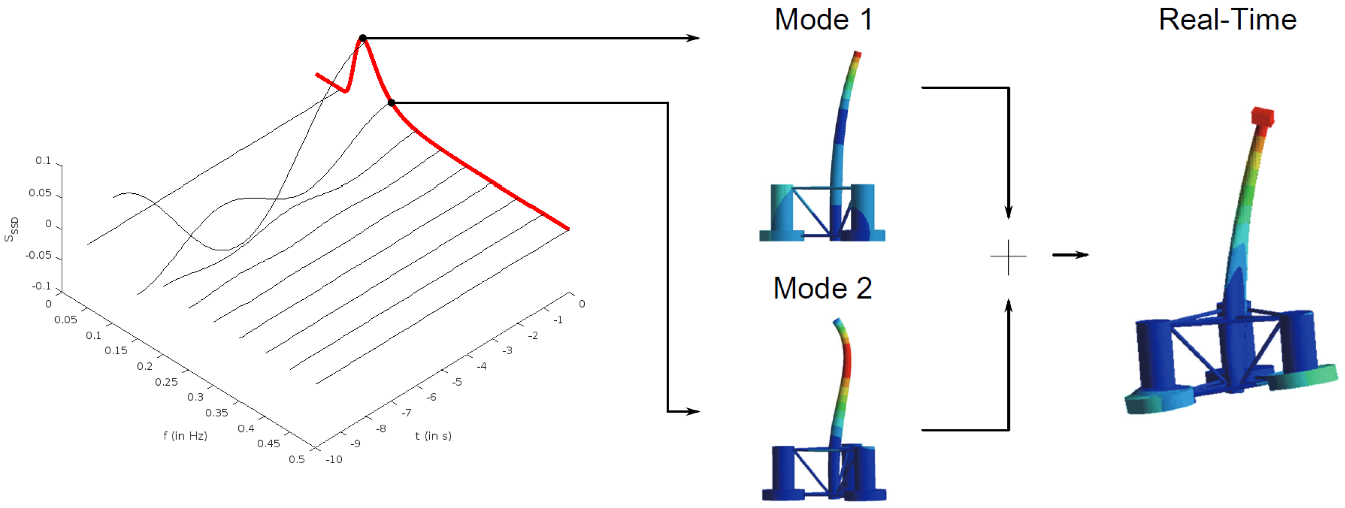
The displacement at a specific node and direction is reconstructed by summing the contributions of each mode, as illustrated in Figure 2:
u i , d ( t ) = m = 1 N m q m ( t ) [ Φ m ] i , d ,
where [ Φ m ] i , d represents the component of mode shape Φ m at node i in direction d, and q m ( t ) is the corresponding modal amplitude at time t.
This modal superposition approach allows the heavy offline computations (eigenmodes, MRAOs, spectral decomposition) to be precomputed. At runtime, updating the FOWT state becomes a fast summation over a small number of modes, enabling near real-time simulation.
Efficient Stress Calculation: Once u ( t ) is known, stresses are computed via the constitutive relation:
σ = D B u ,
where B is the strain–displacement matrix and D is the material matrix. Since B and D are constant for a given element in the linear regime, the product C = D B is precomputed for each element (and integration point). Thus, for each element with n nodes nodes:
σ ( g , t ) = i = 1 n nodes C ( i , g ) u i ( t ) ,
where g denotes the integration (Gauss) point. For shell elements with rotation dofs, the computation is split into membrane ( C m ) and bending ( C f ) contributions. The precomputed matrices C m and C f are obtained by Gauss-point integration of the matrix products D B m and D B f . Here, D is the constitutive (material) matrix and B m and B f are the membrane and bending strain–displacement matrices. The symbols w g denote the Gauss weights and n g p the number of Gauss points:
C m ( e ) = g = 1 n g p w g D B m ( e ) ( : , : , g ) , C f ( e ) = g = 1 n g p w g D B f ( e ) ( : , : , g ) .
σ top ( g , t ) = i C m ( i , g ) + t 2 C f ( i , g ) u i ( t ) ,
and similarly for σ bottom . This precomputation enables fast matrix–vector multiplications at each time step.
Although the validation case presented in Section 4 focuses on a steel structure, the same framework can be extended to other materials, including composites. By updating the stress recovery matrices to reflect the appropriate constitutive laws—such as anisotropic or layered stiffness models—the digital twin can accurately represent different material behaviors without requiring changes to the overall workflow.
Fatigue Evaluation: Fatigue analysis is performed in real time using the computed stress histories. First, the stress time series at critical locations is filtered to identify significant turning points (peaks and valleys) while ignoring minor fluctuations via a hysteresis filter. The 4-point Rainflow counting method (ASTM E1049-85 [30]) is then applied to these filtered signals to count stress cycles. Figure 3 illustrates the application of the Rainflow counting algorithm on a sample stress history. Cycle counts n i are obtained for each stress range, and fatigue damage is estimated using the Palmgren–Miner rule [31]:
D = i = 1 k n i N i ,
where N i is the fatigue life (from an S–N curve [32]) corresponding to the stress range in bin i. When D = 1 , the component’s fatigue life is fully consumed. Different S–N curves can be accommodated for various materials or components.
The ROM-based approach drastically reduces computational cost while preserving key dynamic features. Efficient stress recovery and real-time fatigue evaluation enable the digital twin to continuously monitor structural health and predict remaining useful life, which is crucial for proactive maintenance and operational decision-making.

4. Digital Twin for Structural Health Monitoring

IoT integration overview. The digital twin (DT) runs on the OSI4IOT microservices stack, which connects data sources to the physics-based ROM, storage, and visualization layers. The end-to-end data and control flow is summarized in Figure 4 and detailed in items 1–6 below.
  • Data ingestion: Sensors publish via MQTT (Mosquitto); forecasts fetched via OPeNDAP/HTTP on schedule.
  • Quality control: Node-RED flows perform gap filling, outlier filtering, resampling, and unit tagging.
  • Storage: Curated time series are written to TimescaleDB with asset/sensor metadata.
  • Compute: The Python (version 3.12) DT service subscribes to metocean/operational topics, generates spectra, runs the MRAO-based ROM, and computes displacements, stresses, and fatigue.
  • Publishing: Computed KPIs are written back to TimescaleDB (and optionally republished on MQTT).
  • Visualization and alerts: Grafana dashboards and the web 3D viewer render signals; thresholds trigger alarms.
Messages follow MQTT topics such as fowt/<asset>/sensors/<id> and fowt/ <asset>/dt/<kpi> (QoS 1), all time-stamped in UTC and resampled to a common Δ t to ensure alignment between raw and computed series. MQTT traffic is TLS-encrypted and broker access is authenticated; database access is role-based. Services scale independently (containerized) and stateless DT workers can be replicated for throughput.
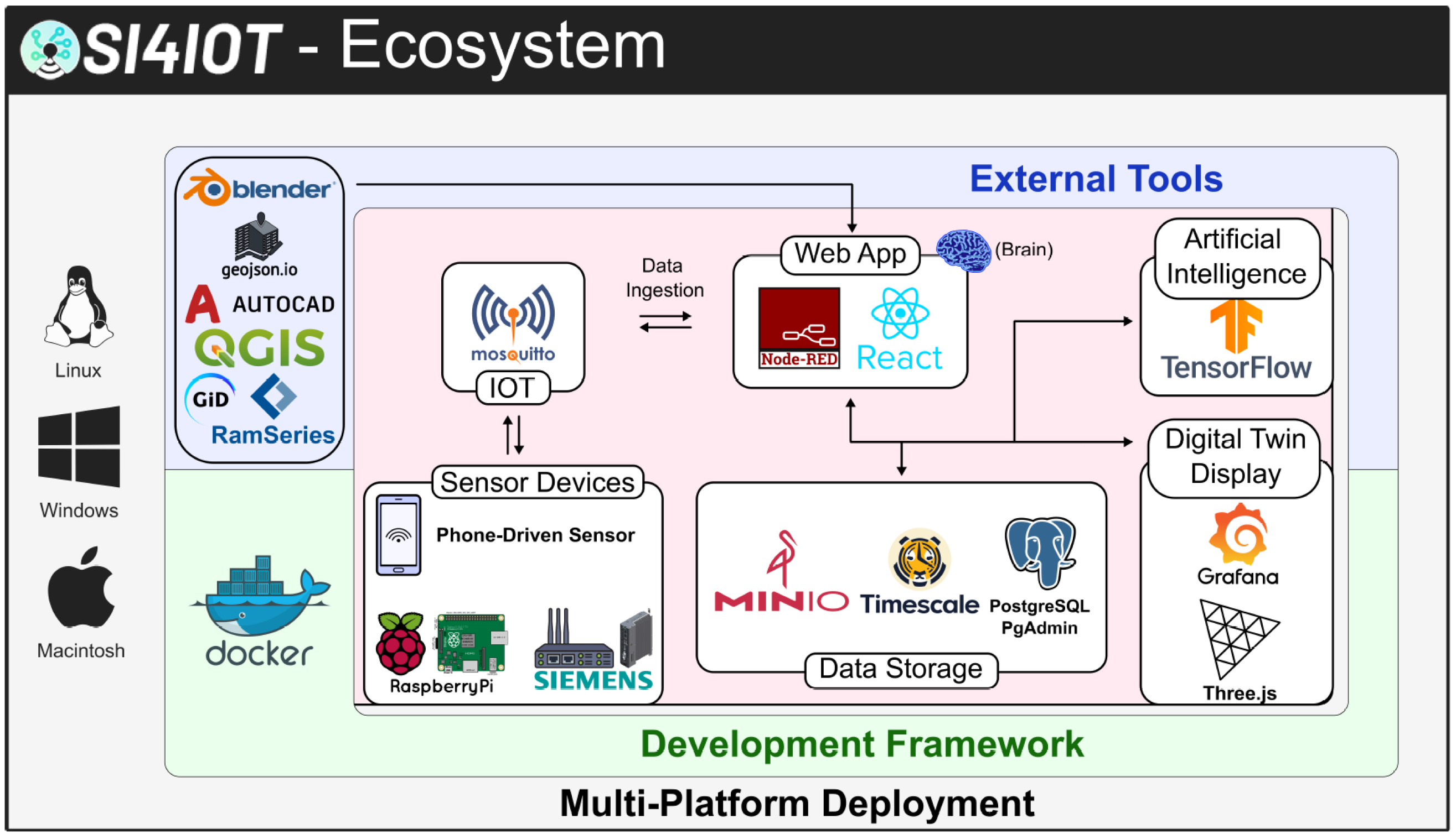
The OSI4IOT platform is built on a microservices architecture deployed through Docker containers, allowing each software component to be independently managed, scaled, and updated. The software stack is illustrated in Figure 5. A React-based frontend [34] provides the user interface, while data ingestion and processing are handled by automated workflows implemented in Node-RED [35]. Sensor data, whether from physical devices or virtual sources, are transmitted via the MQTT protocol, with message exchange coordinated by a Mosquitto broker [36]. This modular design enhances system robustness, facilitates fault isolation, and enables rapid adaptation to different deployment configurations.
Curated sensor and computed streams are stored in TimescaleDB [37] for high-throughput ingestion and sub-second queries, powering live Grafana dashboards [38], ROM-driven simulations, and alerting. Predictive analytics modules in PyTorch [39] are periodically retrained on historical data. Figure 6 shows an example dashboard with measured and computed indicators; panels refresh continuously from TimescaleDB, with role-based access and full time-stamped traceability.
In addition to real-time data visualization, the platform provides interactive 3D representations of the structural state. The 3D geometry and metadata of the digital twin are prepared through a dedicated visualization pipeline. Finite-element mesh data from RAMSeries [40]—including nodal coordinates, connectivity, and structural layout—are exported in JSON format and imported into Blender [41], where additional metadata are embedded (e.g., sensor locations, component IDs, animations). Blender then exports an enriched glTF model, which is loaded into the OSI4IOT platform for interactive web-based visualization. This workflow is illustrated in Figure 7.
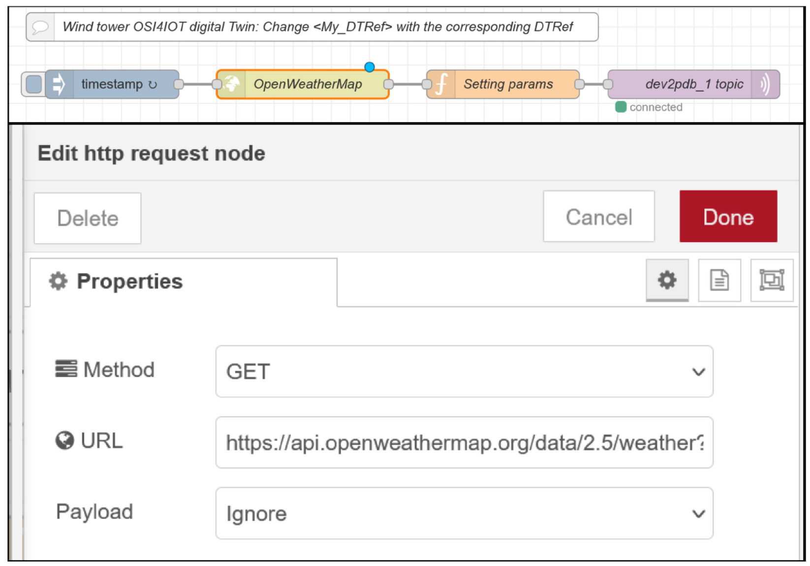
Beyond visualization, the DT integrates multi-source environmental inputs. Virtual sensors ingest external APIs such as OpenWeatherMap [42]; public datasets from Portus [43] and Copernicus [44] provide validated measurements and forecasts. Examples are shown in Figure 8 and Figure 9.
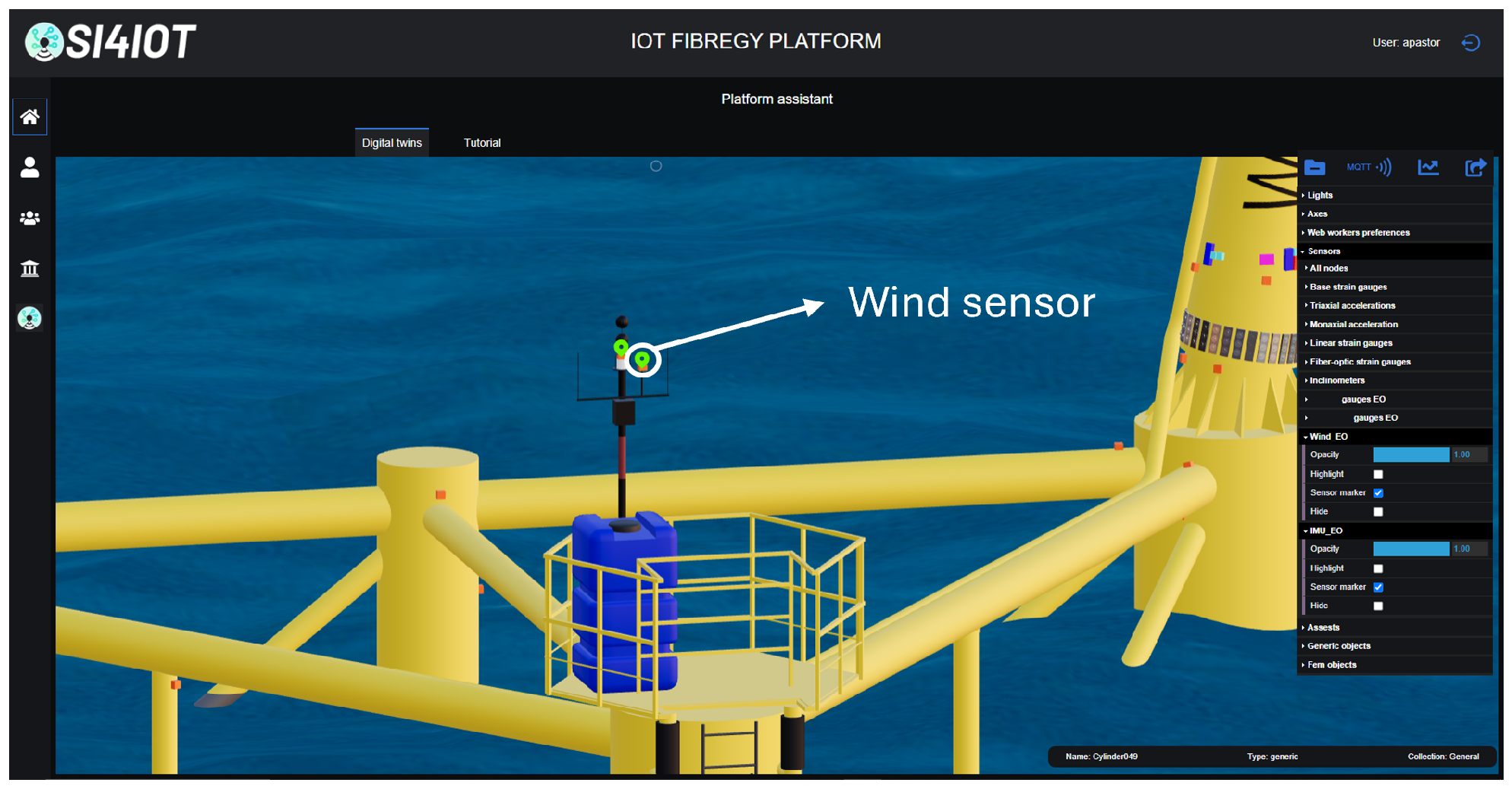
On-board instruments (e.g., anemometers and inertial measurement units, IMUs) complement remote sources with local, high-rate measurements (Figure 9).
All streams—virtual, public, and on-board—enter the platform via standard protocols: forecasts are fetched twice daily over OPeNDAP [47]; local sensors publish over MQTT. Signals are time-stamped and stored in TimescaleDB for monitoring and simulation. Prior to simulation, metocean series are quality-controlled (gap filling, outlier filtering, smoothing) and then converted into wave and wind spectra that drive the ROM described in Section 2.
This comprehensive data integration infrastructure enables hybrid monitoring strategies that combine local sensor measurements with remote data sources and virtual inputs. Real-time updates from physical instrumentation, simulation results, and predictive models are consolidated within a unified platform, providing a robust foundation for condition-based maintenance. The modular architecture ensures extensibility, allowing for seamless integration of additional sensor types, enhanced modeling capabilities, or large-scale deployment across multiple assets.

5. Case Study

To validate the proposed Digital Twin framework, the OC4–DeepCWind semi–submersible floating wind turbine (5 MW) [48] serves as the reference structure. The structural definition used here as the benchmark follows ServanCamas2025 [19]; Table 1 summarizes its principal characteristics. The assessment follows Bureau Veritas Design Load Case (DLC) 1.6 (Production) for an intact system stationed at Morro Bay (California), where the water depth is 200 m.
The metocean conditions considered fall into two groups:
(1)
Reference operating condition (RC)—used for the structural–response validation (displacements and stresses via ROM–FEM comparison). A hub–height mean wind speed U = 14.8 m s 1 is represented by an NPD spectrum (40 frequency components, 0.00027–2.8 Hz). The accompanying sea state is a unidirectional JONSWAP spectrum with significant height H s = 6 m and peak period T p = 14 s propagating from 0 ° . Currents are neglected.
(2)
Fatigue environmental conditions (FEC)—used for the hot-spot analysis. An array of 1000 metocean scenarios is generated by combining: wind speed U = 4 –25 m s−1 (5 discrete bins), significant wave height H s = 1 –8 m (4 bins), spectral peak period T p = 4 –20 s (5 bins), and wave incidence direction θ = 0 ° –330° (10 bins at 30° spacing). The Cartesian product of these bins ( 5 × 4 × 5 × 10 ) yields the 1000 distinct load cases employed to calculate fatigue damage at the selected hot-spot locations.
The finite element (FE) model contains 139,876 nodes and 315,417 triangular shell elements. With six degrees of freedom per node this yields 839,256 structural DOFs per time step, while stress at three Gauss points per element face and four stress components produces 7,570,008 evaluation points per step. A three hour simulation at 0.1 s resolution (108,000 steps) would therefore require roughly 9.1 × 10 10 displacement and 8.2 × 10 11 stress evaluations, far exceeding real-time capabilities.
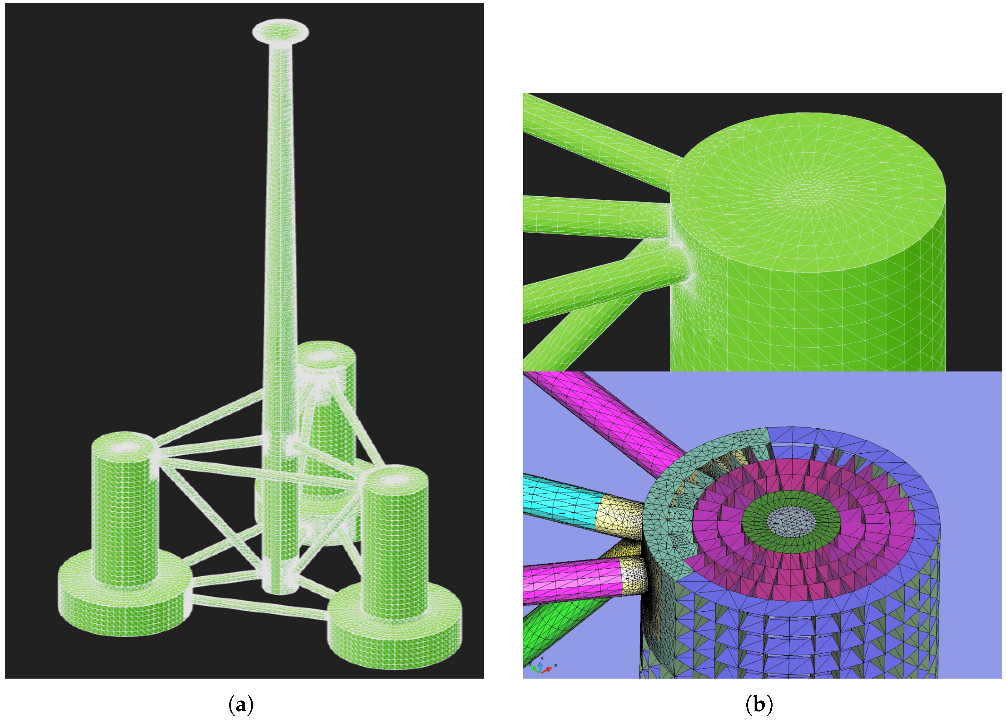
Figure 10a,b show the global FE mesh and a detailed view of the brace–column region, respectively. Figure 11 illustrates the deformation shape of a representative bending mode retained in the Reduced-Order Model (ROM).
Instead, the digital twin employs a projection-based Reduced-Order Model (ROM) built from the first 5006 vibration modes, whose highest retained natural frequency is 121 Hz, thereby reducing the computational burden by several orders of magnitude while preserving dynamic accuracy.

5.1. Structural Response

Displacements were computed using the reduced-order model (ROM) described in Section 2.3, which reconstructs the structural response from precomputed mode shapes and time-varying modal amplitudes driven by metocean loading under the reference condition. The ROM was validated against a full finite element model (FEM) of the OC4-DeepCWind platform to assess its accuracy and suitability for real-time integration in the digital twin.
Figure 12 illustrates a sample displacement output from the digital twin at a representative time step. This visualization, continuously updated as new environmental data arrive, enables real-time monitoring of platform and tower motion.
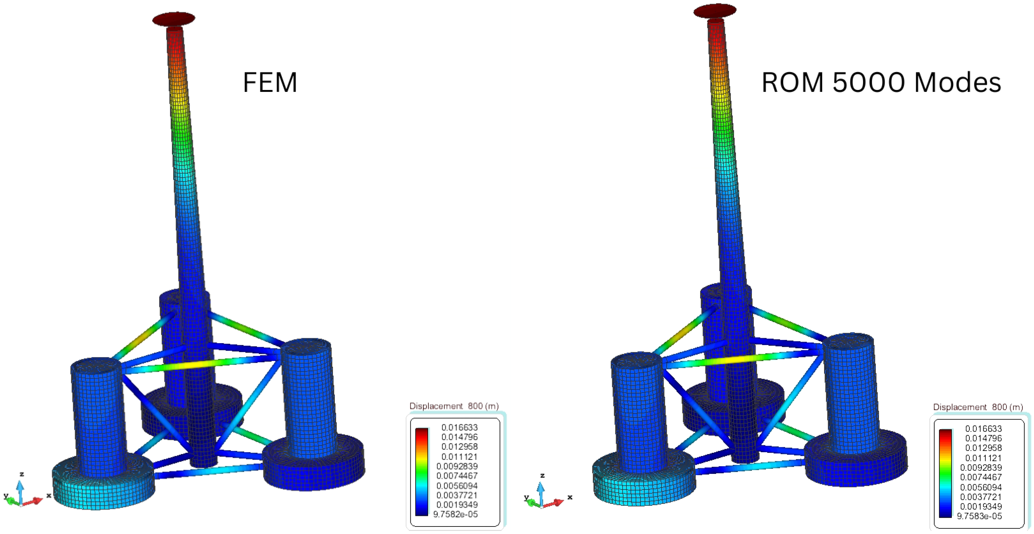
Global validation results are shown in Figure 13, comparing the displacement fields produced by the FEM and ROM at the same time step. The ROM accurately reproduces the full-field deformation, including high-gradient regions near the tower base and column–brace junctions, using only a fraction of the original degrees of freedom.
To examine local accuracy, the displacement time history at a critical node (located at a brace–column connection) was compared between models. Figure 14 shows both the node location and the time-series comparison. The ROM and FEM curves are visually indistinguishable, confirming that dynamic response features are fully preserved.
Quantitatively, the maximum absolute error across all nodes and time steps was below 10 8 m. The mean-squared error was 10 10 m2, with a root-mean-square error around 10 10 m. Even in high-motion regions, local errors remained below 10 9 m, and the maximum relative error for displacement was consistently under 1%. These results confirm that the ROM achieves FEM-level accuracy while remaining computationally efficient for real-time applications.

5.2. Stress

Once the displacement field is computed, the digital twin calculates the corresponding stress distribution using the recovery process described in Section 2.3 for the same reference condition. The von Mises equivalent stress is extracted as a scalar measure of combined stress intensity across the structure. To distinguish between tensile and compressive cycles, we define the signed von Mises stress
σ v m ± ( t ) = sign σ 11 + σ 22 + σ 33 σ v m ( t ) ,
where a negative sign indicates net compression and a positive sign indicates tension. Tracking σ v m ± ( t ) allows the digital twin to capture stress reversals directly, which is particularly relevant for fatigue analysis.
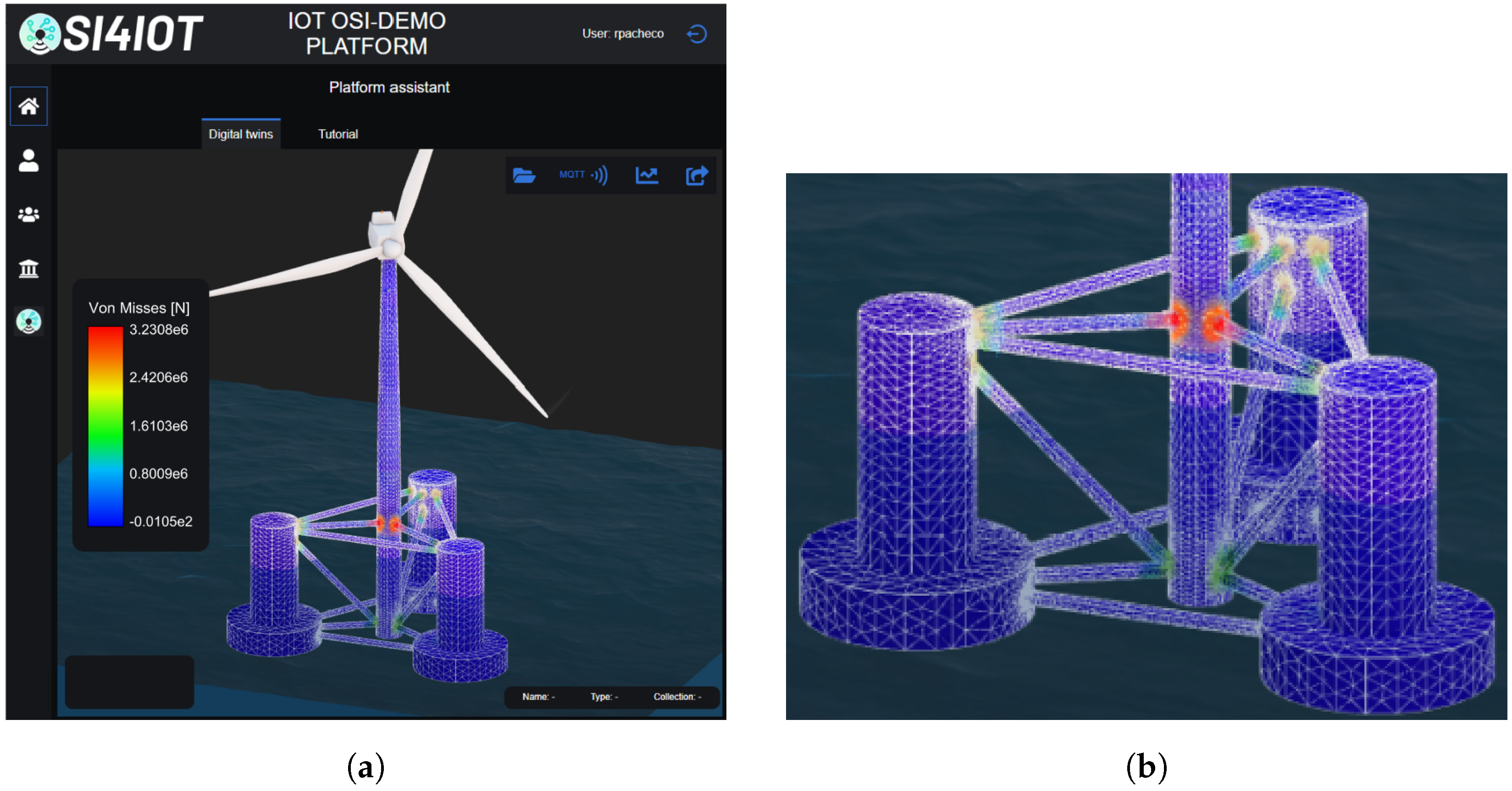
Figure 15 shows the von Mises stress distribution at a representative time step, visualized in three dimensions through the platform’s web interface. High-stress regions appear near structural discontinuities, such as the tower base and brace joints. The stress field is updated in real time, enabling engineers to identify critical areas as environmental conditions evolve.
To evaluate temporal stress fluctuations, the digital twin provides time histories of signed von Mises stress at any structural location. Figure 16 shows an example for a representative element under the reference condition. The alternating tension–compression cycles are clearly captured by the ROM, confirming its ability to reproduce transient load effects at high resolution.
To assess local stress accuracy at the same critical node used for displacement validation, Figure 17 compares the signed von Mises stress histories computed by the ROM and by the full FEM over a 100 s window. The curves overlap across peaks and troughs, indicating that the ROM preserves transient stress reversals and amplitudes with relative deviations below 1% at this location.

5.3. Fatigue

Fatigue damage is assessed by the digital twin based on full stress time series extracted at predefined structural hotspots. A total of 1000 “hot-spot stress read-out points” selected according to the Bureau Veritas guidelines [49], focusing on regions with high stress concentrations or fatigue-sensitive details. For each hotspot, fatigue life is evaluated under the fatigue environmental conditions of 1000 metocean scenarios.
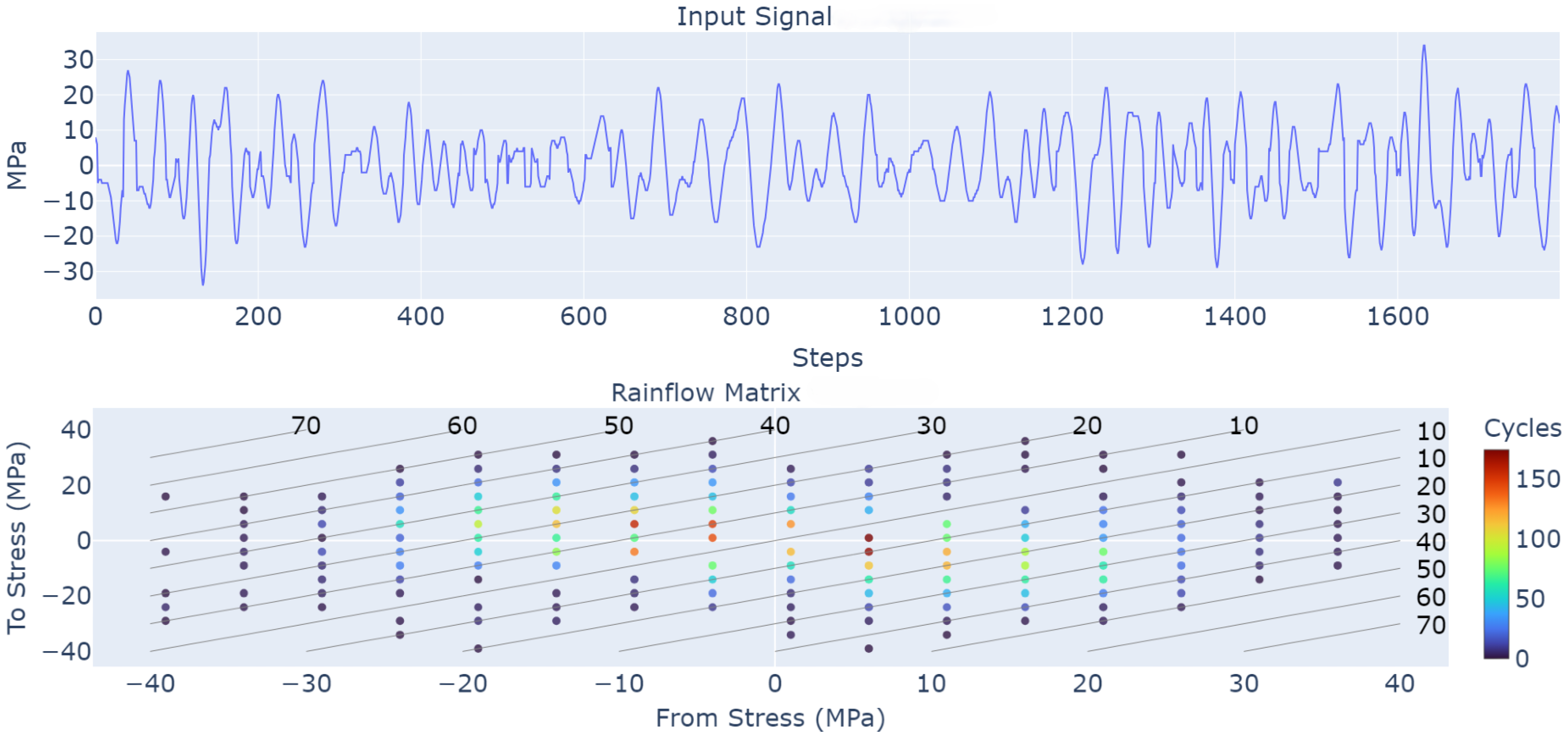
The combination of 1000 hotspots and 1000 environmental scenarios yields one million load cases, each generating a 3 h stress time series. Fatigue analysis follows the recommendations of IEC 61400-3-2 [50], with stress cycles extracted using the four-point rainflow method defined in ASTM E1049-85 [30]. Figure 18 illustrates the raw signal and rainflow matrix for a representative hotspot. The matrix bins stress cycles according to their start and end stress levels, with diagonal bands indicating constant stress ranges. Applying this procedure across all cases enables a full-field fatigue assessment under diverse operating conditions.
This type of analysis supports “what-if” assessments—such as evaluating the impact of an upcoming storm, altered control settings, or extended operation—by estimating fatigue damage at key locations under diverse loading conditions. The fatigue module complements the displacement and stress evaluations, completing the digital twin’s real-time structural monitoring capabilities.

5.4. Real-Time Simulation Performance

A key advantage of the proposed digital twin framework is its ability to execute structural simulations rapidly, supporting real-time monitoring requirements. To assess computational performance, the analysis was benchmarked on a workstation equipped with an AMD Ryzen Threadripper PRO 5995WX CPU and an NVIDIA RTX 4070 Ti GPU. The three primary simulation tasks—displacement, stress, and fatigue evaluation—were executed on both CPU and GPU to compare runtimes across architectures.

5.4.1. Displacement Analysis

The digital twin employs a reduced-order model (ROM) to reconstruct full-field structural displacements efficiently under the reference condition. For a 3 h simulation involving 839 , 256 spatial DOFs and 108,000 time steps—about 9.06 × 10 10 total updates—the ROM completed the task in 14.45 min on a CPU and just 0.69 min on a GPU, corresponding to update rates of 104.5 million and 2.43 billion DOFs per second, respectively. In contrast, the full finite element model (FEM) took over 2235 min to run on the same CPU, with an update rate of only 0.68 million DOFs per second. This represents a speedup of approximately 155× over FEM on CPU, and more than 3200× when using GPU acceleration—reflecting the computational gains achieved through modal superposition and massively parallel integration. These results are summarized in Table 2.

5.4.2. Stress Analysis

Stress evaluation is more computationally intensive than displacement because it updates a far greater number of integration points; the timings reported below correspond to the same reference condition. For each of the 108,000 time steps, stresses were computed at 7,570,008 points, yielding a total of approximately 8.18 × 10 11 stress evaluations. The full simulation required 46.4 min on the CPU and 3.81 min on the GPU. This demonstrates that the digital twin can update the full stress history of the structure in under 4 min, supporting continuous monitoring and fatigue analysis. These results are summarized in Table 3.

5.4.3. Fatigue Analysis

Fatigue analysis was conducted over 1000 critical points and the 1000 fatigue environmental conditions, resulting in 1 million individual stress–time series. Each signal was processed using a cycle-counting algorithm followed by damage accumulation. While the per-signal operations are inherently sequential, GPU parallelism was leveraged across points and scenarios to accelerate computation. The total simulation required 98 min on the CPU and 37 min on the GPU, corresponding to 340 and 901 complete 3 h stress histories processed per second, respectively. This allows the digital twin to generate full-field fatigue forecasts across thousands of conditions in under an hour. In practical applications, scenario subsets can be evaluated in minutes, enabling near-real-time support for maintenance planning. These results are summarized in Table 4. Table 5 reports the average time required per hotspot across 1000 operating scenarios.

6. Conclusions

This study presented a real-time digital twin (DT) framework tailored for the structural health monitoring of floating offshore wind turbines (FOWTs). At its core lies a hydro-elastic reduced-order model (ROM) that captures the turbine’s dominant dynamic behavior and fluid–structure interactions with high fidelity. This physics-based ROM enables the rapid computation of displacements, stresses, and fatigue damage while preserving the accuracy of full finite element models, bridging the long-standing trade-off between physical rigor and real-time performance.
The framework was validated on the OC4-DeepCWind semi-submersible platform, demonstrating that it can reconstruct full-field structural responses with errors consistently below 1%, while achieving runtime reductions in over an order of magnitude. Critically, this includes the capability to perform real-time fatigue assessment across thousands of environmental scenarios, a task traditionally reserved for offline post-processing. These results directly address the initial problem highlighted in the literature: existing DTs are either computationally prohibitive for real-time use or rely on reduced-fidelity, black-box surrogates that lack generalizability and interpretability. By contrast, the presented framework retains physical transparency, generalizes to new load cases, and executes efficiently on standard hardware.
By design, the platform’s structural model is intended to operate within the linear elastic regime, which is adequate for the substructure and tower across the majority of operating conditions. The principal limitations therefore arise from subsystems whose response is intrinsically non-linear—most notably active rotor-blade control, mooring-line dynamics, and other components that experience large displacements or material non-linearities. Ongoing work is focused on embedding specialized non-linear reduced-order models for these subsystems so that the digital twin remains accurate under extreme or highly coupled loading scenarios.
The platform is designed for extensibility: although demonstrated on a steel mono-turbine system, it can be adapted to composite materials and scaled to multi-turbine arrays. This adaptability, combined with integrated real-time visualization and fatigue forecasting, makes it well-suited for deployment in operational settings.
The framework paves the way for scalable deployment in real offshore wind farms, reducing maintenance costs and improving availability of clean energy infrastructure. By closing the loop between high-fidelity physics, efficient computation, and real-time monitoring, this digital twin framework offers a robust and actionable tool for advancing the operational resilience and economic viability of offshore wind energy.

Author Contributions

Conceptualization, A.P.-S., J.G.-E. and D.D.C.; Methodology, A.P.-S., J.G.-E., D.D.C. and B.S.-C.; Software, A.P.-S., J.G.-E., D.D.C. and B.S.-C.; Formal analysis, A.P.-S. and I.B.-P.; Investigation, A.P.-S., J.G.-E. and D.D.C.; Resources, J.G.-E., D.D.C. and B.S.-C.; Writing—original draft, A.P.-S.; Writing—review and editing, J.G.-E. and D.D.C.; Visualization, A.P.-S.; Supervision, J.G.-E. and D.D.C.; Project administration, J.G.-E.; Funding acquisition, J.G.-E. All authors have read and agreed to the published version of the manuscript.

Funding

This research was funded by the Spanish ‘Ministerio de Ciencia e Innovacion’ under the grant agreement MLAMAR (ref. PID2021-126561OB- C31).

Data Availability Statement

The datasets presented in this article are not readily available because they originate from a collaboration with an industrial partner and contain proprietary information protected by contractual confidentiality and non-disclosure agreements. Requests to access the datasets should be directed to Andres Pastor-Sanchez. Access, if granted, will be limited to non-commercial research purposes and subject to a data-sharing agreement and prior approval from the industrial partner.

Acknowledgments

During the preparation of this work, the authors used ChatGPT 4 to improve the language and readability. After using this tool/service, the authors reviewed and edited the content as needed. The authors take full responsibility for the content of this publication.

Conflicts of Interest

The authors declare no conflicts of interest.

References

  1. Taze, I.E.; Hoda, M.A.; Míquelez, I.; Maddaloni, P.; Azam, S.E. A Review of Digital Twinning Applications for Floating Offshore Wind Turbines: Insights, Innovations, and Implementation. Energies 2025, 18, 3369. [Google Scholar] [CrossRef]
  2. León-Medina, J.X.; Tibaduiza, D.A.; Parés, N.; Pozo, F. Digital twin technology in wind turbine components: A review. Intell. Syst. Appl. 2025, 20, 200535. [Google Scholar] [CrossRef]
  3. Augustyn, D.; Ulriksen, M.D.; Sørensen, J.D. Reliability Updating of Offshore Wind Substructures by Use of Digital Twin Information. Energies 2021, 14, 5859. [Google Scholar] [CrossRef]
  4. Jorgensen, J.; Hodkiewicz, M.; Cripps, E.; Hassan, G.M. Requirements for the Application of the Digital Twin Paradigm to Offshore Wind Turbine Structures for Uncertain Fatigue Analysis. Comput. Ind. 2023, 145, 103806. [Google Scholar] [CrossRef]
  5. Yu, Q.; Xu, J. Fatigue reliability assessment of floating offshore wind turbines under correlated wind–wave–current loads. Ocean. Eng. 2024, 313, 119442. [Google Scholar] [CrossRef]
  6. Gaidai, O.; Yakimov, V.; Wang, F.; Zhang, F.; Balakrishna, R. Floating wind turbines structural details fatigue life assessment. Sci. Rep. 2023, 13, 19665. [Google Scholar] [CrossRef]
  7. Moghadam, F.K.; de S. Rebouças, G.F.; Nejad, A.R. Digital Twin Modeling for Predictive Maintenance of Gearboxes in Floating Offshore Wind Turbine Drivetrains. Forsch. Ingenieurwesen 2021, 85, 273–286. [Google Scholar] [CrossRef]
  8. Mehlan, F.C.; Nejad, A.R.; Gao, Z. Digital Twin Based Virtual Sensor for Online Fatigue Damage Monitoring in Offshore Wind Turbine Drivetrains. J. Offshore Mech. Arct. Eng. 2022, 144, 060901. [Google Scholar] [CrossRef]
  9. Walker, J.G.; Coraddu, A.; Collu, M.; Oneto, L. Digital Twins of the Mooring Line Tension for Floating Offshore Wind Turbines to Improve Monitoring, Lifespan, and Safety. J. Ocean Eng. Mar. Energy 2022, 8, 1–16. [Google Scholar] [CrossRef]
  10. Branlard, E.; Jonkman, J.; Brown, C.; Zhang, J. A digital twin solution for floating offshore wind turbines validated using a full-scale prototype. Wind. Energy Sci. 2024, 9, 1–24. [Google Scholar] [CrossRef]
  11. Bull, T.S.; Muff, D.V.; Wagner, P.R.; Zhang, W.H.; Faber, M.H.; Schubert, M.; Riber, H.J. Probabilistic Digital Twin-Informed Risk-Based Inspection Planning for Offshore Wind Turbine Structures. Struct. Health Monit. 2025; in press. [Google Scholar] [CrossRef]
  12. Mousavi, Z.; Varahram, S.; Ettefagh, M.M.; Sadeghi, M.H.; Feng, W.Q.; Bayat, M. A digital twin-based framework for damage detection of a floating wind turbine structure under various loading conditions based on deep learning approach. Ocean. Eng. 2024, 292, 116563. [Google Scholar] [CrossRef]
  13. Simpson, T.; Dervilis, N.; Couturier, P.; Maljaars, N.; Chatzi, E. Reduced order modeling of non-linear monopile dynamics via an AE-LSTM scheme. Front. Energy Res. 2023, 11, 1128201. [Google Scholar] [CrossRef]
  14. Xia, J.; Zou, G. Operation and Maintenance Optimization of Offshore Wind Farms Based on Digital Twin: A Review. Ocean. Eng. 2023, 268, 113322. [Google Scholar] [CrossRef]
  15. Chen, B.Q.; Liu, K.; Yu, T.; Li, R. Enhancing Reliability in Floating Offshore Wind Turbines through Digital Twin Technology: A Comprehensive Review. Energies 2024, 17, 1964. [Google Scholar] [CrossRef]
  16. Kandemir, E.; Hasan, A.; Kvamsdal, T.; Alaliyat, S.A. Predictive Digital Twin for Wind Energy Systems: A Literature Review. Energy Inform. 2024, 7, 68. [Google Scholar] [CrossRef]
  17. Pacheco-Blazquez, R.; Garcia-Espinosa, J.; Di Capua, D.; Pastor Sanchez, A. A Digital Twin for Assessing the Remaining Useful Life of Offshore Wind Turbine Structures. J. Mar. Sci. Eng. 2024, 12, 573. [Google Scholar] [CrossRef]
  18. Garcia-Espinosa, J.; Servan-Camas, B.; Calpe-Linares, M. High Fidelity Hydro-elastic Analysis Using Modal Matrix Reduction. J. Mar. Sci. Eng. 2023, 11, 1168. [Google Scholar] [CrossRef]
  19. Servan-Camas, B.; Berdugo-Parada, I.; Garcia-Espinosa, J.; Pastor-Sanchez, A. Modal Matrix Reduction for Fully Coupled Integrated Load Analysis of Floating Structures. Mar. Struct. 2025, 103, 103845. [Google Scholar] [CrossRef]
  20. Servan-Camas, B.; Gutierrez-Romero, J.E.; Garcia-Espinosa, J. A Time-Domain Second-Order FEM Model for the Wave Diffraction-Radiation Problem. Validation with a Semisubmersible Platform. Mar. Struct. 2018, 58, 278–300. [Google Scholar] [CrossRef]
  21. International Renewable Energy Agency. Future of Wind: Deployment, Investment, Technology, Grid Integration and Socio-Economic Aspects; Technical Report; IRENA: Abu Dhabi, United Arab Emirates, 2019. [Google Scholar]
  22. Global Offshore Wind Alliance. Offshore Wind: From 83 GW Today to 2,000 GW by 2050; IRENA and GOWA Initiative; IRENA: Abu Dhabi, United Arab Emirates, 2025. [Google Scholar]
  23. Center for Sustainable Systems, University of Michigan. Wind Energy Factsheet; Pub. No. CSS07-09; University of Michigan: Ann Arbor, MI, USA, 2024. [Google Scholar]
  24. Averroes.ai. Wind Turbine Maintenance & Inspection: Offshore, Cost, Blades; Averroes.ai: San Mateo, CA, USA, 2024. [Google Scholar]
  25. SANY Heavy Energy. SANY Heavy Energy Realizes High-Precision Wind Turbine Simulation with Siemens Simcenter 3D; Case Study: 10% LCOE Reduction Through Digital Twin Implementation; SANY Heavy Energy: Changsha, China, 2023. [Google Scholar]
  26. Dimitrov, N.; Jacquet, C.; Marelli, S. Innovative models slash offshore wind energy costs by 9%. TechXplore 2024. [Google Scholar]
  27. Servan-Camas, B.; Di-Capua, D.; Garcia-Espinosa, J.; Sa-Lopez, D. Fully 3D ship hydro-elasticity: Monolithic versus partitioned strategies for tight coupling. Mar. Struct. 2021, 80, 103098. [Google Scholar] [CrossRef]
  28. Bathe, K.J. Finite Element Procedures; K.J. Bathe: Watertown, MA, USA, 2016. [Google Scholar]
  29. Branlard, E.; Jonkman, J.; Dana, S.; Doubrawa, P. A digital twin based on OpenFAST linearizations for real-time load and fatigue estimation of land-based turbines. J. Phys. Conf. Ser. 2020, 1618, 022030. [Google Scholar] [CrossRef]
  30. ASTM E1049-85(2017); Standard Practices for Cycle Counting in Fatigue Analysis. ASTM: West Conshohocken, PA, USA, 2017. [CrossRef]
  31. Software, S.D.I. Calculating Damage with Miner’s Rule. 2023. Available online: https://community.sw.siemens.com/s/article/calculating-damage-with-miner-s-rule (accessed on 10 September 2025).
  32. Ltd, O. Fatigue Analysis: S–N and T–N Curves. 2025. Available online: https://www.orcina.com/webhelp/OrcaFlex/Content/html/Fatigueanalysis,S-NandT-Ncurves.htm (accessed on 10 September 2025).
  33. Siemens. Rainflow Counting Method. 2019. Available online: https://community.sw.siemens.com/s/article/rainflow-counting (accessed on 10 September 2025).
  34. React Documentation Team. React—The JavaScript Library for Building User Interfaces. 2025. Available online: https://legacy.reactjs.org/ (accessed on 10 September 2025).
  35. Node-RED Team. Node-RED. 2025. Available online: https://nodered.org/ (accessed on 10 September 2025).
  36. Eclipse Mosquitto Project. Eclipse Mosquitto. 2025. Available online: https://projects.eclipse.org/projects/iot.mosquitto (accessed on 10 September 2025).
  37. Timescale, Inc. TigerData—The Fastest Postgres Cloud for Real-Time Analytics, Time Series, AI & Vector Workloads; d/b/a TigerData; Timescale, Inc.: New York, NY, USA, 2025. [Google Scholar]
  38. Grafana Labs. Grafana—Dashboard Anything. Observe Everything; Grafana Labs: New York, NY, USA, 2025. [Google Scholar]
  39. PyTorch Foundation. PyTorch—An Open Source Machine Learning Framework; PyTorch Foundation: San Francisco, CA, USA, 2025. [Google Scholar]
  40. Compass Ingeniería y Sistemas, S.A. Structural Analysis—Tdyn RamSeries; Compass Ingeniería y Sistemas, S.A.: Barcelona, Spain, 2025. [Google Scholar]
  41. Blender Foundation. Blender—Free and Open Source 3D Creation Software; Blender Foundation: Amsterdam, The Netherlands, 2025. [Google Scholar]
  42. OpenWeather Ltd. OpenWeatherMap—Global weather data & APIs; OpenWeather Ltd.: London, UK, 2025. [Google Scholar]
  43. Puertos del Estado. Portus—Marine and Ocean-Meteorological Data for Spain’s Port System; Puertos del Estado: Madrid, Spain, 2025. [Google Scholar]
  44. Copernicus Programme/European Commission. Copernicus—The European Union’s Earth Observation Programme. 2025. Available online: https://www.copernicus.eu/sites/default/files/Brochure_Copernicus_2019%20updated_0.pdf (accessed on 10 September 2025).
  45. EnerOcean, S.L. W2Power—The Future of Floating. Now. 2025. Available online: https://enerocean.com/w2power/ (accessed on 10 September 2025).
  46. FIBREGY Consortium. FIBREGY—Composites for a Sustainable Environment. 2025. Available online: https://fibregy.eu/ (accessed on 10 September 2025).
  47. OPeNDAP, Inc. OPeNDAP—Open-source Project for a Network Data Access Protocol; OPeNDAP, Inc.: Butte, MT, USA, 2025. [Google Scholar]
  48. DeepCWind Company. DeepCWind Company—Accelerating the Future of Floating Offshore Wind; DeepCWind Company: Orono, ME, USA, 2025. [Google Scholar]
  49. Bureau Veritas Marine & Offshore. Guidelines for Fatigue Assessment of Ships and Offshore Units (Rule Note NI 611); Bureau Veritas Marine & Offshore: Courbevoie, France, 2020. [Google Scholar]
  50. IEC 61400-3-2:2025; Wind Turbines—Part 3-2: Design Requirements for Floating Offshore Wind Turbines. International Electrotechnical Commission: London, UK, 2025.
Figure 1. Typical modal energy distribution and the cumulative energy captured [18].
Jmse 13 01953 g001
Figure 2. Reconstruction of displacement through linear combination of modal base and modal amplitudes.
Jmse 13 01953 g002
Figure 3. Application of the 4-point Rainflow counting algorithm to a discretized stress history [33]: (a) 4-point Rainflow window on a discretized stress history; (b) cycle closures identified by the 4-point rule.
Jmse 13 01953 g003
Figure 4. Mind map of the digital twin pipeline: data ingestion, storage, compute, and visualization.
Jmse 13 01953 g004
Figure 5. Containerized architecture of OSI4IOT: isolated services for frontend (React), automation (Node-RED), and sensor communication (Mosquitto).
Jmse 13 01953 g005
Figure 6. Real-time Grafana dashboard displaying structural and environmental signals, including strain, displacement, and wind data.
Jmse 13 01953 g006
Figure 7. Data integration workflow. Mesh data are imported into Blender; simulation results are sent directly to OSI4IOT. Blender exports an enriched glTF model for interactive visualization.
Jmse 13 01953 g007
Figure 8. Example of a virtual sensor: external wind forecast integrated into the DT and processed identically to physical measurements.
Jmse 13 01953 g008
Figure 9. Wind sensor installed on the W2Power platform [45], capturing local wind speed and direction in real time as part of the FIBREGY European project [46].
Jmse 13 01953 g009
Figure 10. Finite–element mesh of the OC4 used in the Digital Twin analysis. (a) Global finite–element mesh. (b) Detail view of mesh refinement at a brace–column joint.
Jmse 13 01953 g010
Figure 11. Representative deformation shapes of four vibration modes retained in the ROM. Mode 7 corresponds to the first elastic mode; the six lower-frequency modes are rigid–body motions.
Jmse 13 01953 g011
Figure 12. Digital twin visualization of the wind turbine displacement at a representative time step.
Jmse 13 01953 g012
Figure 13. Comparison of FEM (left) and ROM (right) displacement fields at a representative time step. The ROM closely matches the FEM result with significantly reduced computational cost.
Jmse 13 01953 g013
Figure 14. Validation at a critical node: (a) node location; (b) displacement history (ROM vs FEM) over 100 s.
Jmse 13 01953 g014
Figure 15. von Mises stress field computed with the ROM for the OC4-DeepCWind platform at a representative time step. (a) ROM von Mises stress field over the entire structure. (b) Detail view of the ROM von Mises stress field near the tower base and brace joints.
Jmse 13 01953 g015
Figure 16. Signed von Mises stress σ v m ± under combined wind and wave loading. (Left) 3D view showing the element of interest. (Right) time history of σ v m ± at the three Gauss points, clearly illustrating alternating tensile (positive) and compressive (negative) cycles.
Jmse 13 01953 g016
Figure 17. Stress validation at a critical node: (a) node location; (b) signed von Mises stress time-history comparison over 100 s.
Jmse 13 01953 g017
Figure 18. Fatigue analysis at a representative hotspot. (Top) Stress time series over a 3 h simulation. (Bottom) Rainflow matrix showing the number of counted cycles for each pair of reversal points, with the horizontal and vertical axes corresponding to the start and end stress of each cycle. Diagonal lines indicate constant stress ranges, and color represents the number of occurrences.
Jmse 13 01953 g018
Table 1. Key characteristics of the OC4-DeepCWind platform.
CharacteristicValueUnit
Wind turbine rating5MW
Platform mass (incl. ballast)14,077t
Center of mass below SWL11.06m
Center of buoyancy below SWL13.15m
Draft20m
Main column diameter6.25m
Offset column upper diameter12m
Offset column base diameter24m
Column spacing (triangle side)50m
Mooring lines3
Mooring line length835.5m
Anchor radius837.6m
Fairlead radius40.87m
Roll inertia 1.12 × 10 10 kg·m2
Pitch inertia 1.11 × 10 10 kg·m2
Yaw inertia 1.13 × 10 10 kg·m2
Hub height90m
Water depth200m
Mooring systemCatenary
Table 2. Displacement computation benchmark for a 3 h simulation (839,256 DOFs, 108,000 time steps). The table compares the total runtime and update rate of the Reduced-Order Model (ROM) on CPU and GPU against the full finite element method (FEM) on CPU.
ROMFEM
CPUGPUCPU
Simulation Time14.45 min0.69 min2 235 min
Update Rate104.5 million DOFs/s2.43 billion DOFs/s0.68 million DOFs/s
Table 3. Benchmark results for the digital twin stress computation over a 3 h simulation involving 7,570,008 evaluation points and 108,000 time steps. The table reports total runtimes and update rates for CPU and GPU executions.
CPUGPU
Simulation Time46.4 min3.81 min
Update Rate293.5 million points/s3.57 billion points/s
Table 4. Benchmark results for fatigue analysis across 1000 critical points and 1000 operating scenarios (1 million time series). Reported values include total simulation time and average processing rate for CPU and GPU implementations.
CPUGPU
Simulation Time98 min37 min
Processing Rate340.1 stress histories/s901.4 stress histories/s
Table 5. Average time required to compute fatigue damage for one structural hotspot across 1000 operating scenarios.
CPUGPU
Time per Hotspot (1000 Scenarios)2.94 s1.10 s
Disclaimer/Publisher’s Note: The statements, opinions and data contained in all publications are solely those of the individual author(s) and contributor(s) and not of MDPI and/or the editor(s). MDPI and/or the editor(s) disclaim responsibility for any injury to people or property resulting from any ideas, methods, instructions or products referred to in the content.