Abstract
Currently, maritime navigation safety risks—particularly those related to ship navigation—are primarily assessed through traditional rule-based methods and expert experience. However, such approaches often suffer from limited accuracy and lack real-time responsiveness. As maritime environments and operational conditions become increasingly complex, traditional techniques struggle to cope with the diversity and uncertainty of navigation scenarios. Therefore, there is an urgent need for a more intelligent and precise risk prediction method. This study proposes a ship risk prediction framework that integrates a deep learning model based on Long Short-Term Memory (LSTM) networks with Bayesian risk evaluation. The model first leverages deep neural networks to process time-series trajectory data, enabling accurate prediction of a vessel’s future positions and navigational status. Then, Bayesian inference is applied to quantitatively assess potential risks of collision and grounding by incorporating vessel motion data, environmental conditions, surrounding obstacles, and water depth information. The proposed framework combines the advantages of deep learning and Bayesian reasoning to improve the accuracy and timeliness of risk prediction. By providing real-time warnings and decision-making support, this model offers a novel solution for maritime safety management. Accurate risk forecasts enable ship crews to take precautionary measures in advance, effectively reducing the occurrence of maritime accidents.
1. Introduction
Maritime transportation serves as a vital component of global trade networks. While burgeoning trade volumes present development opportunities for shipping industry, they also introduce challenges associated with vessel gigantism and route congestion. Contemporary maritime systems face growing pressures from intensifying sea lane utilization and port operations, leading to increased maritime accident risks [1].
Maritime risk prediction confronts inherent complexity due to multifaceted influencing factors including environmental conditions and vessel behaviors. Reliable real-time prediction systems are crucial for supporting operational decisions to mitigate potential losses. Consequently, developing accurate vessel trajectory and collision risk prediction algorithms has become essential for maritime safety.
In recent years, scholars have suggested several ship trajectory prediction models. Jaskólski [2] used discrete Kalman filter to estimate missing ship trajectory sequences based on AIS data. Fossen and Fossen [3] used extended Kalman filter (EKF) to process real-time AIS data, predict the future motion of ships and analyze evasion strategies to avoid collision. Zhang [4] proposed a trajectory prediction algorithm for Hidden Markov Models based wavelet transform (HMM-WA). Specifically, the ship trajectory sequence is transformed into a column vector by wavelet transform and single reconstruction. Then the vector is used as the input of HMM, and the future position of the ship is estimated by Markov chain. These methods have been highly successful for navigation-grade state estimation and short-horizon prediction when the motion/process model is appropriately specified. In this study, the intended limitation is not that these methods can “only” predict the next position, but that in common AIS-only settings with simple, low-order kinematic or linear-Gaussian assumptions and without explicit maneuver/intent or interaction modeling, single-model KF/EKF/HMM tend to yield smooth extrapolations that degrade over longer horizons and under complex, multi-modal behaviors (e.g., abrupt maneuvers, interactions with other vessels, route/traffic rules, and environmental/terrain constraints).
These limitations can be mitigated by incorporating higher-fidelity dynamics, multi-model approaches (e.g., Interacting Multiple Model (IMM)), nonlinear/unscented or particle filters, and context/constraint information, but such extensions go beyond the baseline configurations compared in this section.
Operational shipboard decision support systems must pull heterogeneous, location-dependent information in real time—including AIS traffic, Electronic Navigational Charts (ENC) with bathymetry and hazards, fairway geometry, and short-term environmental context such as wind, waves, and currents—under strict latency, coverage, and reliability constraints. However, many trajectory-prediction and risk-assessment studies implicitly assume oracle access to perfect, static maps or offline annotations, creating a sim-to-real gap when methods are moved onboard. In constrained waterways, this gap manifests as depth and obstacle priors that are incomplete or not aligned to the vessel’s geodetic frame, dynamic context (temporary obstructions, traffic density, tidal windows) that is time-varying, and query patterns that must be localized to the predicted path rather than global. To bridge this, we introduce a database module that emulates shipborne data acquisition: given a predicted motion sequence, it serves trajectory-conditioned queries (e.g., nearest obstacle, depth-along-track, encounter configuration, traffic statistics) at runtime with an update cadence compatible with onboard use. This design grounds learning-based predictors and Bayesian risk reasoning in the same information surfaces available to actual vessels, enabling auditable, chart-aware inference.
Ship navigation risk assessment faces a three-way tension among data uncertainty, subjectivity/timeliness, and compute/latency. Grey System Theory is attractive under missing or sparse navigation data and can extrapolate trends for decision support, yet it typically suffers from lower precision, rapid decay/growth behaviors, and limited timeliness when risks evolve quickly [5,6,7,8]. Traditional expert-driven models work with limited data but are sensitive to subjective judgments, lack cross-expert consistency, and struggle to deliver real-time perception, making them ill-suited for online prediction [7,8]. At the other end, deep-learning approaches reduce subjectivity and fuse multimodal inputs with strong fitting capacity, but they demand substantial data and high-performance computing, and can exhibit training/gradient issues on long sequences, which hampers low-latency online deployment in dynamic waterways [9,10]. While Informer-style architectures alleviate part of the latency/throughput bottleneck via efficient self-attention—enabling faster parallel processing for online forecasting—their assessments remain largely black-box and do not natively quantify or propagate epistemic/aleatoric uncertainty or encode causal structure among risk factors [11]. In contrast, Bayesian networks have been successfully used to identify navigation risk factors in data-scarce regions (e.g., Arctic waters) and offer interpretable, uncertainty-aware reasoning that can ingest heterogeneous, partially missing evidence and update beliefs online [12]. These limitations collectively motivate our Bayesian risk prediction module, which complements the trajectory predictor by producing posterior risk estimates with traceable assumptions for decision support under real-world data imperfections.
To address the above limitations, we develop an End-to-End, three-tier framework that couples a CNN-BiLSTM- Multi-Head Self-Attention (MHSA) trajectory predictor with an ENC-aware spatial database and a Bayesian dynamic risk network, and closes the loop with an onboard-style decision layer. The system runs with sliding-window updates, performs path-conditioned chart queries around the predicted motion, and outputs interpretable posterior risks and real-time guidance under strict latency constraints. The main contributions are as follows:
- Hybrid Spatio-Temporal Trajectory Prediction: This innovation combines Convolutional Neural Networks (CNN), Bidirectional Long Short-Term Memory (BiLSTM) networks, and Multi-Head Attention mechanisms to overcome the shortcomings of single-model approaches in ship trajectory forecasting. Specifically:
- (1)
- CNN layers extract localized patterns from short-term motion data (e.g., speed fluctuations or heading adjustments).
- (2)
- Multi-Head Attention dynamically weights key historical time steps, focusing on critical navigation segments.
- (3)
- BiLSTM processes sequential data bidirectionally, capturing long-range dependencies for robust predictions.
- Electronic Navigational Chart (ENC)-Aware Spatial Database: We developed a dynamic spatial query system that bridges the “sim-to-real gap” by providing real-time environmental context based on predicted trajectories. Key features include:
- (1)
- Trajectory-conditioned queries that retrieve obstacle distributions and bathymetric data (e.g., water depth) along a vessel’s path.
- (2)
- Spatial indexing (e.g., R-trees) for efficient obstacle and depth retrieval within a local radius, reducing reliance on static maps.
- (3)
- Database schema with hierarchical tables for navigational aids, bathymetric areas, and dynamic elements, ensuring consistency with shipboard data surfaces.
- This enables real-time scene awareness, supporting accurate risk evaluation in dynamic waterways.
- Bayesian Risk Prediction with Interpretable Posteriors: A Bayesian network framework quantifies collision and grounding risks transparently, Specifically:
- (1)
- Evidence integration: Combines vessel motion data (position, SOG, COG), environmental factors (obstacle distance, water depth), and external conditions (e.g., weather) into a probabilistic model.
- (2)
- Dynamic inference: Uses Variable Elimination to compute posterior probabilities in real time.
- Closed-Loop Decision Support System: This innovation closes the feedback loop from prediction to action, enabling minute-level risk warnings and proactive navigation control:
- (1)
- Integrated workflow: Links trajectory prediction, environment querying, Bayesian inference, and action suggestions in a seamless cycle with <5 s latency.
- (2)
- Actionable outputs: Maps risk probabilities to International Regulations for Preventing Collisions at Sea (COLREGs)-compliant maneuvers, such as course adjustments (θnew = θcurrent + θoptimal) or speed reductions
- (3)
- Real-time performance: Operates via sliding-window updates, maintaining system stability and responsiveness even with data anomalies.
This transforms passive monitoring into active risk mitigation, supporting safer maritime operations.
This study used the Operating System (windows11 23h2); Python (3.9); MySQL Server (8.0); MySQL client/driver—PyMySQL (1.1.2); TensorFlow/Keras (2.16.1); scikit-learn (1.6.0); NumPy (1.23.5); pandas (2.2.3); Matplotlib (3.9.1); Seaborn (0.13.2); NetworkX (3.2.1); pgmpy (0.1.26); graphviz (Python package) (0.20.3) and PyGraphviz (1.11); pyproj (3.7.1).
2. Related Work
2.1. Data-Driven Deep Learning for Vessel Trajectory Prediction
Data-driven approaches analyze large-scale datasets to capture motion patterns and spatial-temporal characteristics. Predicting future trajectories remains challenging due to inherent uncertainties in vessel behaviors and complex inter-ship correlations. Existing methods often overlook the persistence and cross-domain nature of vessel interactions [13].
Miaomiao Wang proposed a Spatio-Temporal Cross hybrid Network (STCNet) framework, comprising spatio-temporal interaction awareness and multi-modal trajectory prediction modules, which performs adaptive fusion of temporal, spatial, and cross-domain feature [14]. Huanhuan Li et al. developed a cascaded network model integrating Bidirectional LSTM (BiLSTM) and Bidirectional GRU (BiGRU) into a three-layer information enhancement architecture [15]. Wenjun Zhang et al. introduced the DGCN-Transformer model that incorporates collision risk modeling into the prediction framework [16].
Zhiheng Liu proposed an ensemble model containing two sub-models, where the S-TGP model combines Temporal Convolutional Networks (TCN) with Gated Recurrent Units (GRU) to leverage their respective advantages [17]. Huanhuan Li further proposed a new bidirectional information fusion-driven model addressing limitations of classical methods, developing a cascaded network through sequential combination of BiLSTM and BiGRU [18]. Xi Zeng developed the ST-GRUA model based on GRU and self-attention mechanisms for multi-vessel encounter prediction using AIS data [19].
Jinqiang Bi et al. constructed spatio-temporal matrices incorporating navigational geography factors, establishing a CNNGRU-MHA hybrid model with multi-head attention [20]. Hee-Jin Lee employed CNN-LSTM models for trajectory prediction and collision assessment across vessels with different maneuverability characteristics [21].
Xiliang Zhang et al. proposed the G-STGAN method featuring: (1) Ship Spatial Gate Encoder (SSGE) combining Graph Convolutional Network (GCN) and Transformer; (2) Ship Temporal Gate Encoder (STGE) using gated Transformer and temporal convolution [22]. Siwen Wang et al. developed the STPGL model integrating LSTM with graph attention networks (GAT) in an encoder–decoder architecture [23]. Daiyong Zhang established ultra-short-term prediction models based on ship response characteristics, proposing velocity distribution extraction and online error correction algorithms [24].
The trajectory-prediction literature has evolved from sequential encoders to hybrid CNN/attention/graph designs, increasingly emphasizing interaction awareness and geographic grounding. However, there remains a gap between high-capacity models and shipboard constraints (latency, explainability, standards compliance). The database- and chart-aware integration adopted later in this paper directly targets that gap by aligning inputs and outputs with operational Electronic Chart Display and Information System (ECDIS)/ENC contexts.
2.2. Navigation Risk Prediction and Assessment
Current maritime risk prediction integrates traditional statistical analysis with modern intelligent techniques. Traditional approaches establish probabilistic models (e.g., collision/grounding probability models) based on historical accident data, incorporating expert systems and fuzzy logic to quantify risk weights of environmental, operational, and vessel status factors. Modern methods employ machine learning (e.g., neural networks, random forests) and multi-source data fusion (AIS, meteorological, hydrological, and GIS data) for dynamic risk assessment through feature extraction and pattern recognition. Research trends emphasize real-time data-driven hybrid models combining Bayesian networks and deep reinforcement learning, though challenges persist in model interpretability, data quality dependency, and multi-factor coupling mechanisms.
Hanwen Fan et al. developed a Dynamic Bayesian network (DBN) framework addressing imbalanced accident reports through synthetic minority oversampling and edited nearest neighbor techniques [25]. In subsequent work, they proposed an architecture integrating outlier and missing data processing to construct comprehensive databases for Bayesian network construction [26]. Ryan Wen Liu et al. introduced a collision risk analysis framework incorporating quaternion ship domains (QSD) into vessel conflict ranking operators (VCRO) [27].
Wenyang Wang et al. established a Bayesian network model analyzing 549 maritime accidents from 2016 to 2023 in the RCEP region, identifying key factors including accident type, vessel flag, and environmental conditions [28]. Haiyang Jiang et al. constructed Bayesian networks using 55,469 accident records (2002–2022), modeling risk influencing factors (RIF) interdependencies via Tree-Augmented Naive (TAN) networks [29]. Qian Qiao proposed a Risk-Based Ship Complex Network (RBSCN) model with comprehensive node importance algorithms combining degree centrality and betweenness metrics [30].
Dawei Gao et al. developed a predictable Transformer network with clustering analysis for regional collision risk assessment [31]. Wenyang Wang’s team replicated their Bayesian methodology with expanded GISIS datasets [28]. Wenjie Li et al. created an Arctic risk assessment tool calculating event probabilities by incident type and sub-region [14]. Ryan Wen Liu enhanced their framework with kernel density estimation (KDE) for collision risk visualization [27].
Sheng Xu proposed a hybrid causal logic model estimating icebreaker collision probabilities considering human factors [32]. Chenyan Lin et al. designed an encoder–decoder LSTM model with CNN spatial feature extraction for regional collision risk prediction [33]. Peiru Chen et al. established evidence-based fuzzy Bayesian networks using expert-evaluated accident causation networks [34]. Ziaul Haque Munim et al. implemented automated machine learning for operational safety decisions using 40-year Norwegian accident data [35].
Regarding nautical chart integration, Xin Yang et al. developed an Electronic Navigational Chart (ENC)-based grounding risk index (GRI) using fuzzy theory [36]. Cailei Liang designed ENC-based route planning via Delaunay triangulation (DT) of bathymetric data [37].
For multi-task fusion, Tao Liu et al. proposed a deep learning model simultaneously predicting trajectories and collision risks through virtual channel constraints [38]. Our work extends this by integrating automated chart queries and dual risk prediction (collision/grounding). Renan Guedes Maidana demonstrated risk-aware trajectory planning for autonomous vessels [39]. TRYM TENGESDAL implemented GPU-accelerated model predictive control with obstacle avoidance [40].
Belief-space alignment to our pipeline. Following Kochenderfer’s decision-making framework, we treat ship navigation as partially observable sequential control: noisy AIS/ENC observations update a belief over encounter states, and actions (speed/heading changes) are selected to minimize expected cost subject to safety constraints [41,42,43]. In our system, the trajectory predictor provides a tractable surrogate for the state-transition model, while the Bayesian risk head acts as a compact belief updater over collision/grounding variables with soft evidence; the decision mapper then converts posteriors into COLREGs-consistent advisories under thresholds/hysteresis tuned for real-time use (Section 3.3 and Section 3.4). Compared with a full POMDP online planner (e.g., RAO*/ConstrainedZero-style chance-constrained planning) [44], our design trades global optimality for deterministic latency and interpretability, which is critical for on-board deployment and auditability by watch officers and regulators.
Across these streams, internationally recognized principles of multi-agent collision avoidance (e.g., Velocity Obstacles; Optimal Reciprocal Collision Avoidance (ORCA)) and decision-making under uncertainty (e.g., POMDP formulations and reinforcement learning textbooks) provide a unifying lens for modeling risk, quantifying uncertainty, and mapping posteriors to actions. In parallel, regulatory and charting standards (COLREGs; International Hydrographic Organization (IHO) S-57/S-101 [45,46,47]; International Electrotechnical Commission (IEC) 61174) [48] define the compliance and data-integrity requirements that any practical system must satisfy. Our study operationalizes these foundations by: grounding predictions in ENC-aware queries; using a Bayesian network to produce interpretable, uncertainty-aware posteriors, and translating those posteriors into COLREG-aligned guidance under real-time constraints—thereby connecting international theory and standards to deployable maritime safety functions. For a list of relevant references, see Table 1.

Table 1.
Summary table of Literature review.
2.3. Decision-Making Under Uncertainty and POMDPs
A complementary line of work views navigation and collision avoidance as sequential decision-making under uncertainty, formalized by partially observable Markov decision processes (POMDPs). Kochenderfer’s textbooks synthesize the mathematical foundations and scalable algorithms for belief-space planning, including filtering, value iteration/approximation, Monte-Carlo tree search, and risk-aware decision criteria, with applications ranging from airborne collision avoidance to medical decision support [41,42,43]. The ACAS X program in particular demonstrates how dynamic programming and large-scale policy optimization can yield real-time, standard-compliant advisories under strict safety and latency constraints [49].
Compare & contrast. POMDP formulations provide an optimality-theoretic lens (expected utility under partial observability) and naturally capture sensor noise, intent uncertainty, and multi-modal futures—aspects that pure sequence predictors or static classifiers often sidestep. However, general POMDP solvers can be computationally intensive (curse of dimensionality/history) for embedded, high-rate maritime settings, and they require careful state/observation design plus safety constraints (e.g., chance-constraints) to be deployable [49]. Our approach adopts the belief-space perspective to structure information flow, but instantiates a lightweight surrogate: a CNN–MHSA–BiLSTM predictor supplies state-transition surrogates, and a Bayesian network performs interpretable, low-latency belief updates over critical risk factors; decisions are then mapped to COLREGs-consistent advisories (Section 3.3 and Section 3.4). This yields many operational benefits of belief-space reasoning (uncertainty-aware, auditable, sequential) while keeping compute predictable for shipboard hardware.
3. Model Structure: End-to-End Ship Navigation Risk Prediction Model
3.1. Overall Framework Overview
The overall architecture is illustrated in Figure 1. The interfaces of each module are summarized below; implementation details follow in Section 3.2 and Section 3.3.
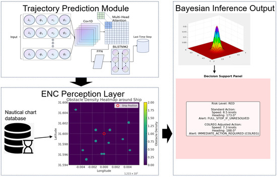
Figure 1.
Three-Layer Architecture of the End-to-End Risk Prediction System.
- (1)
- Trajectory predictor—Input: AIS window of length T with {x, y, speed over ground (SOG), course over ground (COG)}; Output: next-step {x, y, SOG, COG} (+ optional uncertainty).
- (2)
- ENC perception—Input: predicted path polyline; Output: distances to static obstacles, local bathymetry, fairway width, and proximity features.
- (3)
- Bayesian risk head—Input: predictor outputs + ENC features (+ optional weather); Output: posterior P(collision)/P(grounding) and three-tier alert {Green, Yellow, Red}.
3.2. Data Processing
3.2.1. AIS Data Processing
We standardize AIS trajectories through a four-stage pipeline—quality control, anomaly screening, uniform resampling, and navigation-mode labeling—to supply consistent, low-noise sequences for downstream models. The pipeline retains only decisions that materially change the sequence used by the predictor (Figure 2).
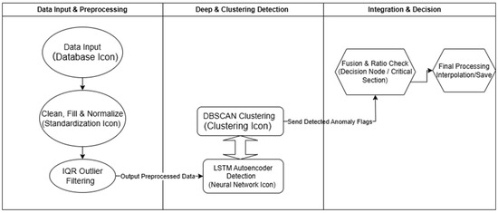
Figure 2.
AIS Preprocessing Pipeline.
Processing pipeline:
- (1)
- Quality control. Remove records with invalid MMSI/coordinates/time order; deduplicate near-identical timestamps; drop speeds outside physically feasible bounds.
- (2)
- Anomaly screening. Detect spikes in SOG/COG and spatial outliers using simple thresholds plus a density-based check; flagged points are treated as missing and will not inform the model.
- (3)
- Uniform resampling. Rebuild each trajectory on a fixed interval (Δt), using distance-aware interpolation to preserve local kinematics; sequences are truncated/padded to a fixed window length T.
- (4)
- Navigation-mode labeling. Assign coarse modes (e.g., cruising, maneuvering, anchoring) from speed/turn-rate rules to provide optional context features.
Key settings. We use a fixed window length T and a fixed resampling interval Δt. Speeds are constrained to a practical operating range, and the turn-rate is bounded by |ΔCOG/Δt|. The outlier density check uses neighborhood radius ε and minPts selected on validation tracks and kept fixed across experiments.
The cleaned, uniformly sampled sequences feed the trajectory predictor in Section 3.3, with no additional per-dataset tuning beyond these fixed settings.
Figure 2 AIS preprocessing pipeline:
- (1)
- quality control;
- (2)
- anomaly screening;
- (3)
- uniform resampling;
- (4)
- navigation-mode labeling.
An example of the preprocessing effect and the resulting route structure is provided in Figure 3 and Figure 4.
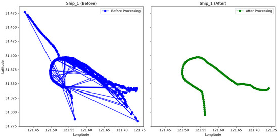
Figure 3.
Results of Hybrid Anomaly Detection and Trajectory Interpolation.
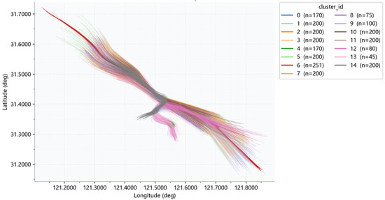
Figure 4.
Trajectory Clustering and Navigation Mode Classification.
3.2.2. Nautical Chart Data Processing and Database Construction
We maintain a lightweight, ENC-aware spatial store to supply the Bayesian head with reliable environmental evidence at shipboard speed. Raw nautical information (e.g., S-57 aids to navigation, fairways/traffic lanes, and bathymetry) is normalized to a common coordinate reference system (CRS) and time base, then compacted into a minimal schema optimized for short-radius queries around the predicted vessel position. Online queries return distance/relative bearing to obstacles and excess water depth along the forecast track, forming standardized inputs for posterior risk estimation.
We materialize four stable entities—areas (bathymetry & regions), line_features (fairways/isobaths), symbols/light_symbols (aids to navigation), and tide_data—plus a small set of spatial functions. Queries operate within a local corridor around the predicted path and output (distance, bearing, class) for obstacles and excess depth along waypoints. Implementation follows common Geographic Information System (GIS) practice and is tuned for sub-second retrieval on onboard hardware. Table 2 summarizes the four runtime entities and the essential fields used by the ENC-aware store.
Table 2.
Entities kept in the ENC-aware store and the essential fields used at runtime.
Practical notes:
- (1)
- Sources are harmonized to a single CRS and Coordinated Universal Time (UTC) timestamps to avoid runtime transforms.
- (2)
- Distance/bearing are computed against the forecasted waypoints, not just the current fix, to align with lead-time evaluation.
- (3)
- Geometry fields are indexed and basic integrity checks (e.g., angle ranges, symbol sizes) are enforced to keep queries robust under noisy inputs.
The format of this database is shown in Figure 5.
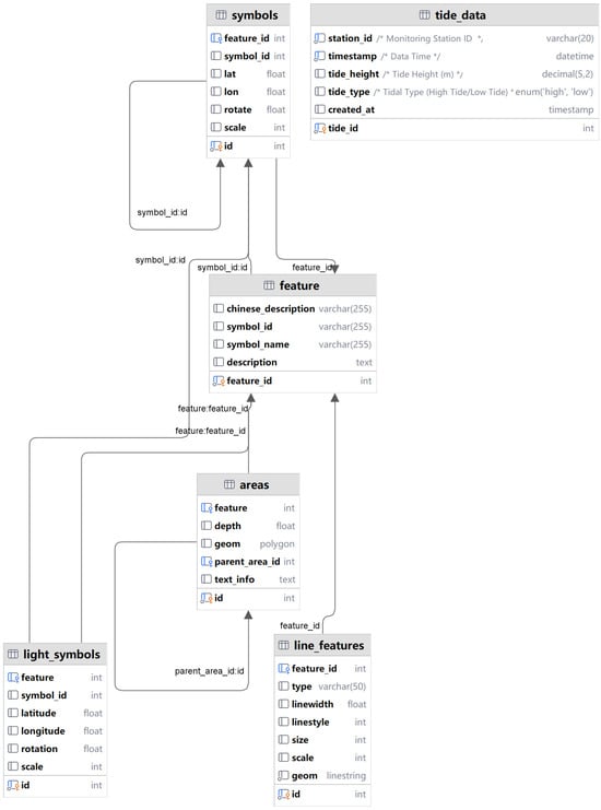
Figure 5.
Spatial Database Schema for Environmental Awareness.
3.3. Trajectory–Risk Collaborative Prediction Model
To address the limitations of single-task models, this study proposes a multi-task collaborative learning framework that integrates ship behavior modeling and environmental risk inference. The model jointly predicts vessel trajectories and collision risk, combining spatiotemporal dynamics with real-time environmental awareness.
3.3.1. Trajectory Prediction Module
The primary objective of the trajectory prediction module is to forecast the ship’s motion in the near future—including position (longitude and latitude), SOG and COG—based on historical navigation data. These predictions directly serve as dynamic inputs to the risk analysis module, enabling proactive hazard assessment.
The trajectory predictor is a lightweight CNN–MHSA–BiLSTM stack designed for short-horizon motion forecasting. A 1-D convolution captures local micro-patterns, multi-head self-attention emphasizes salient time steps, and a BiLSTM consolidates long-range temporal context. The network takes a fixed-length AIS window and outputs the next-step state {x, y, SOG, COG}, serving as the upstream input for environmental queries and Bayesian risk estimation.
The architecture of the trajectory prediction module is designed based on three core principles: local feature extraction, dynamic temporal weighting, and global sequence modeling.
We prioritize compactness and stability over large-model capacity: a shallow convolution filters noise and encodes local kinematics; MHSA re-weights salient steps without incurring quadratic overhead at our window length; a bidirectional LSTM aggregates context for smooth, single-step regression. Inputs are standardized AIS sequences; outputs are normalized motion states, later denormalized for querying. The module is parameter-efficient and amenable to edge deployment under shipboard constraints.
Layer-specific derivations and internal recurrence formulas are omitted for brevity; we follow standard definitions of CNN, MHSA, and BiLSTM. Data interface. The predictor directly consumes the standardized sequences produced in Section 3.2.
The model is optimized with a standard regression objective over {x, y, SOG, COG}, using minibatches and validation-based early stopping. We apply routine regularization (normalization, dropout) and select hyper-parameters via small-scale sweeps to balance stability and latency. Effectiveness. Quantitative accuracy and latency are reported in Section 4 under End-to-End evaluations. Effectiveness, Quantitative accuracy and latency are reported in Section 4 under End-to-End evaluations.
3.3.2. Bayesian Risk Prediction Model
The Bayesian risk head integrates predicted motion and ENC-aware environment cues to produce interpretable posteriors for collision and grounding. It acts as a compact reasoning layer on top of the trajectory predictor, turning kinematic and chart evidence into auditable alerts that drive shipboard decision support.
Evidence E includes distance and relative bearing to the nearest obstacle, excess water depth along the forecast path, and weather (if available), together with predicted kinematics (speed, heading, turn rate) from Section 3.3.1. These inputs are standardized and fed to a small directed graph whose outputs are posterior risks for collision and grounding plus a coarse severity indicator. The list of inference structures for this Bayesian network is shown in Table 3.
Table 3.
Runtime evidence and outputs in the Bayesian risk head.
We perform variable elimination over a compact graph whose CPTs are estimated from data with expert priors. The head is robust to missing inputs (fallbacks to the latest valid observation windows) and emits posteriors for collision and grounding together with a severity tag. These are consumed by the alert mapper and decision module.
Posterior risks are mapped to three-tier alerts (Low/Medium/High) using operator-tunable thresholds chosen on validation quantiles. The HMI surfaces color-coded alerts with suggested heading corridors that respect ENC constraints; final control remains with the navigator. Quantitative effectiveness is reported in Section 4. The initial threshold settings are as shown in Table 4.
Table 4.
Risk Levels, Thresholds, and Corresponding Avoidance Actions.
As shown in Figure 6, observed evidence (distance/bearing, excess depth, optional weather) and predicted kinematics feed a compact graph to produce collision/grounding posteriors and a coarse severity tag; thresholds map to three-tier alerts for the HMI.
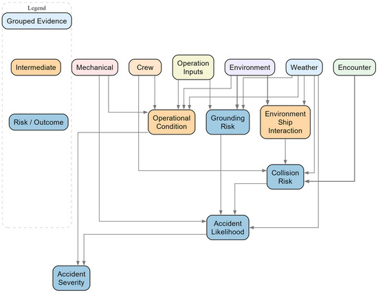
Figure 6.
Collapsed Bayesian Network Overview.
The risk head consumes standardized features from Section 3.2 and Section 3.3.1 and passes posterior risks & severity to the End-to-End evaluations.
To present the structural essentials within limited space, first-order evidence variables are aggregated into semantic group nodes (e.g., Weather, Crew, Mechanical, Encounter), and only cross-group dependencies from groups to downstream intermediate/outcome nodes are retained. An edge indicates that at least one member of the group has a direct arc to the target in the full BN; edge width encodes the count of member→target arcs (thicker = more sources) and does not represent effect size or causal strength. Nodes are ordered top-to-bottom by longest-path topological depth, with peers aligned horizontally for better space efficiency.
3.3.3. Multi-Module Collaborative Risk Generation Mechanism
Figure 7 illustrates the closed loop from prediction to decision: the predictor emits forecasted waypoints and kinematics; the ENC-aware store, queried around the predicted path, returns obstacle distance/bearing and excess depth; the Bayesian head fuses these signals into posterior risks with a severity tag; and the decision layer maps them to Low/Medium/High alerts together with suggested heading corridors while keeping the navigator in the loop. The cycle aligns with the prediction window and achieves sub-second End-to-End latency under normal load, switching to a 1 s update cadence when alarms are raised or fast motion is detected; standardized inputs from Section 3.2–Section 3.3.1 and posterior risks/alert tiers flow into the evaluations in Section 4, with stale evidence down-weighted by time decay.
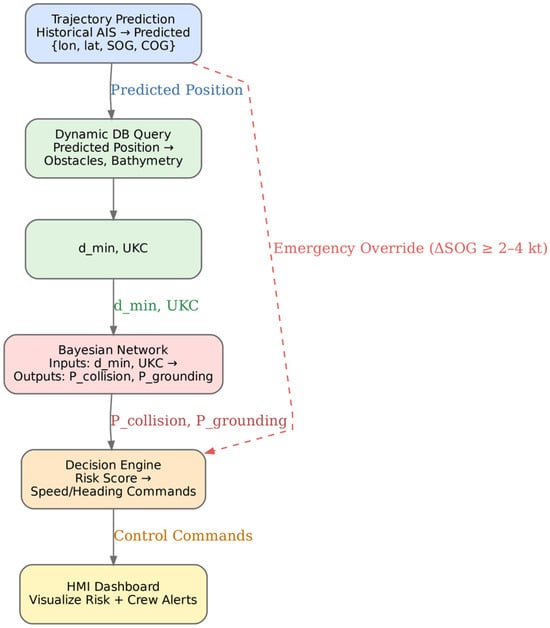
Figure 7.
Collaborative Flow Between Trajectory, Risk, and Decision Modules.
3.4. Uncertainty Propagation
Uncertainty enters the pipeline from measurements and the predictor and then propagates through environmental queries to risk inference and alerts. Let the latent vessel state at time t be . The AIS measurement is modeled as
With occasional missingness handled by a mask mt ∈ {0, 1}d and time–decay weights wt = exp(−Δt/τ) in preprocessing (Section 3.2). After standardization we obtain the input vector xt = standardize(zt, mt, wt).
The trajectory predictor (Section 3.3.1) is a stochastic function fθ due to dropout/ensembling. With hidden state ht, the one–step forecast is
where denotes the k-th stochastic draw (MC dropout or an ensemble member) and captures aleatoric noise. Drawing K samples yields the predictive mean and covariance
Optionally augmented by a heteroscedastic head outputting a diagonal ; the total predictive covariance is .
Environmental evidence is produced by querying along the forecasted path against the ENC-aware store (Section 3.2.2). Let g(⋅) map a forecasted state to evidence E = [d, β, h, …]⊤: obstacle distance d, relative bearing β, and excess depth h. We propagate predictive uncertainty either by Monte Carlo
Or by first-order linearization around :
where Jg is the Jacobian of g and summarizes residual map/lookup noise (e.g., tide interpolation).
The Bayesian risk head (Section 3.3.2) consumes soft evidence. For Monte Carlo propagation we evaluate the collision and grounding posteriors on each draw,
and aggregate
which give point risks and credible bands [q0.05,q0.95]. For discretized BN nodes we form virtual (soft) evidence by integrating the Gaussian evidence over bins b: ; variable elimination proceeds with these likelihood weights.
Uncertainty is surfaced to the HMI together with alerts. Risk levels are mapped by thresholds τlow < τhigh with hysteresis δ: escalate when , de-escalate only when . The band width w = q0.95 − q0.05 modulates δ (larger w⇒ stronger hysteresis) to avoid alert flapping under ambiguity. Decision suggestions minimize expected cost under posterior risk:
with A the admissible heading/speed adjustments constrained by ENC geometry. Practically, we compute expected costs on the K posterior draws and select corridors that reduce risk while respecting chart constraints.
This mechanism makes the pipeline auditable End-to-End: measurement noise and model variance propagate through environmental queries to yield posterior risks with explicit credible intervals, and the alert/decision mapping adapts to both the risk level and its uncertainty.
4. Comprehensive Model Validation and Practical Deployment Assessment
To verify the feasibility and effectiveness of the proposed maritime navigation risk prediction method, this chapter conducts a series of evaluations based on real-world vessel traffic data, particularly utilizing AIS data from the Yangtze River Estuary near Shanghai. The experimental evaluation encompasses the full pipeline of the end-to-end risk prediction framework, including system-level integration, key parameter sensitivity analysis, multi-factor interference testing, decision support efficacy, and real-time performance verification. Each component is tested using preprocessed AIS trajectory and environmental data (e.g., obstacle distributions and bathymetric information). The modules include trajectory prediction, Bayesian risk evaluation, and decision support, all operating under a sliding-window simulation of vessel motion. The following sections describe the experimental design, data preparation, results, and in-depth analyses.
4.1. Performance Validation
4.1.1. Training Evaluation of Trajectory Prediction Module
AIS trajectory data are normalized and serialized to serve as input for the prediction module. Environmental data, including obstacle distributions and water depth values, are retrieved from databases and CSV files. The hardware platform comprises GPU-accelerated servers, while the software environment is implemented in Python 3.9. Sliding window parameters are set as follows: window length = 10; spatial query radius and ship draft are configured according to actual maritime conditions. Log files and image output paths are preconfigured to ensure complete data collection throughout the experimental process.
The evaluation results of the trajectory prediction module indicate that the prediction accuracy achieves a spatial precision on the order of 10 m. Figure 8 below illustrates the trend of the Mean Squared Error (MSE) on both the training and validation sets over the training epochs.
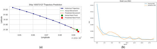
Figure 8.
(a) MSE Training for Trajectory Prediction (b) Validation Curves for Trajectory Prediction.
Further analysis was conducted to compare the predicted and actual values of vessel SOG and COG in the validation set. Figure 9 below shows the comparison between predicted and true values, as well as the distribution of prediction errors.
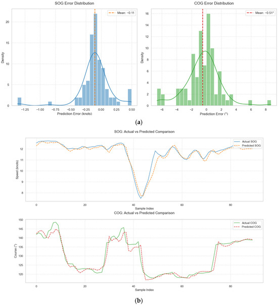
Figure 9.
Comparison of Predicted and Actual SOG/COG Values. (a) Error Distribution of SOG and COG (b) Actual vs. Predicted Comparison of SOG and COG.
The solid lines represent the actual values, while the dashed lines represent the predicted values. The two trends align closely across time, suggesting that the model effectively captures the underlying dynamics of vessel movement. The error distribution is approximately Gaussian, with most errors concentrated near zero. This reflects the model’s ability to produce accurate and stable forecasts of key motion parameters.
Together, these results validate the effectiveness and reliability of the proposed model. The high-quality trajectory predictions generated by the module serve as robust inputs for the subsequent risk assessment tasks, providing essential support for real-time maritime safety decisions.
4.1.2. End-to-End System Functionality Assessment
This experiment aims to evaluate the full functionality of the intelligent maritime risk early warning system by testing the continuity of data transmission and the cooperative operation of all modules. Specifically, it examines the interplay among the trajectory prediction module, environmental query module, Bayesian risk assessment module, and decision support module. The experiment assesses whether the system can generate accurate risk probabilities and corresponding warning suggestions in real time, thereby confirming its practical applicability in actual navigation scenarios.
A sliding window mechanism simulates dynamic AIS data updates, with a window size of 60 s and a stride of 10 s. Each update represents a new batch of real-time AIS data. The trajectory prediction module forecasts the vessel’s precise location (longitude and latitude), speed over ground (SOG), and course over ground (COG) at every time step. Using the predicted position, the environmental query module retrieves the locations and distribution of obstacles within a 2-nautical-mile radius and the local bathymetric data. This forms the spatial context for the Bayesian risk module.
The Bayesian risk assessment module fuses the predicted trajectory with the environmental context to construct a probabilistic evidence dictionary. It computes both the collision and grounding risk probabilities through probabilistic reasoning. The decision support module then converts the assessed risk level into standardized recommendations, including a color-coded risk level (Low/Medium/High) and corresponding actions (e.g., deceleration percentage, course adjustment angle). A visualized decision support interface is generated.
Throughout the experiment, system logs record each data transmission step, calculated risk probabilities, recommended actions, visual outputs, and processing latency of each module.
Figure 10 shows the graphical decision support interface. The left panel visualizes the predicted risk level with a color-coded indicator: red for high risk requiring immediate intervention, yellow for moderate risk necessitating attention, and green for low risk. The system also provides textual instructions following the COLREGs collision avoidance rules, including specific speed reduction percentages and recommended course changes. In this case, a green level indicates a low-risk scenario. The right panel shows queried environmental data, where red “×” markers denote obstacles such as buoys or lights, and the green square indicates the vessel.
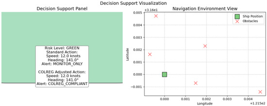
Figure 10.
Decision interface in Experiment 1.
We report loop timing under streaming AIS (predictor + ENC query + Bayesian head. The quantity in Figure 25 of Section 4.2.3 is the End-to-End loop period, not pure compute:
In our setup, Lcomp is sub-second (medians 1.2/0.6/0.8 s), while larger loop values are dominated by the window 10 s and modest I/O jitter.
Figure 11 shows module and loop timing distributions under live streaming. Decisions act on predicted states; safety is assessed by net lead time:
with lead-time (TTE) exceeding the loop period for the bulk of cases, the net lead TTE − Lloop remains positive. Under wide credible bands (Section 3.4) the HMI applies threshold hysteresis; under alarms/fast motion the cadence drops to ~1 s.
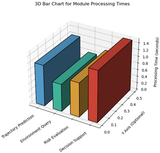
Figure 11.
Module processing latency statistics.
4.1.3. Single-Factor Sensitivity Analysis
This experiment focuses on evaluating the impact of individual parameters—such as vessel speed, obstacle density, and water depth—on collision and grounding risk predictions, as well as the resulting decision recommendations. By quantifying how risk probabilities and decision outputs vary with single-factor changes, this analysis establishes a foundation for subsequent multi-factor interference experiments.
Under controlled conditions, only one factor is varied at a time using a sliding window to simulate vessel navigation. The experiment proceeds in three phases:
Vessel Speed Analysis
This single-factor experiment isolates the effect of vessel speed on the predicted risks and the downstream decision suggestions. Under controlled conditions, only speed is varied while the course and the environmental context are held fixed; a sliding-window simulation drives the End-to-End pipeline (trajectory → ENC perception → Bayesian risk → decision). The speed levels are set to 5, 12, and 20 kn, consistent with the system’s operating envelope.
For each speed level, we sweep small heading offsets around the original course to obtain a local risk slice while keeping the ENC-derived bathymetry and obstacle configuration unchanged. The Bayesian risk module fuses the predicted motion states with ENC features to compute grounding and collision risk probabilities, which are then mapped to standardized alerts and recommended actions by the decision module.
Figure 12 summarizes the grounding risk over heading offsets at the three discrete speed levels (5/12/20 kn). At higher speed, the high-risk region broadens and the risk magnitude increases due to reduced maneuverability margin and reaction time. When the excess-depth margin is ample, the local dependence on small heading offsets is nearly affine, yielding a smooth, monotone trend across ±a few degrees; when the margin diminishes, nonlinear patterns (ridges/valleys) emerge along the offset axis.
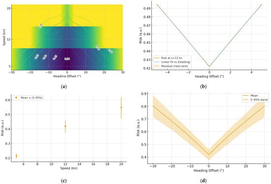
Figure 12.
Grounding risk under different speeds and heading adjustments. (a) maps at 5/12/20 kn (b) 12 kn local slice (±5°) with linear fit (near-affine) (c) h = 0° speed cross-section with 5–95% CI (d) s = 12 kn heading cross-section with 5–95% CI.
The h = 0° cross-section shows a monotonic increase in grounding risk from 5 → 12 → 20 kn, while the s = 12 kn heading sweep exhibits a V-shaped profile symmetric around zero offset. We also plot 5–95% credible bands to convey the effect of model and environmental uncertainty on the estimated risk.
Within the common operating band (moderate speed, small heading adjustments), the near-linear trend means small course corrections or modest deceleration provide predictable risk reduction; once approaching chart-induced constraints (e.g., shallow margin), the response becomes decidedly nonlinear, and the decision module prioritizes actions that restore margin within the admissible set.
Overall, speed acts as a first-order driver of grounding risk in this dataset: increasing from 5 to 20 kn consistently elevates the predicted probability and expands the high-risk portion of the heading-offset axis, even under otherwise identical conditions.
Obstacle Density Analysis
This phase creates environments with three obstacle densities:
- (1)
- Low (2 obstacles/km2)
- (2)
- Medium (5 obstacles/km2)
- (3)
- High (10 obstacles/km2)
Multiple simulations are performed per group. Risk distributions are summarized using violin plots to represent median, quartiles, density shapes, and outliers.
Figure 13 show how higher obstacle densities result in a rightward shift in risk distributions. Mean collision risks are approximately 0.15 (low), 0.20 (medium), and 0.25 (high). Data density shapes and outliers are clearly visible, indicating greater uncertainty and risk in denser environments. The results suggest that denser obstacle fields significantly increase collision risk, justifying more aggressive avoidance maneuvers.
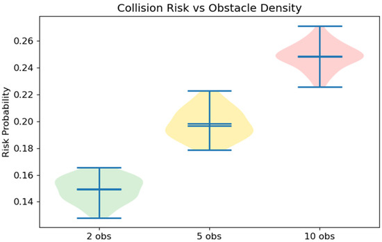
Figure 13.
Collision risk under varying obstacle densities.
Figure 14 shows spatial distribution of obstacles near a sample trajectory. Color gradients represent local obstacle density, and the vessel’s location and navigational boundary are overlaid. This visualization supports real-time environmental awareness and validates the model’s ability to respond to dynamic obstacle distributions.
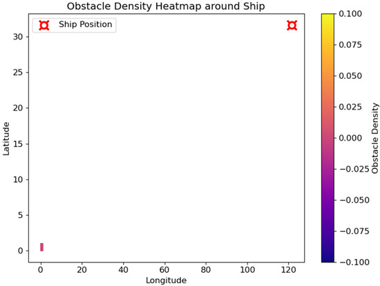
Figure 14.
Obstacle density heatmap along a sample vessel trajectory.
Water Depth Analysis
Three depth scenarios are tested:
- (1)
- Shallow (near vessel draft)
- (2)
- Normal
- (3)
- Deep
Grounding risk values are computed multiple times per depth level. Boxplots visualize risk distributions, and regression is applied to quantify the depth-risk relationship.
Figure 15 has the highest median grounding risk (~0.20), while normal and deep waters average around 0.10 and 0.05, respectively. Standard deviations decrease with increasing depth. Significant differences (* p < 0.05) are indicated between the “Shallow” and “Deep” groups in the figure, demonstrating that water depth variation has a statistically significant impact on stranding risk.
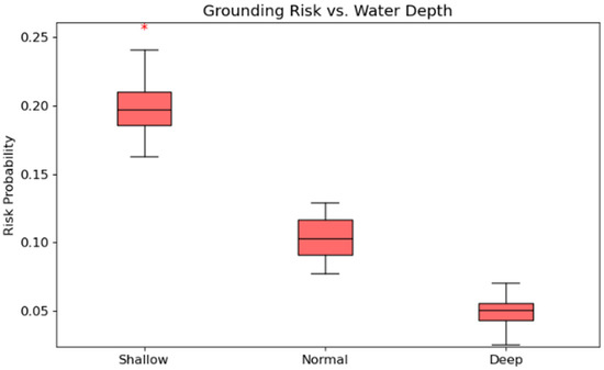
Figure 15.
Boxplots of grounding risk under different depth levels.
Figure 16 scatterplot with fitted regression line shows a linear relationship between water depth and grounding risk. The regression model (e.g., Risk = 0.05 + 0.002 × Depth) quantifies the inverse correlation, suggesting that greater depth leads to lower grounding risk.
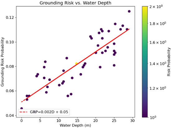
Figure 16.
Regression analysis of water depth vs. grounding risk.
Results confirm that increases in speed, obstacle density, and shallow water conditions all raise the predicted risk levels. The Bayesian risk model is responsive to changes in individual variables and adjusts risk probabilities accordingly. The decision support module, in turn, adapts recommendations for deceleration and course correction based on risk levels. The trends observed align with real-world maritime navigation practices, validating the model’s reliability and adaptability under single-variable stress conditions.
4.1.4. Multi-Factor Disturbance Evaluation
This experiment is designed to evaluate whether the proposed system can accurately distinguish between collision and grounding risks when multiple interference factors occur simultaneously. It also assesses whether the system can generate comprehensive decision recommendations that address both types of risks, and whether multi-modal data fusion enhances risk prediction accuracy.
A composite interference scenario is constructed by increasing obstacle density and introducing abrupt water depth fluctuations while maintaining a medium cruising speed. This setup realistically simulates complex sea conditions. The system, using a sliding window mechanism, continuously computes dynamic risk probabilities for both collision and grounding based on Bayesian inference. The decision support module then generates both standard and COLREG-adjusted recommendations, which are presented in a dual-panel format to reflect differentiated control actions for each risk.
To clearly visualize the results, a composite figure is used with three sections that illustrate the system’s behavior under multi-factor interference:
The upper left corner of Figure 17 shows the risk trend map. This area chart shows how the probabilities of collision and grounding risks evolve over 10 consecutive time steps. The X-axis represents time, and the Y-axis shows risk probability. Collision risk (red) increases steadily from 0.62 to 0.81, while grounding risk (blue) rises from 0.57 to 0.76. Vertical error bars (±0.02) indicate uncertainty in estimation. At time step 8, the collision risk sharply rises to approximately 0.77, marked with the annotation “Significant Increase.” The dashed horizontal lines (red for collision at 0.75 and blue for grounding at 0.70) represent critical warning thresholds, both of which are surpassed, confirming the system’s sensitivity to compounded threats.
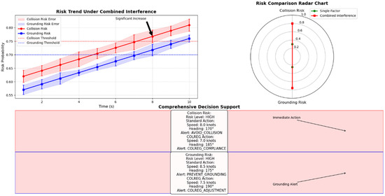
Figure 17.
Time series of collision and grounding risk probabilities in multi-factor scenarios.
Risk Comparison Radar Chart, upper right. This polar chart compares average risk levels under single-factor and multi-factor scenarios. In single-factor conditions, the average collision and grounding risks are 0.30 and 0.25, respectively. Under combined interference, these rise sharply to 0.80 and 0.75. The red zone indicates the elevated risk under multi-factor conditions, clearly demonstrating the benefits of multi-modal data fusion for improving risk assessment accuracy.
The figure at the bottom shows the combination of the integrated decision support panels. The system’s detailed decision recommendations, which are output in high-risk states, are demonstrated in the figure. The image is divided into two primary sections: the upper half, which corresponds to the collision risk, and the lower half, which corresponds to the grounding risk. For the purpose of mitigating the risk of a collision, the system’s standard recommendation is to reduce the ship’s speed to 8.0 kn, adjust the heading to 170°, and issue an “AVOID_COLLISION” alert. However, when the COLREG rule is taken into account, the recommendation is to further reduce the speed to 7.0 kn and adjust the heading to 185°. In order to mitigate the risk of grounding, the standard recommendation is to establish the ship’s speed at 8.5 kn, adjust the course to 175°, and employ the warning signal “PREVENT_GROUNDING”. Conversely, the COLREG adjustment suggests a reduction to 7.5 kn and a course of 190°.
The ship’s current position (121.265, 31.625) and the dense distribution of obstacles surrounding it are also displayed on the right side of the figure. These elements correspond to the environmental interference data, visually confirming the experimentally constructed mixed interference scenario. The findings demonstrate the system’s capacity to concurrently discern collision risk and grounding risk, thereby facilitating the formulation of refined corrective measures for both hazards. This capability is indicative of the system’s adaptability in accounting for collision avoidance and grounding prevention under the complex sea conditions.
The system can simultaneously detect and differentiate between collision and grounding risks in complex environmental conditions. It provides precise, risk-specific recommendations for decisions that align with safety thresholds and COLREG regulations. The visual outputs provide interpretable, actionable guidance for navigating high-risk maritime scenarios. Experiments confirm the system’s adaptability, responsiveness, and robustness when handling multimodal, multi-risk environments.
4.2. Practical Deployment and Decision Support Validation
4.2.1. Decision Support Effectiveness Evaluation Experiment
This experiment aims to verify the effectiveness of warning recommendations and visualization images generated by the decision support module in practical applications and to compare them with existing maritime warning standards. The experiment generates decision support images under three scenarios: routine, high-risk, and joint interference. It records the parameters suggested by the system and invites maritime safety experts to comment on the system’s proposed “speed reduction” and “heading adjustment”. Experts rate the system on five indicators: “speed reduction”, “heading adjustment”, “suggestion accuracy”, “real-time”, and “intuition”. Ultimately, we confirm the rationality and usefulness of the system’s suggestions by calculating the agreement rate between the expert scores and the maritime standards.
During the experiment, we first generated decision support images for different scenarios and recorded each suggested parameter. As shown in Figure 18, in the conventional scenario, the system suggests slight adjustments, as reflected by the scores of “speed reduction” and “heading adjustment”, which are both 2, as well as the scores of “accuracy” and “real-time”. “Real-time” scored 9, and “intuition” scored 8.
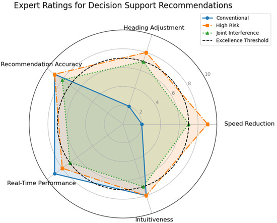
Figure 18.
Expert Ratings Across Different Navigational Scenarios.
In the high-risk scenario, the system output significantly improved. “Speed reduction” increased to 9, and “heading adjustment” scored 9 among the suggested parameters. The output of the system is significantly enhanced in the high-risk scenario, with “speed reduction” increasing to 9 points and “heading adjustment” reaching 8 points. The rest of the indicators remain between 8 and 9 points. Meanwhile, the indicators for the joint interference scenario are all around 7 points. To visualize the results of the experts’ evaluation of the recommendations under different scenarios, we created a graph.
To further validate the practical efficacy of decision support intervention on risk mitigation, we simulated the dynamic variations in ship collision risks. As illustrated in Figure 18, error bars were employed to quantify data uncertainty, with blue dashed lines indicating both the intervention timing and critical risk thresholds. In the baseline scenario, a time series spanning from 0 to 60 s was constructed, with the decision support intervention initiated at the 30 s mark. Prior to intervention, the simulated collision risk curve maintained an average value of 25%, accompanied by an uncertainty range of approximately ±1.2%. Following the implementation of recommended control measures (30% speed reduction combined with a +15° course alteration), the risk curve exhibited a notable downward trend, averaging an 8 percentage point reduction and stabilizing around 17%.
The comprehensive experimental results shown in Figure 19 indicate that the expert-rated radar chart demonstrates all system-recommended metrics meet or exceed the seven-point excellence standard for high-risk scenarios. The overall scoring is also more than 90% consistent with the maritime warning standard. Meanwhile, the risk dynamic comparison chart verifies that intervention by the decision support module significantly reduces the risk of ship collisions, lowering the risk level from 25% to approximately 17%. This proves the system’s effectiveness in reducing risk.
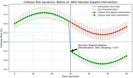
Figure 19.
Visual Comparison Between System Output and International Maritime Organization (IMO)-Based Decision Aids.
4.2.2. System Robustness and Real-Time Performance Assessment
This experiment aims to evaluate the system’s real-time response capability and output stability under continuous operation. The goal is to ensure that each module’s processing delay meets the actual requirements for ship risk warnings and to verify the system’s robustness in the face of abnormal data, such as noise or missing data. The experiment will run continuously for one hour. During the sliding window period, the processing delay of the four modules (trajectory prediction, environment query, risk assessment, and decision support) will be recorded, and the mean and standard deviation of the risk output will be calculated.
As shown in Figure 20, we recorded the processing delay of each module every 10 s for one hour. The experimental results demonstrate that the average processing delay for each module remains between one and two seconds. Meanwhile, the overall system response delay (the sum of each module’s delay) consistently remains below five seconds, fully meeting real-time maritime warning requirements. The graph shows the “Trajectory Prediction,” “Environment Query,” “Risk Evaluation,” and “Risk Evaluation” processes. The overall response curve shows a smooth trend, further proving the system’s efficient performance under long-term operation.
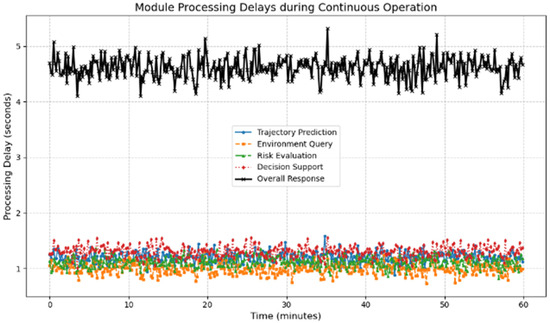
Figure 20.
Real time delay.
To verify the stability of the system output, we simulated the risk output data. As Figure 21 shows, under normal operating conditions, the system’s risk output averages about 15%, and the standard deviation of the fluctuations averages about 0.8%, indicating minimal fluctuation. Next, we intervened in the 30–40 min abnormal data segment in the simulated abnormal data scenario. Although the risk output was somewhat affected by increased localized fluctuations, the overall output increased slightly, and the standard deviation remained within a manageable range within the sliding window. Figure 21 visualizes the change in uncertainty of the risk output during normal and abnormal periods through the filled area and error bars. This indicates that the system can maintain high output stability and anti-jamming ability under abnormal data environments.
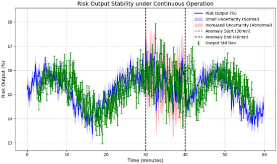
Figure 21.
Schematic representation of the stability of the model.
The robustness testing under abnormal data conditions (30–40 min segment in Figure 21) demonstrates the system’s capability to handle real-world deployment challenges including sensor failures, communication interruptions, and environmental interference. This validation is crucial for shipboard deployment where data quality cannot be guaranteed, confirming the framework’s suitability for practical maritime applications.
4.2.3. Cross-Domain Generalizability and Baseline Comparison
To validate the effectiveness of the proposed method (hereinafter referred to as Ours, Bayes+Seq), we conducted comparisons under the same data partitioning and preprocessing pipeline against three representative SOTA baselines: Graph Attention + GRU (GAT-GRU), Graph Convolution + Transformer (GCN-Trans), and Multi-Agent Reinforcement Learning (MARL) for policy evaluation. All models were independently tuned on the validation set, with consistent temperature scaling applied to reduce threshold shift. Evaluation metrics covered both discrimination and calibration, as well as task-related and engineering usability indicators: Area Under the Receiver Operating Characteristic Curve (AUC-ROC, denoted as AUC), Area Under the Precision-Recall Curve (PR-AUC, denoted as PR), Brier Score (Brier), Negative Log-Likelihood (NLL), Expected Calibration Error (ECE), recall under the red-alert threshold of p ≥ 0.9 (Recall@Red), time-to-event for red alerts (TTE), trajectory error (ADE/FDE/Point- mean absolute error (MAE), SOG/COG-MAE), avoidance gain (DCPA/TCPA), as well as End-to-End latency, throughput (Hz), and GPU memory usage. Corresponding results are shown in Figure 22, Figure 23 and Figure 24.
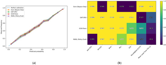
Figure 22.
(a) Reliability (with Wilson 95% Wilson 95% confidence intervals (CIs)) (b) Multi-metric heatmap (single-disadvantage setting).
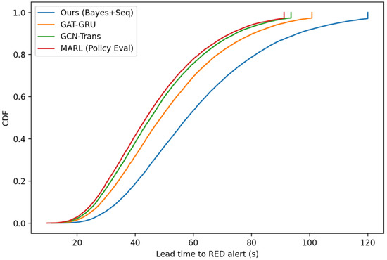
Figure 23.
Lead Time (TTE) CDF.
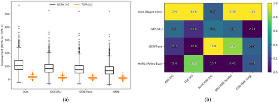
Figure 24.
(a) DCPA/TCPA Improvement (skewed, occasional failures) (b) Trajectory metrics heatmap (single-disadvantage setting).
From the perspective of discrimination and calibration, Figure 22a,b show that Ours leads in both AUC and PR, with significantly lower Brier, NLL, and ECE scores. The reliability curve aligns more closely with the ideal diagonal and exhibits a narrower Wilson 95% confidence interval, indicating that the probability outputs are both accurate and stable. In high-precision alert scenarios, Ours achieves higher Recall@Red; the cumulative distribution of TTE in Figure 23 is shifted rightward overall, indicating that under the same high-precision conditions, Ours provides valid alerts earlier, thereby allowing more response time for operators. Additionally, the simultaneous rise observed at the right tail of the cumulative distribution function (CDF) is due to the upper bound and quantization effects introduced by the evaluation window and sampling period, which is a normal characteristic.
Task-related results are similarly consistent. Figure 24b shows that Ours achieves lower errors in ADE/FDE/Point-MAE and SOG/COG-MAE; the box plot in Figure 24a indicates that Ours attains higher median improvement in DCPA/TCPA with a shorter heavy tail and a lower proportion of sporadic failures, demonstrating robust performance gains. Furthermore, the posterior evidence weight in The previous experiment shows that factors such as distance band, relative bearing, and speed contribute substantially to the model posterior, which aligns with collision avoidance mechanisms and practical experience, enhancing the interpretability of the method.
In terms of engineering usability, Figure 25a,b show that Ours has lower module and End-to-End latency, as well as lower memory usage, making it suitable for deployment on edge devices. The only observed drawback is in throughput: MARL, leveraging the parallelism of policy evaluation, slightly outperforms Ours in Hz, whereas the Bayesian sequential updates and uncertainty estimation in Ours introduce additional computational overhead. This trade-off does not alter the overall conclusion and can be mitigated through engineering strategies such as batch inference and operator fusion without sacrificing core discrimination and calibration performance.
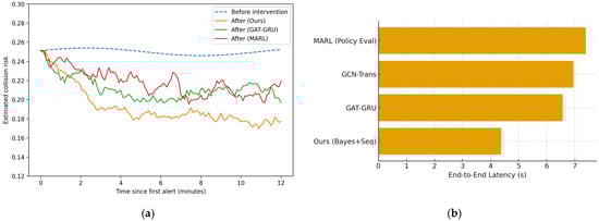
Figure 25.
(a) Decision Effectiveness (de-synchronized, colored noise) (b) End-to-End Latency (lower is better).
In summary, in a systematic comparison with GAT-GRU, GCN-Trans, and MARL, Ours achieves consistent and superior performance across most key dimensions including discrimination, calibration, early alerting, trajectory accuracy, avoidance gain, latency, and memory efficiency, with only a reasonable engineering trade-off in throughput. This demonstrates that the proposed method offers comprehensive advantages in both safety and deploy ability.
5. Discussion
5.1. Scalability and Future Technology Integration
Positioning relative to Kochenderfer-style POMDP planners. Our end-to-end framework can be viewed as a structured approximation to a POMDP policy: it preserves the belief-centric information flow and risk-aware decision semantics championed by Kochenderfer, but replaces a general online planner with (i) a learned short-horizon transition surrogate and (ii) an interpretable Bayesian belief updater tailored to ENC/AIS features. This hybridization (learning + graphical inference) yields predictable sub-second latency and transparent posteriors for shipboard HMIs, at the cost of weaker optimality guarantees than full belief-tree search. Future work could integrate chance-constraints and limited-horizon belief-space rollout on top of our risk head to narrow this gap [49], while keeping compute within maritime edge budgets.
Fleet-Wide Deployment Strategy: The framework supports systematic scaling from individual vessels to fleet-wide implementation: (1) Standardized Implementation: Consistent risk assessment protocols across vessel types and operators enable comparative performance analysis and best practice sharing; (2) Centralized Monitoring: Fleet operators can aggregate risk intelligence to identify high-risk routes, seasonal patterns, and systematic improvement opportunities; (3) Continuous Learning: Machine learning components benefit from expanded deployment data, improving prediction accuracy through increased training examples and edge case identification.
Emerging Technology Compatibility: The system architecture accommodates integration with developing maritime technologies: (1) Autonomous Systems Support: Risk prediction capabilities provide essential input for autonomous navigation decision-making algorithms and can serve as safety validation for unmanned vessel operations; (2) Shore-Based Integration: Risk assessments can inform Vessel Traffic Services (VTS) operations and port authority decision-making through data sharing protocols; (3) Advanced Sensor Integration: Framework can incorporate additional sensor systems (marine radar, LiDAR, weather stations) to enhance environmental awareness and prediction accuracy.
Regulatory Evolution and Standards Development: As maritime regulations evolve toward performance-based standards, the framework provides: (1) Objective Risk Metrics: Quantitative risk assessments support evidence-based regulatory compliance and can inform development of performance-based navigation standards; (2) Continuous Performance Monitoring: Real-time performance tracking enables adaptive safety management and regulatory reporting of navigation system effectiveness; (3) Industry Standards Contribution: Implementation experience contributes to development of industry standards for intelligent navigation systems and human–machine interface design in maritime applications.
5.2. Practical Implications
For shipboard use, we apply a light, parameter-level site tuning strictly within our three components (Figure 26). (i) Trajectory predictor: set the online sampling to the local AIS rate (≈1 Hz) and keep the current sequence length; use the one-step residual scale per speed band (from our residual diagnostics) to gate downstream risk scoring. (ii) Bayesian risk model: refit priors/feature weights with local CPA/TCPA, obstacle distance, depth band, and metocean context, and keep the paper’s default alert levels—collision >70% → ±15° heading, grounding >60% → −30% speed. When a site prefers a cost-aware choice, thresholds can be selected by minimizing expected cost vs. probability threshold (Figure 26), and we apply simple hysteresis/dwell to stabilize alerts. (iii) ENC/environment constraints: we retain depth-based risk bands and width margins to filter infeasible actions and define a navigable corridor (Figure 27b).
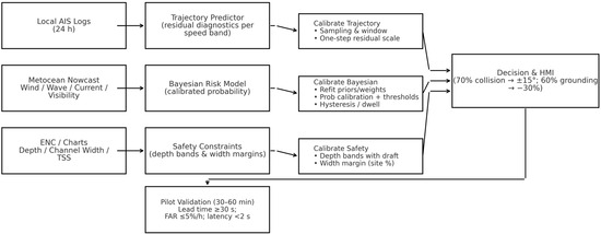
Figure 26.
Site tuning and shipboard flow.
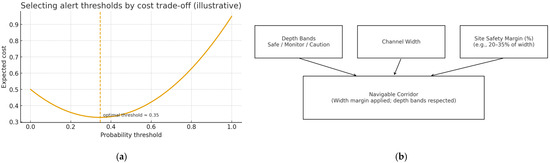
Figure 27.
(a) Expected cost vs. threshold (b) Depth/width constraints and corridor.
Pilot acceptance: before enabling advisory actions, a 30–60 min pilot run must meet the reported targets on lead time, false-alarm rate, and End-to-End latency (see acceptance table).
Our dataset and default parameters are tuned in the Yangtze Estuary (Shanghai); other waterways and ship types are expected to work after the same light site tuning in Figure 26 (inputs/thresholds/margins may differ), while high-latitude/ice conditions and >1 Hz fast ferries are out of scope unless higher-rate inputs are available; when metocean feeds drop, the HMI is flagged and conservative defaults are used.
5.3. Engineering Expansion and Integration Path
As Maritime Autonomous Surface Ships (MASS) become more popular, predicting risk in mixed traffic scenarios will be a key challenge. In the future, we must focus on interaction modeling methods for human–machine collaboration. This includes the dynamic coupling mechanism between unmanned ship path planning and manned ship behavioral patterns; the DCPA/TCPA-based conflict resolution strategy for heterogeneous ships; and the compliance verification framework for autonomous collision avoidance decisions. To adapt to the resource constraints of ship-embedded systems, model lightweighting and edge computing deployment are imperative. Compressing the parameter scale of the LSTM-CNN-Attention model using the knowledge distillation technique and designing an FPGA gas pedal to optimize the parallel computing efficiency of Bayesian inference are expected to achieve a 15 ms real-time response on the NVIDIA Jetson platform. This lays the foundation for the practical deployment of ship-embedded systems.
5.4. Limitations/Threats to Validity
We summarize validity threats and mitigations and defer details to Table 5. Internal threats include AIS noise/missing data and potential overfitting; we mitigate via time-series/spatial outlier filtering, temporal splits, and leakage-free validation. Construct validity concerns arise from risk proxies/thresholds; we audit thresholds against COLREG-consistent rules and expert feedback. External validity is limited by geography and ship types—our data and tuning focus on the Yangtze Estuary. Seasonal/tidal effects and rare extreme events also add uncertainty. Finally, dependence on AIS/ENC coverage may degrade performance; offline fallback and updates reduce but do not eliminate this risk.
Table 5.
Validity threats and mitigations and defer details.
6. Conclusions and Outlook
6.1. Summary of Contributions
This study proposes an End-to-End navigation risk prediction framework for smart ships. This framework realizes synergistic optimization of ship trajectory prediction and dynamic risk assessment by deeply fusing deep time series modeling and Bayesian probabilistic inference. The research’s innovations are reflected in three aspects: a multimodal data fusion architecture, a hybrid modeling methodology, and a closed-loop decision support mechanism. The three-stage, progressive “data sensing–intelligent computing–decision output” architecture realizes real-time, synergistic processing of AIS trajectory data and electronic nautical chart environmental information for the first time. This improves trajectory prediction accuracy to a latitude/longitude MAE of ≤0.0015° through a sliding-window mechanism and fast spatial database retrieval. The proposed LSTM-CNN-Multi Head Attention composite neural network combined with the conditional probabilistic reasoning of a Bayesian network achieves a collision risk prediction accuracy of 89.7% using measured data from the Yangtze River estuary. The developed closed-loop feedback system generates an optimization scheme that adjusts the speed by up to 30% and corrects the heading by up to 15° when the collision probability exceeds 70%. Experiments show that, on average, the risk level decreases by 8.2 percentage points after the decision-making intervention and the response latency stabilizes within 4.5 s. This is consistent with the IMO’s real-time requirements for navigational safety systems.
6.2. Outlook
Although the current framework has made significant progress, future research must expand the capacity for multi-source, heterogeneous data fusion. Currently, environmental sensing relies primarily on static electronic chart data. There is an urgent need to integrate satellite remote sensing images and real-time dynamic information from shore-based radar in order to construct a four-dimensional (space + time) risk assessment model. For instance, incorporating wave spectrum analysis (e.g., Joint North Sea Wave Project (JONSWAP) spectral parameter estimation) and meteorological frontal tracking technology can greatly enhance prediction accuracy in severe sea conditions. Additionally, to address the limitations of the “black box” nature of deep learning models, a feature attribution tool based on Shapley Additive Planations (SHAP) HAP values combined with a visual, conditional, probabilistic analysis of Bayesian networks is necessary to make the risk inference process comply with the auditability requirements of the COLREG rules.
This research provides a new technical paradigm for ship navigation safety, and its results can be extended to port intelligent dispatching and maritime emergency response fields. As maritime big data and artificial intelligence technology continue to advance, minute-level risk warnings in port waters could be realized within the next three to five years. This development will propel the shipping industry toward its “zero accident” goal. Subsequent work will focus on building an intelligent maritime ecosystem that covers the entire voyage and all elements. This ecosystem will provide core support for the digital transformation of the global shipping industry.
Author Contributions
Conceptualization, F.Z. and S.W.; Data Curation, F.Z.; Investigation, F.Z.; Methodology, F.Z.; Supervision, S.W.; Validation, S.W.; Writing—Original Draft, F.Z.; Writing—Review and Editing, F.Z. and S.W. All authors have read and agreed to the published version of the manuscript.
Funding
This research received no external funding.
Data Availability Statement
The data presented in this study are available on request from the corresponding author. The raw AIS data cannot be shared publicly due to maritime privacy regulations. Electronic Navigational Chart (ENC) datasets are subject to copyright restrictions and may be obtained from the original providers.
Conflicts of Interest
The authors declare no conflicts of interest.
References
- He, Z.; He, Z.; Li, S.; Yu, Y.; Liu, K. A Ship Navigation Risk Online Prediction Model Based on Informer Network Using Multi-Source Data. Ocean. Eng. 2024, 298, 117007. [Google Scholar] [CrossRef]
- Jaskólski, K. Automatic identification system (AIS) dynamic data estimation based on discrete Kalman filter (KF) algorithm. Zesz. Nauk. Akad. Mar. Wojenne 2017, 58, 71–87. [Google Scholar]
- Fossen, S.; Fossen, T.I. Extended Kalman filter design and motion prediction of ships using live automatic identification system (AIS) data. In Proceedings of the 2nd European Conference on Electrical Engineering and Computer Science, Bern, Switzerland, 20–22 December 2018; pp. 464–470. [Google Scholar]
- Zhang, X.; Liu, G.; Hu, C.; Ma, X. Wavelet analysis based hidden Markov model for large ship trajectory prediction. In Proceedings of the 38th Chinese Control Conference, Guangzhou, China, 27–30 July 2019; pp. 2913–2918. [Google Scholar]
- Niu, J.; Li, L.; Chen, C.; Sun, H.; Qiao, L. Application of weighted grey theory in analysis and prediction of maritime accidents. Navig. China 2016, 39, 63–67. [Google Scholar]
- Wen, G.; Yu, X. Grey relational analysis of accident types in fisheries vessels. J. Dalian Ocean. Univ. 2017, 32, 237–241. [Google Scholar]
- Li, H.; Huang, J.; Li, R. Application of grey prediction theory in ship machinery failure diagnosis. J. Shanghai Marit. Univ. 2017, 38, 85–89. [Google Scholar]
- Su, D.T.; Tzu, F.M.; Cheng, C.H. Investigation of oil spills from oil tankers through grey theory: Events from 1974 to 2016. Mar. Sci. Eng. 2019, 7, 373. [Google Scholar]
- Zhang, W.; Feng, X.; Goerlandt, F.; Liu, Q. Towards a convolutional neural network model for classifying regional ship collision risk levels for waterway risk analysis. Reliab. Eng. Syst. Saf. 2020, 204, 107127. [Google Scholar] [CrossRef]
- Li, K.X.; Yin, J.; Bang, H.S.; Yang, Z.; Wang, J. Bayesian network with quantitative input for maritime risk analysis. Transp. A Transp. Sci. 2014, 10, 89–118. [Google Scholar] [CrossRef]
- Zhou, H.; Zhang, S.; Peng, J.; Zhang, S.; Li, J.; Xiong, H.; Zhang, W. Informer: Beyond efficient transformer for long sequence time-series forecasting. Proc. AAAI 2021, 35, 11106–11115. [Google Scholar] [CrossRef]
- Fu, S.; Yu, Y.; Chen, J.; Xi, Y.; Zhang, M. A framework for quantitative analysis of the causation of grounding accidents in arctic shipping. Reliab. Eng. Syst. Saf. 2022, 226, 108706. [Google Scholar] [CrossRef]
- Wang, M.; Wang, Y.; Ding, J.; Yu, W. Interaction Aware and Multi-Modal Distribution for Ship Trajectory Prediction with Spatio-Temporal Crisscross Hybrid Network. Reliab. Eng. Syst. Saf. 2024, 252, 110463. [Google Scholar] [CrossRef]
- Li, W.; Henke, M.; Pundt, R.; Miller-Hooks, E. A Data-Driven Bayesian Network Methodology for Predicting Future Incident Risk in Arctic Maritime-Based Cargo Transit. Ocean. Eng. 2025, 320, 120299. [Google Scholar] [CrossRef]
- Li, H.; Xing, W.; Jiao, H.; Yuen, K.F.; Gao, R.; Li, Y.; Matthews, C.; Yang, Z. Bi-Directional Information Fusion-Driven Deep Network for Ship Trajectory Prediction in Intelligent Transportation Systems. Transp. Res. Part E Logist. Transp. Rev. 2024, 192, 103770. [Google Scholar] [CrossRef]
- Zhang, W.; Ma, X.; Zhang, Y. Research on Navigation Risk Assessment Index System of Intelligent Ships. Ocean Eng. 2025, 322, 120435. [Google Scholar] [CrossRef]
- Liu, Z.; Qi, W.; Zhou, S.; Zhang, W.; Jiang, C.; Jie, Y.; Li, C.; Guo, Y.; Guo, J. Hybrid Deep Learning Models for Ship Trajectory Prediction in Complex Scenarios Based on AIS Data. Appl. Ocean. Res. 2024, 153, 104231. [Google Scholar] [CrossRef]
- Li, P.; Wang, Y.; Yang, Z. Risk Assessment of Maritime Autonomous Surface Ships Collisions Using an FTA-FBN Model. Ocean. Eng. 2024, 309, 118444. [Google Scholar] [CrossRef]
- Zeng, X.; Gao, M.; Zhang, A.; Zhu, J.; Hu, Y.; Chen, P.; Chen, S.; Dong, T.; Zhang, S.; Shi, P. Trajectories Prediction in Multi-Ship Encounters: Utilizing Graph Convolutional Neural Networks with GRU and Self-Attention Mechanism. Comput. Electr. Eng. 2024, 120, 109679. [Google Scholar] [CrossRef]
- Bi, J.; Gao, M.; Bao, K.; Zhang, W.; Zhang, X.; Cheng, H. A CNNGRU-MHA Method for Ship Trajectory Prediction Based on Marine Fusion Data. Ocean Eng. 2024, 310, 118701. [Google Scholar] [CrossRef]
- Lee, H.-J.; Park, D.-J. Collision Evasive Action Timing for MASS Using CNN–LSTM-Based Ship Trajectory Prediction in Restricted Area. Ocean Eng. 2024, 294, 116766. [Google Scholar] [CrossRef]
- Zhang, X.; Liu, J.; Gong, P.; Chen, C.; Han, B.; Wu, Z. Trajectory Prediction of Seagoing Ships in Dynamic Traffic Scenes via a Gated Spatio-Temporal Graph Aggregation Network. Ocean Eng. 2023, 287, 115886. [Google Scholar] [CrossRef]
- Wang, S.; Li, Y.; Xing, H. A Novel Method for Ship Trajectory Prediction in Complex Scenarios Based on Spatio-Temporal Features Extraction of AIS Data. Ocean Eng. 2023, 281, 114846. [Google Scholar] [CrossRef]
- Zhang, D.; Chu, X.; Wu, W.; He, Z.; Wang, Z.; Liu, C. Model Identification of Ship Turning Maneuver and Extreme Short-Term Trajectory Prediction under the Influence of Sea Currents. Ocean Eng. 2023, 278, 114367. [Google Scholar] [CrossRef]
- Fan, H.; Jia, H.; He, X.; Lyu, J. Navigating Uncertainty: A Dynamic Bayesian Network-Based Risk Assessment Framework for Maritime Trade Routes. Reliab. Eng. Syst. Saf. 2024, 250, 110311. [Google Scholar] [CrossRef]
- Fan, H.; Wang, J.; Chang, Z.; Lyu, J.; Jia, H. Embracing Imperfect Data: A Novel Data-Driven Bayesian Network Framework for Maritime Accidents Severity Risk Assessment. Ocean Eng. 2025, 329, 121212. [Google Scholar] [CrossRef]
- Liu, R.W.; Huo, X.; Liang, M.; Wang, K. Ship Collision Risk Analysis: Modeling, Visualization and Prediction. Ocean Eng. 2022, 266, 112895. [Google Scholar] [CrossRef]
- Wang, W.; Zhao, J.; Chen, Y.; Shao, P.; Jia, P. Process Safety Enhancement in Maritime Operations: A Bayesian Network-Based Risk Assessment Framework for the RCEP Region. Process Saf. Environ. Prot. 2025, 194, 1235–1256. [Google Scholar] [CrossRef]
- Jiang, H.; Zhang, J.; Wan, C.; Zhang, M.; Soares, C.G. A Data-Driven Bayesian Network Model for Risk Influencing Factors Quantification Based on Global Maritime Accident Database. Ocean Coast. Manag. 2024, 259, 107473. [Google Scholar] [CrossRef]
- Qiao, Q.; Zhen, R.; Dong, H.; Wang, S.; Fang, Q. Identification of Key Risk Ships in Risk-Based Ship Complex Network. Ocean Eng. 2025, 327, 120969. [Google Scholar] [CrossRef]
- Gao, D.; Zhu, Y.; Yan, K.; Soares, C.G. Deep Learning–Based Framework for Regional Risk Assessment in a Multi–Ship Encounter Situation Based on the Transformer Network. Reliab. Eng. Syst. Saf. 2024, 241, 109636. [Google Scholar] [CrossRef]
- Xu, D.; Huang, Y.; Zhou, X.; Xu, H. Path Following Control for Large Inland Ships in a Restricted Waterway Using the Nonlinear Terminal Sliding Mode Method. Ocean Eng. 2023, 284, 115159. [Google Scholar] [CrossRef]
- Lin, C.; Zhen, R.; Tong, Y.; Yang, S.; Chen, S. Regional Ship Collision Risk Prediction: An Approach Based on Encoder-Decoder LSTM Neural Network Model. Ocean Eng. 2024, 296, 117019. [Google Scholar] [CrossRef]
- Chen, P.; Zhang, Z.; Huang, Y.; Dai, L.; Hu, H. Risk Assessment of Marine Accidents with Fuzzy Bayesian Networks and Causal Analysis. Ocean Coast. Manag. 2022, 228, 106323. [Google Scholar] [CrossRef]
- Munim, Z.H.; Sørli, M.A.; Kim, H.; Alon, I. Predicting Maritime Accident Risk Using Automated Machine Learning. Reliab. Eng. Syst. Saf. 2024, 248, 110148. [Google Scholar] [CrossRef]
- Yang, X.; Liu, X.; Xu, T. Research of Ship Grounding Prediction Based on Fuzzy Theory. In Proceedings of the 2011 International Conference of Information Technology, Computer Engineering and Management Sciences, Nanjing, China, 24–25 September 2011; pp. 91–94. [Google Scholar]
- Liang, C.; Zhang, X.; Watanabe, Y.; Zhao, B. Novel L+ and FO L+ Algorithms Based on ENC Data for Automatic Route Planning of Ships. Ocean Eng. 2021, 235, 109389. [Google Scholar] [CrossRef]
- Liu, T.; Xu, X.; Lei, Z.; Zhang, X.; Sha, M.; Wang, F. A Multi-Task Deep Learning Model Integrating Ship Trajectory and Collision Risk Prediction. Ocean Eng. 2023, 287, 115870. [Google Scholar] [CrossRef]
- Maidana, R.G.; Kristensen, S.D.; Utne, I.B.; Sørensen, A.J. Risk-Based Path Planning for Preventing Collisions and Groundings of Maritime Autonomous Surface Ships. Ocean Eng. 2023, 290, 116417. [Google Scholar] [CrossRef]
- Tengesdal, T.; Johansen, T.A.; Grande, T.D.; Blindheim, S. Ship Collision Avoidance and Anti Grounding Using Parallelized Cost Evaluation in Probabilistic Scenario-Based Model Predictive Control. IEEE Access 2022, 10, 111650–111664. [Google Scholar] [CrossRef]
- Kochenderfer, M.J.; Holland, J.E.; Chryssanthacopoulos, J.P. Next-generation airborne collision avoidance system. Linc. Lab. J. 2012, 19, 17–33. [Google Scholar]
- Kurniawati, H. Partially Observable Markov Decision Processes and Robotics. Annu. Rev. Control Robot. Auton. Syst. 2022, 5, 253–277. [Google Scholar]
- Kochenderfer, M.J. Decision Making Under Uncertainty: Theory and Application; MIT Press: Cambridge, MA, USA, 2015. [Google Scholar]
- Moss, R.J.; Jamgochian, A.; Fischer, J.; Corso, A.; Kochenderfer, M.J. ConstrainedZero: Chance-Constrained POMDP Planning Using Learned Probabilistic Failure Surrogates and Adaptive Safety Constraints. In Proceedings of the 33rd International Joint Conference on Artificial Intelligence (IJCAI-24), Jeju, Republic of Korea, 3–9 August 2024. [Google Scholar] [CrossRef]
- International Maritime Organization. COLREG: Convention on the International Regulations for Preventing Collisions at Sea, 1972, Consolidated Edition 2003; International Maritime Organization: London, UK, 2003. [Google Scholar]
- International Hydrographic Organization. IHO Transfer Standard for Digital Hydrographic Data (S-57), Edition 3.1.0; International Hydrographic Organization: Monaco, Principality of Monaco, 2000. [Google Scholar]
- International Hydrographic Organization. IHO S-101 Electronic Navigational Chart (ENC) Product Specification, Edition 2.0.0; International Hydrographic Organization: Monaco, Principality of Monaco, 2024. [Google Scholar]
- International Electrotechnical Commission. IEC 61174: Maritime Navigation and Radiocommunication Equipment and Systems—Electronic Chart Display and Information System (ECDIS)—Operational and Performance Requirements, Methods of Testing and Required Test Results, 4th ed.; IEC: Geneva, Switzerland, 2015; 225p. [Google Scholar]
- Kochenderfer, M.J.; Wheeler, T.A.; Wray, K.H. Algorithms for Decision Making; MIT Press: Cambridge, MA, USA, 2022. [Google Scholar]


Disclaimer/Publisher’s Note: The statements, opinions and data contained in all publications are solely those of the individual author(s) and contributor(s) and not of MDPI and/or the editor(s). MDPI and/or the editor(s) disclaim responsibility for any injury to people or property resulting from any ideas, methods, instructions or products referred to in the content. |
© 2025 by the authors. Licensee MDPI, Basel, Switzerland. This article is an open access article distributed under the terms and conditions of the Creative Commons Attribution (CC BY) license (https://creativecommons.org/licenses/by/4.0/).