Causal Matrix Long Short-Term Memory Network for Interpretable Significant Wave Height Forecasting

Abstract

This study proposes a novel causality-structured matrix long short-term memory (C-mLSTM) model for significant wave height (SWH) forecasting. The framework incorporates a two-stage causal feature selection methodology using cointegration testing and Granger causality testing to identify long-term stable causal relationships among variables. These relationships are embedded within the C-mLSTM architecture, enabling the model to effectively capture both temporal dependencies and causal information within the data. Furthermore, the model integrates Bayesian optimization (BO) and twin delayed deep deterministic policy gradient (TD3) algorithms for synergistic optimization. This combined TD3-BO approach achieves an 11.11% improvement in the mean absolute percentage error (MAPE) on average compared to the base model without optimization. For 1–24 h SWH forecasts, the proposed TD3-BO-C-mLSTM outperforms the benchmark models TD3-BO-LSTM and TD3-BO-mLSTM in prediction accuracy. Finally, a Shapley additive explanations (SHAP) analysis was conducted on the input features of the BO-C-mLSTM model, which reveals interpretability patterns consistent with the two-stage causal feature selection methodology. This research demonstrates that integrating causal modeling with optimization strategies significantly enhances time-series forecasting performance.

1. Introduction

As a core element in the dynamic evolution of the upper ocean environment, ocean waves impact multiple domains, including the structural safety of marine engineering projects [1,2], efficient utilization of renewable energy [3,4], hydrodynamic performance optimization of vessels [5,6,7], and reliability assessment of marine disaster early-warning systems [8,9,10]. Wave forecasting primarily falls into two categories: conventional numerical modeling and machine learning approaches. Conventional numerical wave forecasting involves solving partial differential equations (i.e., wave action balance equations) on discrete grids based on wave spectrum evolution and responses to external forcing fields, such as wind, thereby achieving significant wave height (SWH) forecasts [11,12,13]. Through years of development, a multitude of numerical wave models have been established, encompassing the ECMWF Wave Model [14], the MASNUM Wave Model [15,16], the Simulating Waves Nearshore (SWAN) model [17], WaveWatch III (WW3) [18], and other prominent frameworks. However, the accuracy of numerical wave forecasting is constrained by incomplete understanding of wave-related physical mechanisms and numerical artifacts, such as Discrete Interaction Approximation [19] and the Garden Sprinkler Effect [20]. Furthermore, in coastal and nearshore regions, model accuracy is highly sensitive to the precision of input wind fields, bathymetric data, and boundary conditions [21].

The recent breakthroughs in artificial intelligence (AI) have expanded the methodological horizons for wave forecasting modeling. In particular, long short-term memory (LSTM) networks and their variants have been successfully applied to SWH prediction [21,22,23,24,25]. Fan et al. [26] developed a hybrid SWAN-LSTM model that integrates buoy observation data with the SWAN numerical model. Comparative results demonstrated that this approach improved SWH forecasting accuracy by over 65% compared to standalone SWAN simulations. Wang et al. [27] proposed an advanced wave forecasting model incorporating a convolutional neural network (CNN), bidirectional LSTM (BiLSTM), and an attention mechanism (CNN–BiLSTM–Attention), trained using WW3 reanalysis data. Under normal wave conditions, the model achieved root mean squared errors (RMSEs) of 0.063 m, 0.105 m, 0.172 m, and 0.281 m for 3, 6, 12, and 24 h forecasts, respectively. Additionally, LSTM has also been widely applied in other fields [28,29].

Beyond LSTM, a broader spectrum of machine learning techniques are increasingly being applied to oceanographic forecasting, demonstrating significant potential in capturing complex ocean dynamics. Graph Neural Networks (GNNs) have been employed to model complex spatial dependencies in ocean simulations, exemplified by hierarchical and adaptive architectures that serve as efficient surrogates for exploring the parameter space of unstructured-mesh models [30]. Hierarchical neural architectures offer another promising direction, facilitating multi-scale representation learning in hydrological perception models for underwater gliders [31] and global sea surface temperature (SST) prediction [32]. For probabilistic forecasting and uncertainty quantification, Gaussian Processes (GPs) provide a powerful framework, applied both in SST interpolation [33] and statistical modeling of ocean-wave data [34]. In a related context of hydrological forecasting, the effectiveness of machine learning models for daily streamflow prediction along with comprehensive uncertainty assessment has also been demonstrated, highlighting the broader potential of data-driven methods in environmental modeling [35]. Furthermore, novel hybrid models have emerged to address the coupled prediction of interrelated coastal hazards, such as joint forecasting of wave height and storm surge using deep learning approaches [36,37], enabling rapid and comprehensive hazard assessment over extended coastal regions.

Compared to conventional numerical forecasting models, AI-based approaches demonstrate significant advantages in both efficiency and accuracy for wave prediction. However, their widespread engineering application remains constrained by the inherent “black-box” nature of these models and associated interpretability challenges [38]. Dong et al. [39] demonstrated that incorporating prior knowledge of ocean dynamic processes into AI model architectures can simultaneously enhance both interpretability and forecasting precision. In a relevant methodological advancement, Li et al. [40] employed Pearson correlation analysis and Granger causality tests to identify causal relationships among predictive variables, subsequently embedding these relationships into an LSTM framework to create a causality-structured LSTM (C-LSTM) model for global soil moisture prediction across 64 monitoring stations. Their results showed that compared to standard LSTM, the C-LSTM achieved Nash–Sutcliffe efficiency improvements exceeding 10% at over 67% of the stations. Pushing this paradigm further, Wang and Jiang [13] developed a physics-guided deep learning model based on fundamental principles of wave dynamics, where wind waves are driven by local wind fields while swells propagate from distant wind systems. Their innovative approach used global 10 m wind vector fields from the preceding 240 h as input features to predict SWH, effectively bypassing the spectral computation limitations inherent in traditional numerical models.

These successful cases demonstrate the efficacy of physics-guided and causality-constrained deep learning approaches in earth system modeling. Building upon this foundation, we propose a novel causality-enhanced methodology for SWH prediction. First, we implement a two-stage causal feature selection framework employing cointegration tests and Granger causality tests. This systematically identifies dynamic coupling relationships between SWH and meteorological variables (wind speed, temperature, air pressure, etc.), subsequently constructing a causality-informed dataset. Then, a causal inference module is incorporated into the matrix LSTM (mLSTM) architecture to develop a causality-structured matrix LSTM (C-mLSTM) network. By integrating the causality-informed dataset with this causally constrained neural structure, a unified AI modeling framework is established to simultaneously enhance both interpretability and forecasting accuracy.

Considering that the performance of deep learning models is highly contingent upon hyperparameter selection, Bayesian optimization (BO) [41,42,43] is employed in this study to optimize the key hyperparameters of the C-mLSTM architecture. Additionally, to address the limitations of fixed time-window forecasting—in which critical information loss and outdated data interference may occur [44]—this work also implements an agent based on the twin delayed deep deterministic policy gradient algorithm (TD3) proposed by Fujimoto et al. [45]. This agent dynamically adjusts the input window length of the forecasting model based on historical data and historical prediction errors, enabling automatic optimization of temporal inputs according to evolving data patterns.

Building upon the advancements in causality-informed modeling, this study aims to develop a novel and interpretable deep learning framework for accurate and reliable SWH forecasting. The primary objectives are the following: (1) to design and implement a two-stage causal feature selection methodology for identifying stable, long-term drivers of SWH; (2) to construct a C-mLSTM architecture that effectively integrates these identified causal relationships to enhance both predictive performance and model interpretability; (3) to synergistically combine BO and a TD3 agent for automated hyperparameter tuning and dynamic input window adjustment, respectively, further optimizing the forecasting system’s accuracy and adaptability.

The paper is organized as follows: Section 2 describes the datasets, methodology, and model framework. Section 3 presents comparative results and a performance analysis. Section 4 discusses model sensitivity, interpretability, advantages, and limitations. Finally, Section 5 concludes the study.

2. Materials and Methods

2.1. National Data Buoy Center Dataset

Observational data from the National Data Buoy Center (NDBC), a division of the National Oceanic and Atmospheric Administration, are utilized in this research. Measurements are employed from two stations: Station 51000 in open-ocean waters (depth: 4762 m) and Station 46025 in nearshore waters (depth: 890 m), both with a temporal resolution of an hour (Figure 1). Key observed variables are detailed in

Table 1. The full names, abbreviations, and units of the variables.

Full Name	Abbreviation	Units
Air temperature	AT	K
Wind speed	WS	m/s
Wind direction	WD	Degree
Air pressure at sea level	AP	Pa
Sea surface temperature	SST	K
Average period	WP	s
Mean wave direction	MWD	Degree
Significant wave height	SWH	m

. Four years of continuous measurements (1 January 2019 to 31 December 2022) were acquired from both stations, with all data normalized prior to model training to accelerate model convergence. The normalization procedure is defined as follows:

$$x^{\ast }= {\displaystyle \frac{x- x_{min}}{x_{max}- x_{min}}}$$

(1)

where $x$ denotes the raw value in the time series; $x_{min}$ and $x_{max}$ represent the minimum and maximum values within the variable’s training set time series, respectively; and $x^{\ast }$ indicates the normalized value.

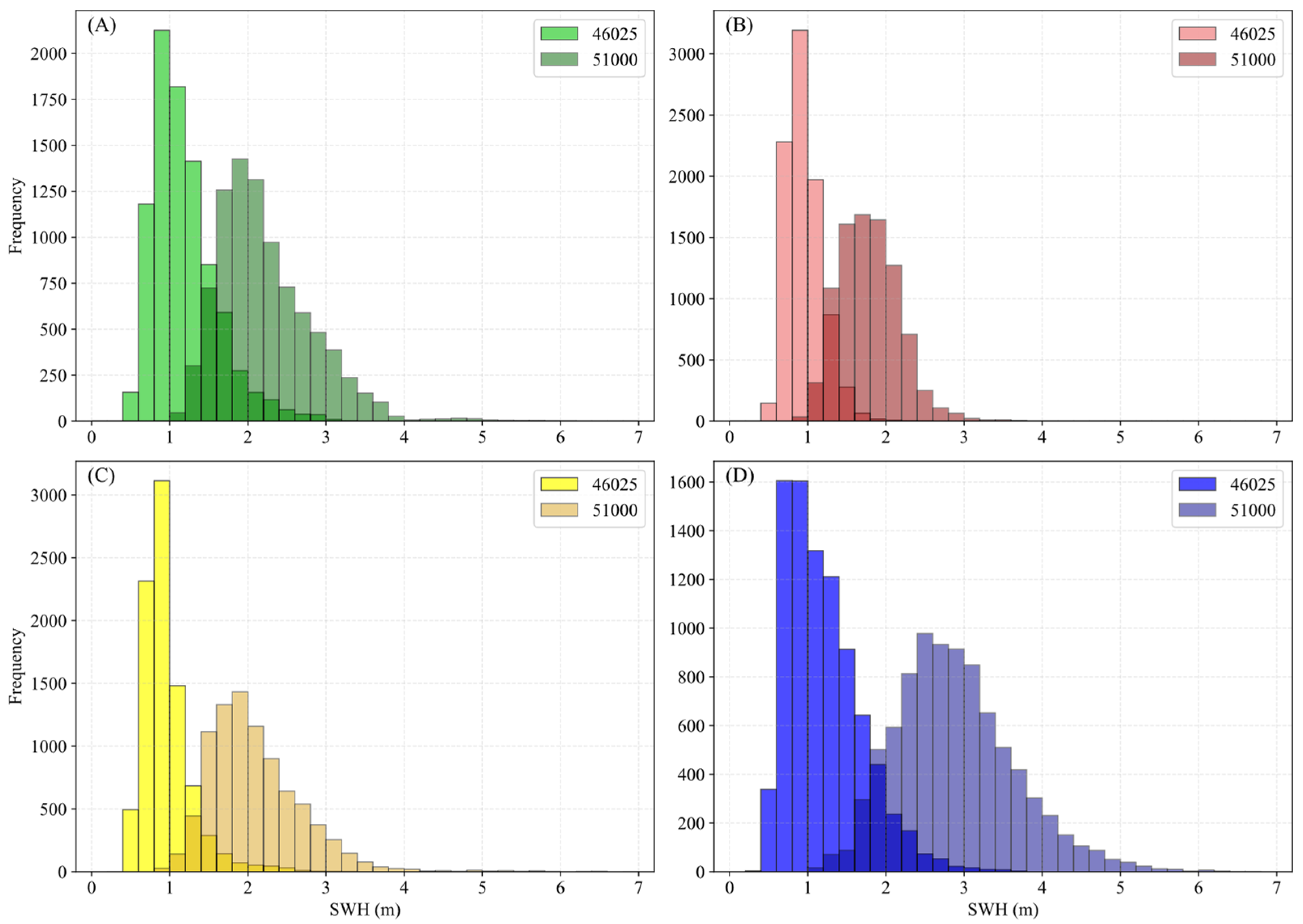
Statistical results (

Table 2. Statistical indicators of SWH data for the two stations.

Station	Average Value	Standard Deviation	Variance	Missing No.	Total No.
46025	1.075	0.391	0.153	783	35,064
51000	2.244	0.729	0.531	554	35,064
Station	Maximum Value	Minimum Value	First Quartile	Median	Third Quartile
46025	3.758	0.366	0.805	0.978	1.245
51000	7.291	0.864	1.725	2.083	2.634

) show that the mean SWH at Station 51000 is 2.24 m, which is significantly higher than that at Station 46025 (1.08 m). The maximum SWH at Station 51000 reaches 7.29 m, approximately twice the value recorded at Station 46025 (3.76 m). Station 51000 shows 247% greater SWH variance than Station 46025, confirming more pronounced wave fluctuations in open-ocean environments. Seasonally (Figure 2), SWH distributions at Station 46025 remain consistent across all seasons, predominantly concentrated within 0.60–1.40 m. Conversely, Station 51000 demonstrates distinct seasonal patterns: lower SWH in summer (June to August) and higher values in winter (December to February). Summer SWH rarely exceeds 2.40 m, while winter values typically range between 2.00 and 3.40 m. The variances of SWH for Stations 46025 and 51000 across spring, summer, autumn, and winter are 0.17, 0.05, 0.10, and 0.23 and 0.37, 0.15, 0.37, and 0.59, respectively. These values highlight the characteristic of larger SWH fluctuations in winter and smaller fluctuations in summer.

2.2. Cointegration Test

The Engel–Granger cointegration test is employed to identify variables exhibiting long-term stable relationships with SWH. The procedure consists of the following steps:

(1)

Perform Augmented Dickey–Fuller (ADF) unit root tests [46] on all variable time series to determine their order of integration. Only pairs of time series sharing the same integration order qualify for subsequent cointegration testing. At both stations, sea surface temperature is identified as $I\left(1\right)$, while the other seven variables are $I\left(0\right)$.

(2)

For time-series pairs with identical integration orders, construct an ordinary least squares (OLS) regression. Taking the SWH series $a$ and the $k$-th correlated variable series $c^k$(same integration order) as an example:

$$a={\alpha }_0+{\alpha }_1{c}^k+{\mu }^k$$

(2)

where ${\alpha }_0$ and ${\alpha }_1$ are OLS regression coefficients and ${\mu }^k$ denotes the residual series.

(3)

Conduct an ADF unit root test on the residual series ${\mu }^k$. If ${\mu }^k$ is stationary, a cointegration relationship exists between $a$ and $c^k$; otherwise, no cointegration relationship is present.

(4)

Repeat Steps 2 and 3 to establish cointegration relationships across all qualifying time-series pairs.

2.3. Granger Causality Test

The Granger causality test [47] is employed to further determine causal relationships between variables with long-term stability. The procedure comprises the following steps:

(1)

For variable pairs passing the cointegration test, we first posit the null hypothesis that no Granger causality exists between SWH series $a$ and the $k$-th variable series $c^k$.

(2)

Construct vector autoregression models for $a$ and $c^k$ using Equations (3) and (4), then compute regression coefficients and residuals:

$$r_t={\rho }_0+{\rho }_1{r}_{t-1}+ \cdots +{\rho }_m{r}_{t-m}+{\xi }_1{c}_1^k+ \cdots +{\xi }_m{c}_{t-m}^k+{\lambda }_t$$

(3)

$$c_t^k={\delta }_0+{\delta }_1{c}_{t-1}^k+\cdots +{\delta }_m{c}_{t-m}^k+{ϵ}_1{r}_1+\cdots +{ϵ}_m{r}_{t-m}+{\nu }_t$$

(4)

where $m$ denotes the lag order; $r_{t-i}$ and $c_{t-i}^k$ $(i=1,\cdots ,m)$ represent lagged values; ${\rho }_0$ and ${\delta }_0$ are intercept terms; ${\rho }_i$, ${\delta }_i$, ${\xi }_i$, ${ϵ}_i$ $\in i$ are coefficients; and ${\lambda }_t$, ${\nu }_t$ denote residuals.

(3)

An F-statistic test is performed on the residuals. If the F-statistic is significant (typically with p < 0.05), the null hypothesis is rejected, confirming Granger causality between $a$ and $c^k$. Otherwise, the null hypothesis fails to be rejected.

(4)

Iterate through all cointegrated variable pairs to identify those with stable causal relationships.

2.4. Shapley Additive Explanations

The Python library developed by the Su-In Lee laboratory and Microsoft Research [48] is employed to conduct interpretability analysis of our proposed C-mLSTM model. The Shapley additive explanations (SHAP) value [49,50] is calculated as follows:

$$SHAP\left(X_j\right)=\sum _{S\in N}{\displaystyle \frac{k!\left(p-k-1\right)!}{p!}}[f(S\cup \{j\}))-f(S)]$$

(5)

where $p$ denotes the total number of features, $N$ represents the complete set of features excluding $X_j$, $S$ is a feature set in $N$, $f\left(S\right)$ is the model prediction with features in $S$, and $f(S\cup \{j\left\}\right)$ is the model prediction with features in $S$ plus feature $X_j$. $SHAP\left(X_j\right)$ quantifies feature $X_j$’s contribution, computed as the average of the marginal contributions to the model’s prediction across all possible models formed by different feature combinations.

2.5. Twin Delayed Deep Deterministic Policy Gradient Agent Architecture

The twin delayed deep deterministic policy gradient (TD3) agent framework comprises three key components:

(1)

Optimization objective

The agent aims to minimize the mean squared error (MSE) of wave forecasting as the optimization objective, as shown in Equation (6):

$$MSE={\displaystyle \frac{1}{n}}\sum _{i=1}^n({\widehat{y}}_i-y_i{)}^2$$

(6)

where $n$ is the total number of forecast samples, ${\widehat{y}}_i$ is the predicted value for the $i$-th sample, and $y_i$ is the observed value for the $i$-th sample.

(2)

Temporal constraints

To ensure the stability and efficiency of the agent’s training process, the range of variation for the time-window length is bounded by the following formula:

$$0<T_{min}\le T_{current}\le T_{max}$$

(7)

where $T_{min}$ and $T_{max}$ are the minimum and maximum lengths of the time window, which are set to 7 and 50 in this paper, respectively. $T_{current}$ is the current time-window length, which changes based on the historical data and historical loss values.

(3)

Markov decision process condition design

(1)

Agent state space

The state space $\left(s_t\right)$ serves as the core basis for the agent’s perception of the environment. A reasonable design of the state provides the foundation for the agent to make optimal decisions. The state design is shown in Equation (8):

$$s_t=\left[l_{t-i},\dots ,l_{t-1},los{s}_{t-i},\dots ,los{s}_{t-1}\right]$$

(8)

where $l_{t-i}$ is the historical wave data from the $i$-th time step, with $l$ referring to the 8 variables listed in Table 1, and $los{s}_{t-i}$ is the forecasting error in the $i$-th forecast cycle of the wave forecasting system.

• (2)

  Agent action

During the execution of the TD3 agent’s actions, the agent interacts with the environment based on the current state and the output from the policy network. Given that the correlation between historical data and future predictions is inversely proportional to the time interval, this paper adopts a unilateral adjustment strategy. The agent’s action design only adjusts the left edge of the time window, while the right edge is updated dynamically through a rolling mechanism to receive the latest historical data. This design ensures the dynamic adjustment of the window while effectively retaining highly correlated historical information. The specific action magnitude design is as follows:

$$a_t=T_{max}·{\widehat{a}}_{t+1}$$

(9)

where ${\widehat{a}}_{t+1}$ is the action magnitude output by the agent, with a range of [−1, 1]. $T_{max}·{\widehat{a}}_{t+1}$ represents the change in the window length.

• (3)

  Agent reward function

This paper establishes a dynamic reward and penalty mechanism, as shown in Equation (10). When the window length, $T_{current}$, reaches the boundary constraints, $T_{min}$ or $T_{max}$, the agent receives a fixed negative penalty term, $\mathsf{\zeta }$, set to −0.1 in this paper, to guide the agent’s optimization within the feasible range. Otherwise, the agent is rewarded with the negative value of the forecasting error based on the adjusted window length.

$$r_t=\left\{\begin{array}{c}\zeta , T_{current}\ge T_{max} or T_{current}\le T_{min}\\ -los{s}_{T_{current}}, otherwise\end{array}\right.$$

(10)

where $los{s}_{T_{current}}=({\widehat{y}}_i-y_i{)}^2$ represents the forecast error in the current ($i$-th) prediction cycle and $N^{\prime }$ is the forecasting step size.

2.6. The Construction of the Model

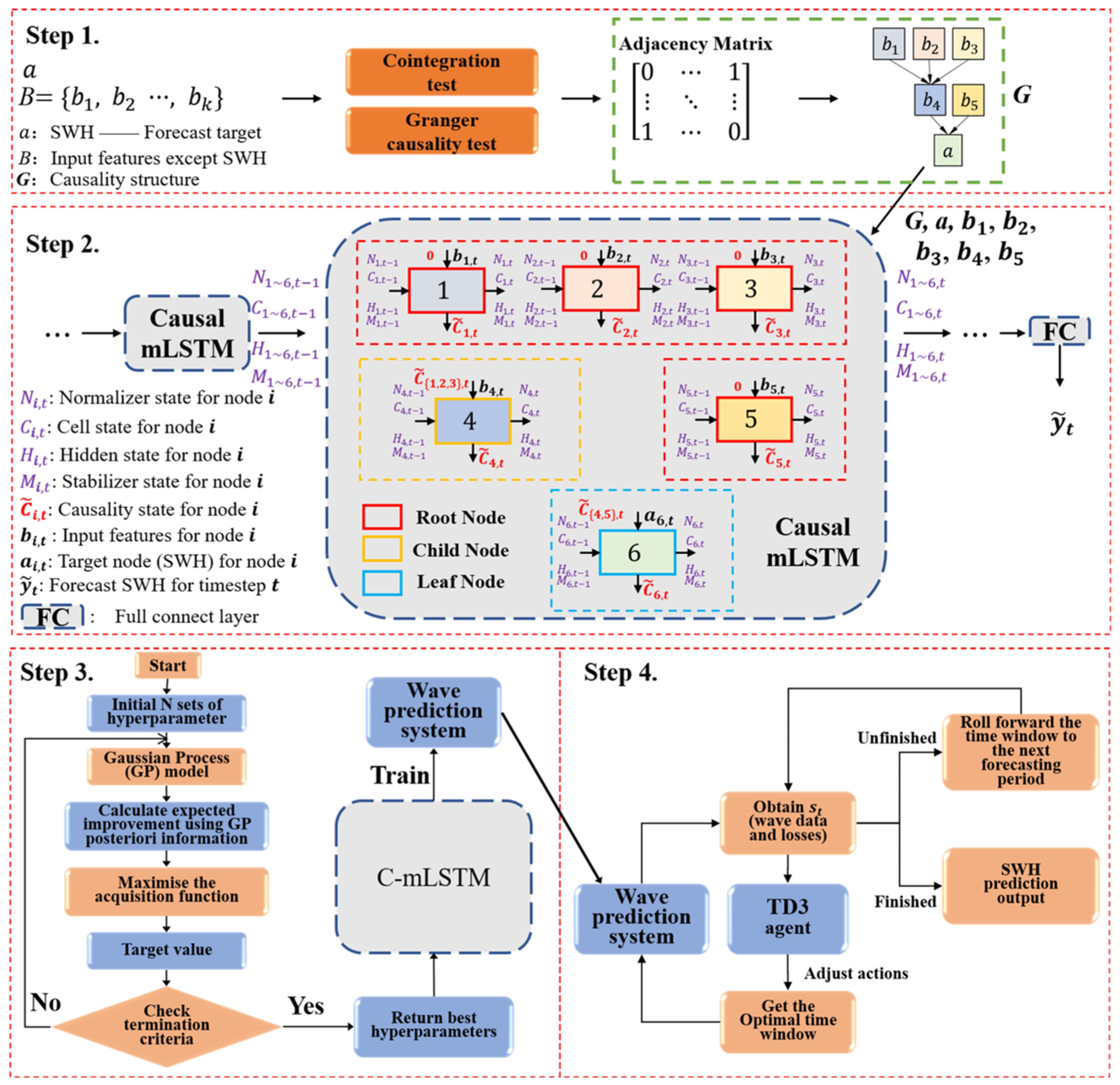
The C-mLSTM framework involves four primary steps from data processing to model construction, with its flowchart depicted in Figure 3.

2.6.1. Construction of the Causal Relationship Dataset

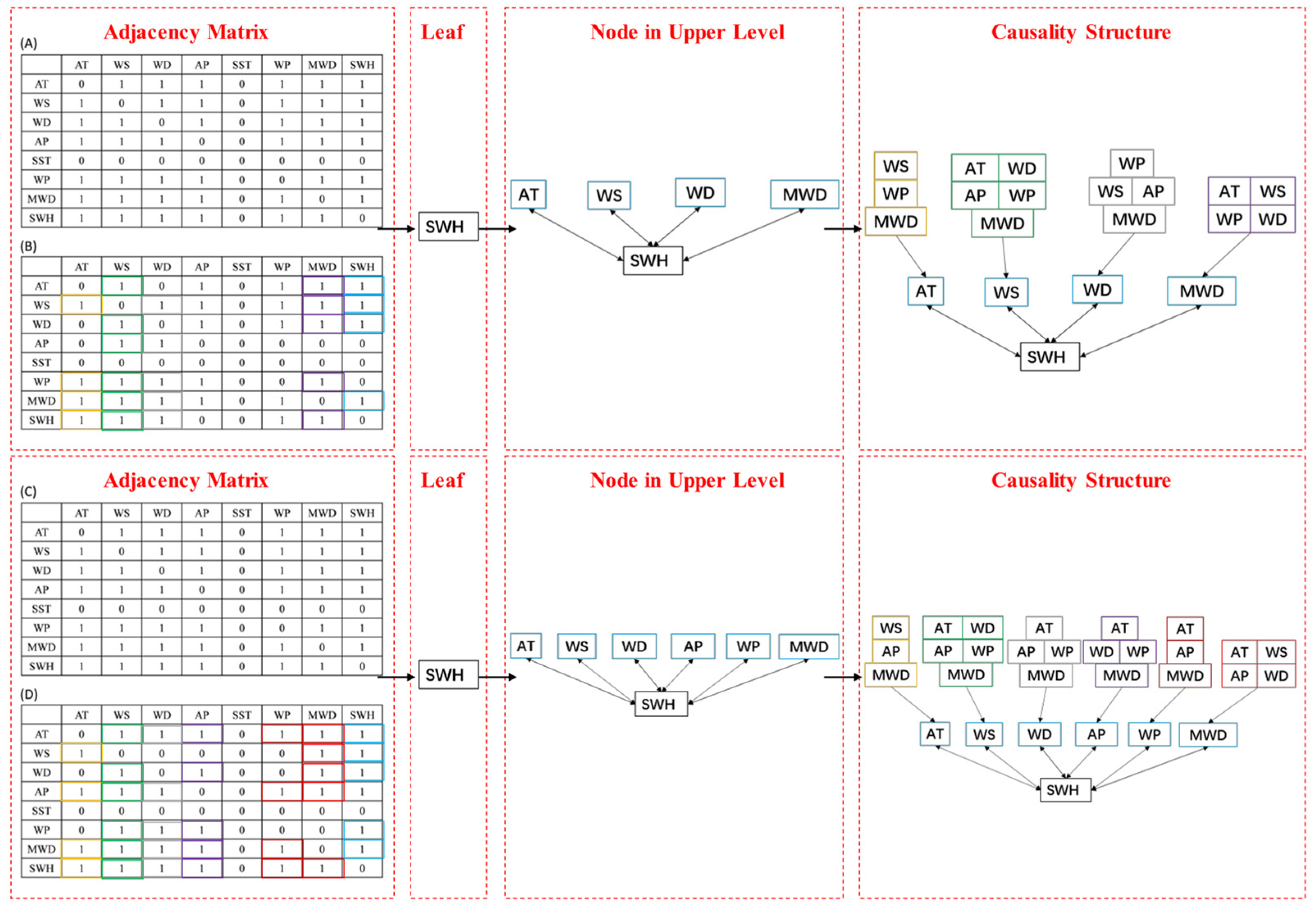
Step 1 constructs the causal relationship dataset (Figure 3). $a$ denotes the prediction target (SWH), $B$ represents the input variables from Table 1 excluding SWH, and $k$ indicates the $k$-th input feature. The adjacency matrix is denoted by $G$. Figure 4 illustrates the complete process of converting the adjacency matrix into the causal relationship dataset, corresponding to the green box in Step 1 of Figure 3. The procedure is detailed below:

(1)

Two-stage causal feature selection is performed on input features $B$ and target $a$. In phase 1, cointegration tests identify variable pairs with long-term stable relationships (Section 2.2). In phase 2, Granger causality tests (Section 2.3) further explore causal relationships among variables exhibiting long-term stability. This two-stage selection reveals long-term stable causal relationships.

(2)

Convert pairs of variables with long-term stable causal relationships into an adjacency matrix $(G$). For any two variables (e.g., $b_1$ and $b_4$), $G_{b_1,b_4}=1$ indicates that $b_1$ is a long-term causal driver of $b_4$ ($b_1$→$b_4$). $G_{b_1,b_4}=0$ indicates no long-term causal relationship. Figure 4A,B show cointegration and Granger test results for Station 51000; Figure 4C,D show results for Station 46025. Notably, Station 46025 (nearshore) has two additional variables (AP and WP) causally related to SWH compared to Station 51000 (open sea), likely due to coastal terrestrial influences.

(3)

Transform the adjacency matrix into the long-term causal relationship dataset (Figure 4). The conversion involves four steps (using Station 51000 as an example): First, set prediction target SWH as the leaf node. Additionally, assign SWH’s causal drivers (AT, WS, WD, and MWD, indicated by the blue boxes) as parent nodes of the leaf. What is more, for variables in the blue boxes, repeat the previous step to identify their causal drivers and assign them as parent nodes. Finally, starting from the root node, compile each variable’s index, parent count, and parent indices into the dataset.

2.6.2. The Construction of Causality-Structured Matrix Long Short-Term Memory

Step 2 in Figure 3 constructs the C-mLSTM. mLSTM was proposed by Beck et al. [51] with reference to bidirectional associative memory [52,53], enhancing memory capacity [54] compared to classical LSTM [55]. It extends the memory cell from scalar $C\in R$ to matrix $C\in R^{d\times d}$ and introduces an exponential activation function (replacing the sigmoid function) in the input gate, where $d$ is the hidden dimension within the mLSTM block [56]. To incorporate causal information into mLSTM, we introduce a new state for each node, $i$ (termed the causal state, denoted ${\tilde{\mathit{C}}}_i$), to constrain the mLSTM hidden state ($H_i$). Finally, the causal state (${\tilde{\mathit{C}}}_i$) of the leaf node (SWH) is fed into a fully connected layer for SWH prediction, as it contains both temporal dependency information and causal relationships.

Figure 5 shows the internal structure of a single node within the Causal mLSTM block. The green section is the mLSTM unit; the blue section is the causal inference unit proposed by Li et al. [40]. Taking node $i$ at timestep $t$ as an example, inputs include the following: input feature $X_{i,t}$, hidden state $H_{i,t-1}$, cell state $C_{i,t-1}$, normalizer state $N_{i,t-1}$, and additional state $M_{i,t-1}$ from the previous timestep, along with the set of causal states ${\tilde{C}}_{P_i,t}$ from parent nodes ($P_i$ denotes the set of indices for the parent nodes of node $i$). The Causal mLSTM block learns temporal dependencies by adopting the standard mLSTM computation [51] and captures causal relationships via Equations (11)–(16).

Causal regulation gate:

$${\gamma }_{i,t}=\sigma \left(W_{i,\gamma ,X}{X}_{i,t}+W_{i,\gamma ,H}{H}_{i,t-1}+b_{i,\gamma }\right)$$

(11)

Hidden regulation gate:

$${\delta }_{i,t}=\sigma \left(W_{i,\delta ,X}{X}_{i,t}+W_{i,\delta ,H}{H}_{i,t-1}+b_{i,\delta }\right)$$

(12)

Causal weight gate:

$${\alpha }_{P_i,t}=\sigma \left(W_{i,\alpha ,X}{X}_{i,t}+W_{i,\alpha ,H}{H}_{i,t-1}+b_{i,\alpha }\right)$$

(13)

Causal weight for node $j$:

$${\beta }_{j,t}={\alpha }_{j,t}\odot {\tilde{C}}_{j,t}$$

(14)

Parent causal weight:

$$L_{i,t}=\sum _{j\in P_i} {\beta }_{j,t}$$

(15)

Causal state:

$$\begin{array}{c}{\tilde{C}}_{i,t}={\gamma }_{i,t}\odot L_{i,t}+{\delta }_{i,t}\odot H_{i,t}\end{array}$$

(16)

where $W_{\ast }$ denotes weights; $b_{\ast }$ denotes biases; $\sigma$,$exp$, and $log$ denote sigmoid, exponential, and logarithmic functions; $\odot$ denotes element-wise multiplication; and $\sum$ denotes summation. Root nodes (nodes without parents, e.g.,$b_1$, $b_2$, $b_3$, and $b_5$, in Step 1 of Figure 3) have ${\tilde{C}}_{P_i,t}=0$.

2.6.3. Bayesian Optimization for Hyperparameter Tuning

Step 3 of model construction optimizes C-mLSTM hyperparameters using Bayesian optimization (BO). The BO [42,43,57] hyperparameter optimization process comprises six steps: (1) Initialize hyperparameter sets. Randomly sample N initial hyperparameter combinations within predefined search spaces. (2) Build a Gaussian Process (GP) regression model. (3) Calculate Expected Improvement (acquisition function) using posterior information from the GP model. (4) Optimize the acquisition function to select the next hyperparameter point. (5) Obtain the loss function through C-mLSTM model training. (6) Check termination criteria (maximum iterations reached). If satisfied, train final C-mLSTM with optimal hyperparameters; otherwise, repeat steps.

This study employs BO for automatic tuning of critical hyperparameters: batch size, learning rate, and number of hidden units. Batch size and hidden units are searched in discrete space: {8, 16, 32, 64, 128, 256, 512}, and the learning rate is optimized in a continuous interval: [10⁻⁵, 10⁻¹]. The process terminates at 50 iterations, with minimum validation MSE as the optimization criterion. When 50 iterations are reached, the combination yielding the lowest validation MSE is selected for the final model parameters. Detailed results for the BO of models are shown in

Table 3. Results for BO of models.

	Default Value	LSTM	mLSTM	C-mLSTM
Batch size	{8, 16, 32, 64, 128, 256, 512}	32	8	16
Hidden layer size	{8, 16, 32, 64, 128, 256, 512}	64	128	128
Learning rate	[10−5, 10−1]	0.0057578	0.0046483	0.0039066

.

2.6.4. Twin Delayed Deep Deterministic Policy Gradient for Dynamic Input Window Adjustment

Step 4 in Figure 3 is the process of dynamically adjusting the input window using the twin delayed deep deterministic policy gradient (TD3). This study employs the TD3 reinforcement learning algorithm to dynamically optimize the time window of the C-mLSTM model based on historical data and historical forecasting loss. By adaptively adjusting the time-window length, the method balances information retention and redundancy reduction to enhance forecasting accuracy. During the system initialization phase, initial parameters for both the wave forecasting model and the TD3 agent are loaded synchronously. Then, the agent makes decisions based on historical input data and the loss function values, dynamically adjusting the size of the time window. A reward mechanism guides optimal window selection to minimize prediction error. In each prediction cycle, the SWH forecasting model makes predictions based on the time window adjusted by the agent and provides the prediction results back to the agent for continuous optimization. After completing one prediction cycle, the time window is rolled forward to the next prediction cycle according to a predetermined step size, enabling real-time updates and optimization.

2.7. Model Training and Evaluation

The dataset was chronologically partitioned into training (60%), validation (20%), and test (20%) sets to prevent future data leakage [58]. Three model architectures (LSTM, mLSTM, and C-mLSTM) were developed using eight input variables from Table 1 to forecast SWH for 1, 3, 6, 12, and 24 h lead times. Station-specific models were independently established for reliability. It is noteworthy that only causality-structured models (e.g., C-mLSTM) necessitate the construction of causal relationship datasets. These datasets enhance model performance by capturing long-term stable causal dependencies among input features, and their construction processes vary according to the data characteristics of different stations.

Two optimization strategies were employed during the training process to prevent overfitting: (1) An early stopping mechanism: Training was halted if validation loss showed no improvement for 50 consecutive epochs. (2) Dynamic learning rate adjustment: The learning rate was reduced by a factor of 10 when validation loss plateaued for 10 consecutive epochs. Models were selected based on minimal validation MSE. The validation set also trained the TD3 agent for dynamic input window optimization. The configurations used in the experiment are shown in

Table 4. Experimental hardware and software configuration.

Component	Specification
Operating System	Microsoft Windows 10
CPU	Intel Core i5 13600K (14 cores, 20 threads)
GPU	NVIDIA GeForce RTX 4070 (12 GB)
Memory	64 G DDR5 (4800 MHz)
Software Stack	Python 3.9.18, torch 2.3.0+cu121, tensorflow-gpu 2.7.0

. The training time for an epoch of LSTM, mLSTM, and C-mLSTM was 15 s, 15 s, and 300 s, respectively, with a total of 200 training epochs, and adaptive moment estimation was used as the optimizer. It is worth noting that the C-mLSTM model converges significantly faster (60 epochs) than the other models (110 epochs).

The model performance was comprehensively evaluated using the following metrics: mean squared error (MSE), mean absolute error (MAE), root mean squared error (RMSE), coefficient of determination (R²), and mean absolute percentage error (MAPE). The formulas for these metrics are as follows:

$$MSE={\displaystyle \frac{1}{n}}\sum _{i=1}^n({\widehat{y}}_i-y_i{)}^2$$

(17)

$$MAE={\displaystyle \frac{1}{n}}\sum _{i=1}^n|{\widehat{y}}_i-y_i|$$

(18)

$$RMSE=\sqrt{{\displaystyle \frac{1}{n}}\sum _{i=1}^n{({\widehat{y}}_i-y_i)}^2}$$

(19)

$$R^2=1-{\displaystyle \frac{\sum _{i=1}^n{({\widehat{y}}_i-y_i)}^2}{\sum _{i=1}^n{(y_i-\overline{y})}^2}}$$

(20)

$$MAPE={\displaystyle \frac{100\%}{n}}\sum _{i=1}^n|{\displaystyle \frac{{\widehat{y}}_i-y_i}{y_i}}|$$

(21)

where $n$ is the total number of forecast samples, ${\widehat{y}}_i$ is the predicted value for the $i$-th sample, and $y_i$ is the true value for the $i$-th sample. $\overline{y}$ is the average value for $n$ samples.

3. Results

3.1. Ablation Experiment

To investigate performance variations of the LSTM, mLSTM, and C-mLSTM models before and after integrating the BO and TD3 algorithms,

Table 5. Evaluation metrics for models at Station 51000 for 12 h lead time.

	RMSE (m)	MAE (m)	R2	MAPE (%)
LSTM	0.3483	0.2361	0.7460	11.6126
mLSTM	0.3439	0.2303	0.7520	11.3353
C-mLSTM	0.3304	0.2244	0.7711	11.0577
TD3-LSTM	0.3475	0.2335	0.7471	11.4408
TD3- mLSTM	0.3435	0.2298	0.7527	11.3077
TD3-C-mLSTM	0.3283	0.2215	0.7741	10.8443
BO-LSTM	0.3232	0.2146	0.7811	10.2978
BO-mLSTM	0.3228	0.2172	0.7816	10.5462
BO-C-mLSTM	0.3163	0.2131	0.7902	10.1948
TD3-BO-LSTM	0.3219	0.2153	0.7828	10.3713
TD3-BO-mLSTM	0.3189	0.2125	0.7868	10.2509
TD3-BO-C-mLSTM	0.3150	0.2118	0.7920	10.1023

presents their 12 h forecasting metrics. Hyperparameters for baseline models (without BO) were standardized: 8 hidden units, a learning rate of 0.001, and a batch size of 512. C-mLSTM consistently outperformed LSTM and mLSTM across all metrics, both in baseline configurations and when enhanced with TD3 and BO optimization. This demonstrates the superiority of causal architecture over traditional non-causal structures.

Notably, in specific cases (e.g., BO-LSTM vs. TD3-BO-LSTM), while optimized TD3-BO-LSTM reduced RMSE and increased R², MAE and MAPE increased. This occurred because the model training, BO hyperparameter optimization, and TD3 window adjustment all used MSE (squared RMSE) as the loss function. Meanwhile, MSE’s squaring operation increases sensitivity to outliers, prioritizing large-error samples. Optimization may thus reduce major errors while slightly increasing minor errors, explaining the RMSE-MAE divergence.

3.1.1. Analysis of BO Algorithm

To evaluate the impact of BO on model performance, this study compares metrics between the baseline models (LSTM, mLSTM, and C-mLSTM) and their BO-optimized counterparts (Table 5). The results demonstrate consistent performance improvements of 2.48–11.32% for BO-LSTM, BO-mLSTM, and BO-C-mLSTM over their respective baselines. Notably, LSTM exhibits the most significant enhancement after BO integration; mLSTM shows moderate improvement; C-mLSTM achieved the smallest gain. This indicates that compared to LSTM and mLSTM, the C-mLSTM architecture exhibits lower sensitivity to hyperparameter tuning, with its performance being less affected by initial hyperparameter settings or variations. These results confirm the capability of BO to enhance predictive accuracy through hyperparameter optimization.

3.1.2. Analysis of TD3 for Input Window Adjustment

Compared to the BO-mLSTM model without the TD3 component, the TD3-BO-C-mLSTM achieved improvements of 1.21% (RMSE), 2.16% (MAE), 0.67% (R²), and 2.80% (MAPE) (Table 5). While LSTM, mLSTM, and C-mLSTM all showed performance gains after TD3 integration, the improvements were marginal.

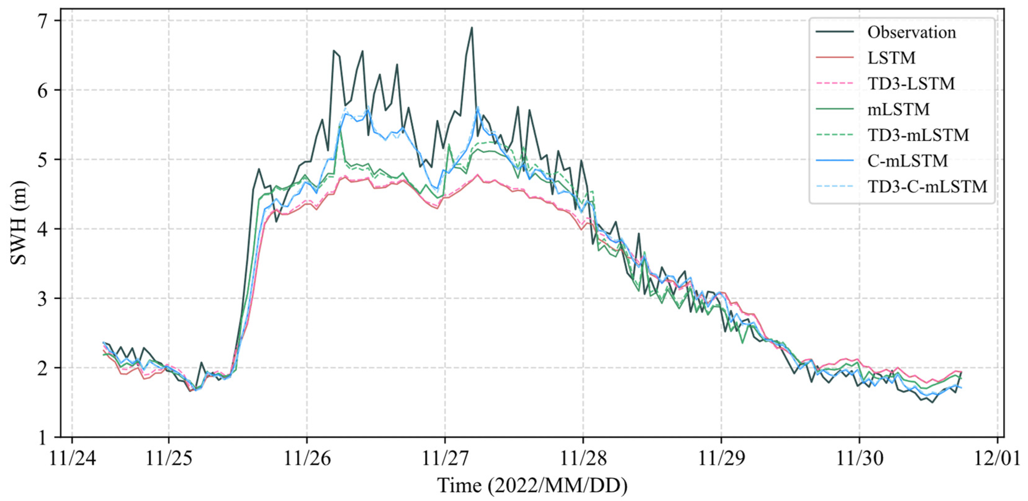
To further analyze how TD3 dynamically adjusts the input window length of the model, we plotted time-series diagrams comparing model predictions with observed values at Station 51000 (Figure 6). In Figure 6, the red, green, and blue lines represent prediction results from the LSTM, mLSTM, and C-mLSTM models, respectively, while solid and dashed lines indicate predictions before and after TD3 integration. When comparing solid and dashed lines of the same color (i.e., evaluating the same model with and without TD3), consistent overall trends can be observed between the two line types. However, during high-wave events (SWH > 4 m, significantly exceeding this station’s mean value of 2.244 m), predictions from models without TD3 (solid lines) were substantially lower than the observed values. In contrast, TD3-enhanced models (dashed lines) dynamically adjusted input window lengths based on historical SWH and loss function values, bringing predictions closer to true values and thereby reducing forecasting errors, while improving accuracy. When comparing curves of different colors (i.e., evaluating different models), the C-mLSTM model (blue) demonstrated optimal forecasting performance, showing particularly outstanding results during SWH > 4 m events. This indicates that C-mLSTM effectively utilizes causal relationships between variables revealed by the causal relationship dataset to deliver more accurate and reliable predictions. In summary, introducing the TD3 agent reduces discrepancies between predicted and true values to some extent, and among the three discussed models, C-mLSTM exhibits superior performance.

However, the TD3-C-mLSTM model still struggles to accurately forecast high SWH values. This is primarily due to the scarcity of high-value data, which leads to an imbalanced sample distribution and hinders the model’s ability to learn forecasting patterns in high-value regions. According to existing research [22], one potential solution is to train the model specifically using data from typhoon periods, thereby improving its capability to capture trends in high SWH ranges. However, this approach may simultaneously reduce forecasting accuracy for values within normal ranges.

3.2. Analysis of Seasonal Differences in Model Prediction Results

Figure 7 visually compares seasonal forecast performance across models for a 24 h lead time using radar charts. At Station 51000 (Figure 7A–D), all models demonstrate a consistent seasonal error pattern with a clear hierarchical order: winter errors are the highest, followed by autumn, then spring, and summer errors are the lowest. This occurs because models optimize for overall loss minimization, favoring predictions in high-density data regions. This corresponds to the distribution characteristics in Table 2, where the summer SWH shows small fluctuations, with data highly concentrated around the mean, while the winter SWH exhibits large fluctuations, with data primarily distributed above the third quartile percentile.

Station 46025 exhibits different characteristics, with spring and winter showing the largest and comparable errors, followed by autumn, while summer still maintains the smallest errors (Figure 7E–H). The causes of smaller errors during summer at this station are consistent with those at Station 51000, primarily attributed to the gentle fluctuations and concentrated distribution of SWH in this season. Although winter experiences significant wave variability, the statistical histogram in Figure 2 reveals relatively uniform SWH distribution near the peak value interval. Conversely, the spring histogram displays substantial data distribution fluctuations near the peak interval, indicating more complex multimodal features or transient mutation events during this season. This distribution difference likely constitutes an important factor contributing to the higher prediction difficulty and larger errors in spring.

Compared to the other models, the TD3-BO-C-mLSTM model achieves the smallest errors and largest R² values in most cases, particularly showing the most significant improvements during summer and winter at Station 51000 (Figure 7A–D). In conclusion, all models exhibit relatively inferior forecasting performance during winter, highlighting the need to improve their capability to learn extreme values. Compared to alternative models, the causality-enhanced C-mLSTM model proposed in this study demonstrates superior forecasting performance across all seasons. Its particularly pronounced advantage in winter forecasting at Station 51000 validates this model’s stronger generalization capability.

3.3. Analysis of Model Performance Across Lead Times

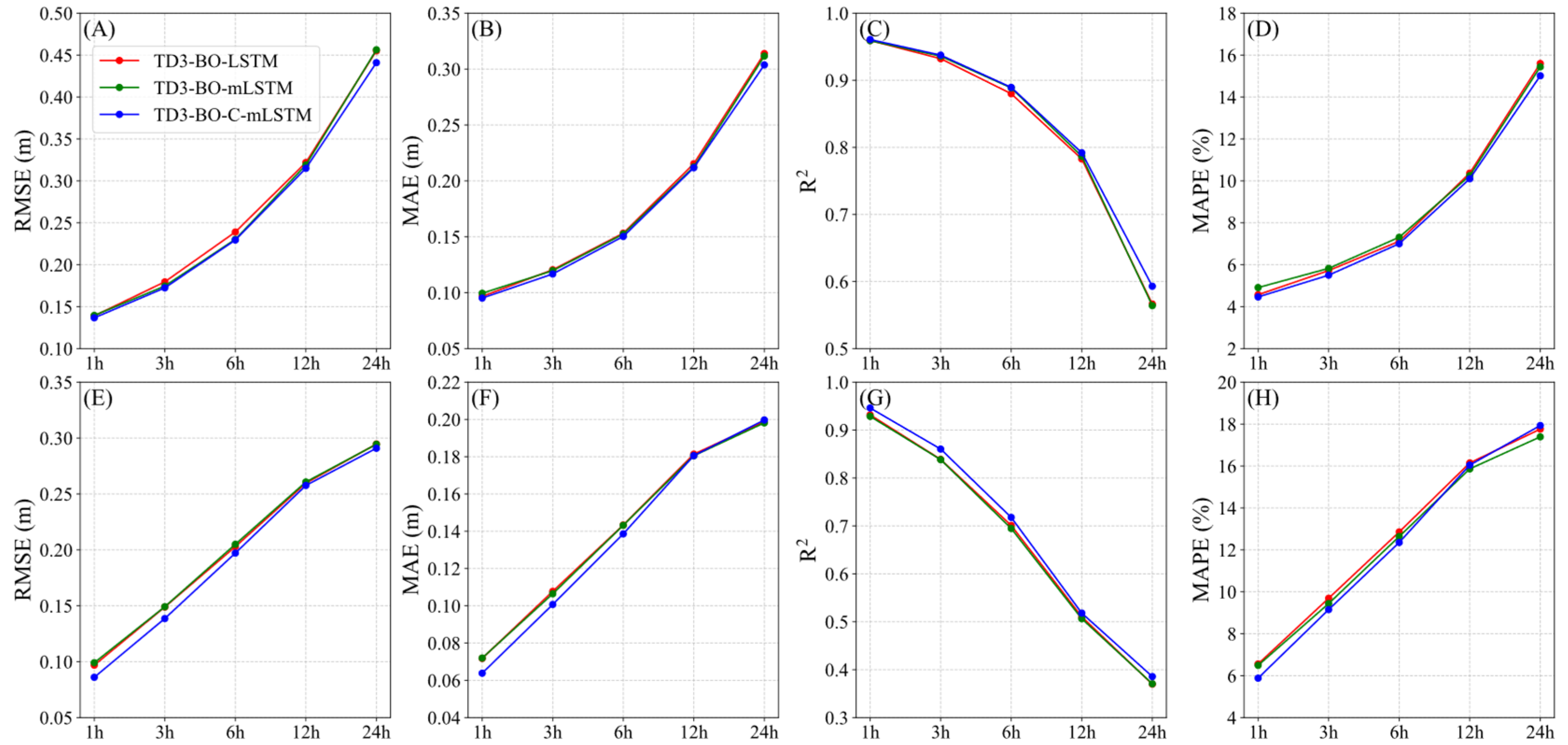
Figure 8 presents performance metrics of the TD3-BO-LSTM (red solid line), TD3-BO-mLSTM (green solid line), and TD3-BO-C-mLSTM (blue solid line) models across different lead times. Overall, predictive performance declines as the prediction step sizes increase. For the same lead-time predictions, Station 46025 demonstrates lower RMSE and MAE values than Station 51000. This discrepancy can be explained by the statistical characteristics of SWH in Table 2: Station 51000 exhibits a significantly greater SWH range and variance, indicating broader value fluctuations and consequently higher prediction difficulty.

The TD3-BO-C-mLSTM model generally achieves optimal performance for the same lead-time predictions, underperforming only marginally in MAE and MAPE at Station 46025’s 24 h horizon (Figure 8F,H). This phenomenon arises because MAPE is more sensitive to errors in observations with larger true values under the same absolute error magnitude, whereas MAE directly reflects the error level. For the 24 h lead time at Station 46025, TD3-BO-C-mLSTM prioritizes accurate prediction of larger SWH values, slightly compromising precision for smaller values. Other models focus more on overall average accuracy and smaller-value prediction. Given that ocean engineering prioritizes extreme SWH impacts, the performance characteristics of TD3-BO-C-mLSTM make it particularly suitable for such applications.

3.4. Model Predictive Capability for Rough Wave Conditions

This section further analyzes model performance for rough wave predictions (SWH ≥ 2.5 m) for a 24 h lead time (Figure 9). Compared to performance on the full test set (containing all SWH conditions), all models exhibit reduced accuracy when predicting rough wave events. This phenomenon occurs because SWH values exceeding 2.5 m exhibit lower occurrence frequency, leading to insufficient data volumes that impede models from capturing underlying patterns. Notably, the TD3-BO-C-mLSTM model outperforms all others, achieving the smallest RMSE and MAE values, which demonstrates its enhanced forecasting capability and robust performance under rough wave conditions.

Station 46025 shows substantially larger prediction errors than Station 51000, with its RMSE and MAE values being approximately double those of 51000. Detailed analysis reveals that while the 2.5 m threshold falls below the third quartile percentile at Station 51000, it approaches the maximum recorded value at Station 46025. Models typically prioritize predictions near mean or median values to minimize loss functions. However, Station 46025 contains only 36 extreme samples exceeding 2.5 m, significantly fewer than Station 51000’s 1354 such samples. This confirms that predicting extreme values remains a significant challenge for current models.

4. Discussion

4.1. Sensitivity Analysis of Causal Structure Depth

To investigate model performance across different hierarchical depths, this study conducted sensitivity experiments with three causal depth parameters (Depth = 2/3/4). Figure 10 presents boxplots of prediction errors from these configurations. In the visualization, the upper and lower black solid lines represent the maximum and minimum errors, respectively, while the red line indicates mean model errors. Blue scatter points depict error distributions between predictions and true values, and the boxes span the interquartile ranges (from the first quartile to the third quartile percentiles) of the errors. Results show that the Depth 2 configuration produces a slightly higher RMSE value of 0.1361 m compared to the Depth 3 (0.1347 m) and Depth 4 (0.1338 m) configurations. Furthermore, the error range (maximum–minimum error) for Depths 2, 3, and 4 measures 2.69 m, 2.48 m, and 2.48 m, respectively, indicating that Depth 2 exhibits greater error dispersion, while Depths 3 and 4 show nearly identical dispersion. Notably, per-epoch computation times were 150 s, 300 s, and 10,898 s for Depths 2, 3, and 4, respectively. Balancing prediction accuracy against computational efficiency, this study selected the Depth 3 configuration for final model training.

4.2. Shapley Additive Explanations Analysis

SHAP (Shapley additive explanations) analysis was conducted on the input features of the BO-C-mLSTM model. Figure 11A–D illustrate the impacts of input features on SWH forecasts for 1, 3, 12, and 24 h lead times, respectively. In these visualizations, SHAP absolute values quantify feature contribution magnitudes—larger absolute values indicate stronger influence (bar heights reflect values above the x-axis, while dot positions show values below).

Key findings reveal that historical SWH dominates SWH forecasting, followed by WS and WP, while SST and AP exhibit minimal contributions. As the prediction step sizes increase, the contribution of SWH decreases sharply—from 93% at the 1 h lead time to 40% at the 24 h lead time—while the contributions of WS and WP increase from 4% to 22% and from 2% to 21%, respectively. This demonstrates that while historical SWH governs for the 1 h lead time, WS and WP become increasingly significant for the 24 h lead time. Consistently, Figure 11A shows SWH dots possessing substantially larger SHAP absolute values than other features, but this dominance diminishes as the prediction step size increases, with WS, WP, and WD gaining influence, which aligns with the trends in the bar chart. Furthermore, Figure 11D indicates positive correlations between future SWH and historical SWH, WS, and WP, but a negative correlation with AT.

While the high SHAP values for SWH and WS in Figure 11D align with the causal graph in Figure 4A,B, variables such as AT, WD, and MWD—identified as causal drivers—show low SHAP contributions. This discrepancy arises because the causal graph reflects interventional relationships, whereas SHAP measures conditional predictive importance within the specific model context. In practice, effects from AT, WD, and MWD may be indirectly captured by correlated features, reducing their marginal contribution in the C-mLSTM predictions. Thus, the model refines the causal prior by emphasizing features with stronger predictive utility under specific lead times and regimes, rather than treating all causal links as equally relevant for forecasting.

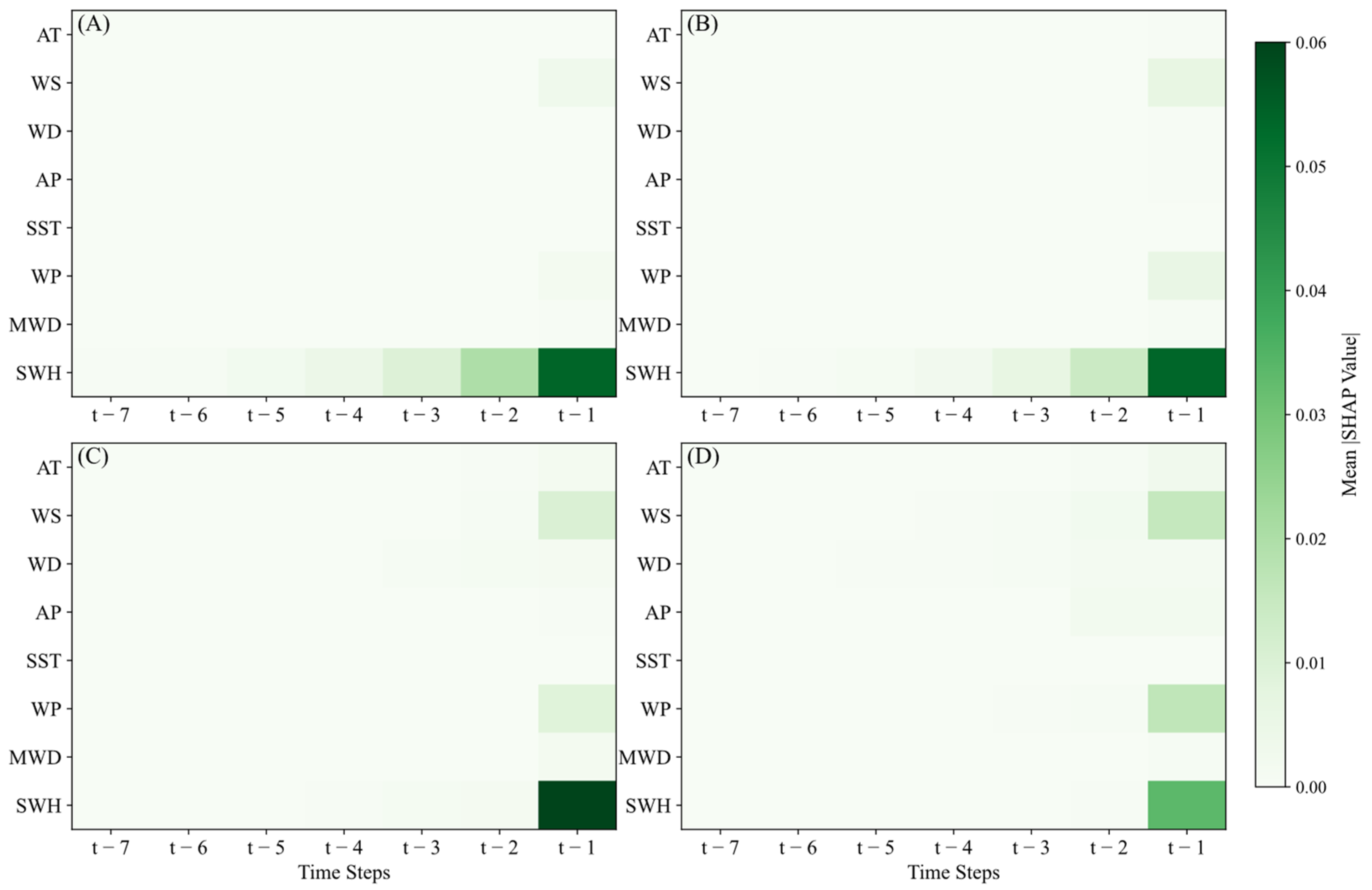
To investigate temporal dependencies, we performed time-step-specific SHAP analysis (Figure 12). The primary contributors to the 1 h ahead SWH forecast are SWH values from time steps t-5 to t-1 and WS/WP values at t-1, with the SWH from t-3 to t-1 playing a pivotal role. Contributions from other time steps are negligible, as shown in Figure 12A. With the increase in forecast lead time, the contribution of SWH from time steps t-5 to t-2 gradually decreases, while the contributions from AT, WS, WD, AP, and WP at time steps t-2 and t-1 gradually increase. The contribution of SST remains close to zero, which is consistent with the results of the two-stage causal feature analysis in Section 2.6.1 (Figure 4A).

In conclusion, for SWH forecasting, the features from the past five time steps account for 99% of the contribution and inputting too many time steps leads to data redundancy. For forecasts within 1 h, only the SWH feature plays a significant role, while for 24 h forecasts, the SST and MWD features can be disregarded.

4.3. Advantages and Limitations of C-mLSTM

LSTM, mLSTM, and C-mLSTM models are evaluated for SWH forecasting, with the causality-enhanced C-mLSTM architecture demonstrating superior performance. The model’s key strengths and constraints are as follows:

Advantages:

(1)

Inheriting the strength of mLSTM in capturing temporal patterns, C-mLSTM delivers exceptional performance for SWH time-series forecasting.

(2)

Its two-stage causal feature screening (cointegration and Granger causality tests) enables learning stable long-term causal relationships among variables, enhancing both predictive accuracy and interpretability.

(3)

In terms of model structure, the C-mLSTM incorporates a dedicated causal inference unit that generates causal states for each variable, enabling the model to align predictions with the causal drivers of the current nodes, thereby adjusting the output of the predictions.

(4)

In terms of prediction results, the C-mLSTM model outperforms the LSTM and mLSTM models, which do not incorporate causal structures, under both normal and rough wave conditions.

Limitations:

(5)

While the causal screening methodology fully utilizes variables in Table 1 (except SST), Granger causality tests possess inherent limitations in capturing nonlinear relationships [59].

(6)

Despite its superior predictive capability, C-mLSTM requires longer training times (300 s per epoch) compared to LSTM/mLSTM (15 s per epoch), potentially limiting time-sensitive applications.

(7)

Despite the superior performance of C-mLSTM, its predictions for high SWH values remain biased, primarily due to the scarcity of high-value samples in the training data.

5. Conclusions

This study proposes a novel C-mLSTM model for SWH forecasting, with key findings derived from interpretable SHAP analysis:

(1)

The two-stage causal feature selection (cointegration and Granger causality tests) constructs causal relationship datasets. Embedding these identified causal dependencies into the mLSTM framework enhances predictive performance and interpretability, demonstrating particular efficacy for time-series forecasting with complex causal structures.

(2)

In terms of model optimization, we incorporated the BO algorithm and the TD3 algorithm. BO improves average SWH prediction accuracy by 16.48% through hyperparameter tuning for all models (LSTM, mLSTM, and C-mLSTM). TD3 dynamically adjusts input window length based on historical data and historical loss values, yielding a further 2.35% accuracy gain. Combined implementation delivers 16.85% overall performance improvement.

(3)

Compared to conventional LSTM and mLSTM, C-mLSTM achieves superior performance for 1, 3, 6, 12, and 24 h lead times under both normal and rough wave conditions (SWH > 2.5 m). Its leading accuracy across seasons, multiple lead times, and extreme events confirms its enhanced robustness and generalization capability.

(4)

Finally, through SHAP analysis, it was found that in 1 h SWH forecasts, the contributions of SWH, WS, and WP features are dominant. In 24 h forecasts, historical SWH remains the primary driver, while WS and WP gain significance; only SST and MWD exhibit negligible impacts.

The validated efficacy of C-mLSTM motivates further development of causal–spatiotemporal coupled models for intelligent wave forecasting. Future research will extend this framework to two-dimensional wave prediction, advancing decision-support capabilities for marine hazard early-warning systems and ocean engineering.

References

1. Dinwoodie, I.; Catterson, V.M.; McMillan, D. Wave Height Forecasting to Improve Off-Shore Access and Maintenance Scheduling. In Proceedings of the 2013 IEEE Power & Energy Society General Meeting, Vancouver, BC, USA, 21–25 July 2013; pp. 1–5. [Google Scholar]
2. Vanem, E. Joint Statistical Models for Significant Wave Height and Wave Period in a Changing Climate. Mar. Struct. 2016, 49, 180–205. [Google Scholar] [CrossRef]
3. Taylor, J.W.; Jeon, J. Probabilistic Forecasting of Wave Height for Offshore Wind Turbine Maintenance. Eur. J. Oper. Res. 2018, 267, 877–890. [Google Scholar] [CrossRef]
4. Guillou, N.; Lavidas, G.; Chapalain, G. Wave Energy Resource Assessment for Exploitation—A Review. J. Mar. Sci. Eng. 2020, 8, 705. [Google Scholar] [CrossRef]
5. Caires, S.; Sterl, A. 100-Year Return Value Estimates for Ocean Wind Speed and Significant Wave Height from the ERA-40 Data. J. Clim. 2005, 18, 1032–1048. [Google Scholar] [CrossRef]
6. Chen, C.; Shiotani, S.; Sasa, K. Numerical Ship Navigation Based on Weather and Ocean Simulation. Ocean Eng. 2013, 69, 44–53. [Google Scholar] [CrossRef]
7. Chen, C.; Sasa, K.; Prpić-Oršić, J.; Mizojiri, T. Statistical Analysis of Waves’ Effects on Ship Navigation Using High-Resolution Numerical Wave Simulation and Shipboard Measurements. Ocean Eng. 2021, 229, 108757. [Google Scholar] [CrossRef]
8. Fazeres-Ferradosa, T.; Taveira-Pinto, F.; Vanem, E.; Reis, M.T.; Neves, L.D. Asymmetric Copula–Based Distribution Models for Met-Ocean Data in Offshore Wind Engineering Applications. Wind Eng. 2018, 42, 304–334. [Google Scholar] [CrossRef]
9. Fazeres-Ferradosa, T.; Welzel, M.; Schendel, A.; Baelus, L.; Santos, P.R.; Pinto, F.T. Extended Characterization of Damage in Rubble Mound Scour Protections. Coast. Eng. 2020, 158, 103671. [Google Scholar] [CrossRef]
10. Ardhuin, F.; Stopa, J.E.; Chapron, B.; Collard, F.; Husson, R.; Jensen, R.E.; Johannessen, J.; Mouche, A.; Passaro, M.; Quartly, G.D.; et al. Observing Sea States. Front. Mar. Sci. 2019, 6, 124. [Google Scholar] [CrossRef]
11. Han, Y.; Tang, J.; Jia, H.; Dong, C.; Zhao, R. A Significant Wave Height Prediction Method Based on Improved Temporal Convolutional Network and Attention Mechanism. Electronics 2024, 13, 4879. [Google Scholar] [CrossRef]
12. Liu, Y.; Lu, W.; Wang, D.; Lai, Z.; Ying, C.; Li, X.; Han, Y.; Wang, Z.; Dong, C. Spatiotemporal Wave Forecast with Transformer-Based Network: A Case Study for the Northwestern Pacific Ocean. Ocean Model. 2024, 188, 102323. [Google Scholar] [CrossRef]
13. Wang, X.; Jiang, H. Physics-Guided Deep Learning for Skillful Wind-Wave Modeling. Sci. Adv. 2024, 10, eadr3559. [Google Scholar] [CrossRef]
14. Group, T.W. The WAM Model—A Third Generation Ocean Wave Prediction Model. J. Phys. Oceanogr. 1988, 18, 1775–1810. [Google Scholar] [CrossRef]
15. Yuan, Y.; Hua, F.; Pan, Z.; Sun, L. LAGFD-WAM Numerical Wave Model. I: Basic Physical Model. Acta Oceanol. Sin. 1991, 10, 483–488. [Google Scholar]
16. Yuan, Y.; Hua, F.; Pan, Z.; Sun, L. LAGFD-WAM Numerical Wave Model. II: Characteristics Inlaid Scheme and Its Application. Acta Oceanol. Sin. 1992, 11, 13–23. [Google Scholar]
17. Booij, N.; Ris, R.C.; Holthuijsen, L.H. A Third-Generation Wave Model for Coastal Regions: 1. Model Description and Validation. J. Geophys. Res. Ocean. 1999, 104, 7649–7666. [Google Scholar] [CrossRef]
18. Tolman, H.L. User Manual and System Documentation of WAVEWATCH III ™ Version 3.14. Technical Note. 2019. Available online: https://polar.ncep.noaa.gov/mmab/papers/tn276/MMAB_276.pdf (accessed on 25 September 2025).
19. Hasselmann, S.; Hasselmann, K.; Allender, J.H.; Barnett, T.P. Computations and Parameterizations of the Nonlinear Energy Transfer in a Gravity-Wave Specturm. Part II: Parameterizations of the Nonlinear Energy Transfer for Application in Wave Models. J. Phys. Oceanogr. 1985, 15, 1378–1391. [Google Scholar] [CrossRef]
20. Tolman, H.L. Alleviating the Garden Sprinkler Effect in Wind Wave Models. Ocean Model. 2002, 4, 269–289. [Google Scholar] [CrossRef]
21. Zhou, S.; Wang, J.; Cao, Y.; Bethel, B.J.; Xie, W.; Xu, G.; Sun, W.; Yu, Y.; Zhang, H.; Dong, C. Improving the Accuracy of Global ECMWF Wave Height Forecasts with Machine Learning. Ocean Model. 2024, 192, 102450. [Google Scholar] [CrossRef]
22. Zhou, S.; Xie, W.; Lu, Y.; Wang, Y.; Zhou, Y.; Hui, N.; Dong, C. ConvLSTM-Based Wave Forecasts in the South and East China Seas. Front. Mar. Sci. 2021, 8, 680079. [Google Scholar] [CrossRef]
23. Guo, J.; Yan, Z.; Shi, B.; Sato, Y. A Slow Failure Particle Swarm Optimization Long Short-Term Memory for Significant Wave Height Prediction. J. Mar. Sci. Eng. 2024, 12, 1359. [Google Scholar] [CrossRef]
24. Shi, J.; Su, T.; Li, X.; Wang, F.; Cui, J.; Liu, Z.; Wang, J. A Machine-Learning Approach Based on Attention Mechanism for Significant Wave Height Forecasting. J. Mar. Sci. Eng. 2023, 11, 1821. [Google Scholar] [CrossRef]
25. Ouyang, Z.; Gao, Y.; Zhang, X.; Wu, X.; Zhang, D. Significant Wave Height Forecasting Based on EMD-TimesNet Networks. J. Mar. Sci. Eng. 2024, 12, 536. [Google Scholar] [CrossRef]
26. Fan, S.; Xiao, N.; Dong, S. A Novel Model to Predict Significant Wave Height Based on Long Short-Term Memory Network. Ocean Eng. 2020, 205, 107298. [Google Scholar] [CrossRef]
27. Wang, L.; Deng, X.; Ge, P.; Dong, C.; Bethel, B.; Yang, L.; Xia, J. CNN-BiLSTM-Attention Model in Forecasting Wave Height over South-East China Seas. Comput. Mater. Contin. 2022, 73, 2151–2168. [Google Scholar] [CrossRef]
28. Zacarias, H.; Marques, J.A.L.; Felizardo, V.; Pourvahab, M.; Garcia, N.M. ECG Forecasting System Based on Long Short-Term Memory. Bioengineering 2024, 11, 89. [Google Scholar] [CrossRef] [PubMed]
29. Chen, C.-H.; Lin, Y.-L.; Pai, P.-F. Forecasting Flower Prices by Long Short-Term Memory Model with Optuna. Electronics 2024, 13, 3646. [Google Scholar] [CrossRef]
30. Shi, N.; Xu, J.; Wurster, S.W.; Guo, H.; Woodring, J.; Van Roekel, L.P.; Shen, H.-W. GNN-Surrogate: A Hierarchical and Adaptive Graph Neural Network for Parameter Space Exploration of Unstructured-Mesh Ocean Simulations. IEEE Trans. Vis. Comput. Graph. 2022, 28, 2301–2313. [Google Scholar] [CrossRef]
31. Lei, L.; Tang, T.; Gang, Y.; Jing, G. Hierarchical Neural Network-Based Hydrological Perception Model for Underwater Glider. Ocean Eng. 2022, 260, 112101. [Google Scholar] [CrossRef]
32. Yang, H.; Li, W.; Hou, S.; Guan, J.; Zhou, S. HiGRN: A Hierarchical Graph Recurrent Network for Global Sea Surface Temperature Prediction. ACM Trans. Intell. Syst. Technol. 2023, 14, 73. [Google Scholar] [CrossRef]
33. Zhang, Y.; Feng, M.; Zhang, W.; Wang, H.; Wang, P. A Gaussian Process Regression-Based Sea Surface Temperature Interpolation Algorithm. J. Ocean. Limnol. 2021, 39, 1211–1221. [Google Scholar] [CrossRef]
34. Rychlik, I.; Johannesson, P.; Leadbetter, M.R. Modelling and Statistical Analysis of Ocean-Wave Data Using Transformed Gaussian Processes. Mar. Struct. 1997, 10, 13–47. [Google Scholar] [CrossRef]
35. Vinokić, L.; Dotlić, M.; Prodanović, V.; Kolaković, S.; Simonovic, S.P.; Stojković, M. Effectiveness of Three Machine Learning Models for Prediction of Daily Streamflow and Uncertainty Assessment. Water Res. X 2025, 27, 100297. [Google Scholar] [CrossRef]
36. Xie, W.; Xu, G.; Zhang, H.; Dong, C. Developing a Deep Learning-Based Storm Surge Forecasting Model. Ocean Model. 2023, 182, 102179. [Google Scholar] [CrossRef]
37. Musinguzi, A.; Akbar, M.K.; Fleming, J.G.; Hargrove, S.K. Understanding Hurricane Storm Surge Generation and Propagation Using a Forecasting Model, Forecast Advisories and Best Track in a Wind Model, and Observed Data—Case Study Hurricane Rita. J. Mar. Sci. Eng. 2019, 7, 77. [Google Scholar] [CrossRef]
38. Zhang, Z.; Qin, H.; Liu, Y.; Wang, Y.; Yao, L.; Li, Q.; Li, J.; Pei, S. Long Short-Term Memory Network Based on Neighborhood Gates for Processing Complex Causality in Wind Speed Prediction. Energy Convers. Manag. 2019, 192, 37–51. [Google Scholar] [CrossRef]
39. Dong, C.; Xu, G.; Han, G.; Bethel, B.J.; Xie, W.; Zhou, S. Recent Developments in Artificial Intelligence in Oceanography. Ocean-Land-Atmos. Res. 2022, 2022, 9870950. [Google Scholar] [CrossRef]
40. Li, L.; Dai, Y.; Shangguan, W.; Wei, Z.; Wei, N.; Li, Q. Causality-Structured Deep Learning for Soil Moisture Predictions. J. Hydrometeorol. 2022, 23, 1315–1331. [Google Scholar] [CrossRef]
41. Mockus, J.; Tiesis, V.; Zilinskas, A. The Application of Bayesian Methods for Seeking the Extremum. Towards Glob. Optim. 1978, 2, 117–129. [Google Scholar] [CrossRef]
42. Snoek, J.; Larochelle, H.; Adams, R.P. Practical Bayesian Optimization of Machine Learning Algorithms. In Advances in Neural Information Processing Systems; Curran Associates, Inc.: Red Hook, NY, USA, 2012; Volume 25. [Google Scholar]
43. Shahriari, B.; Swersky, K.; Wang, Z.; Adams, R.P.; de Freitas, N. Taking the Human Out of the Loop: A Review of Bayesian Optimization. Proc. IEEE 2016, 104, 148–175. [Google Scholar] [CrossRef]
44. Han, Y.; Zhao, R.; Wu, F.; Yan, J.; Dong, C. A Two Channel Optimized SWH Deep Learning Forecast Model Coupled with Dimensionality Reduction Scheme and Attention Mechanism. Ocean Eng. 2025, 330, 121217. [Google Scholar] [CrossRef]
45. Fujimoto, S.; Hoof, H.; Meger, D. Addressing Function Approximation Error in Actor-Critic Methods. In Proceedings of the 35th International Conference on Machine Learning; PMLR, Stockholm, Sweden, 10–15 July 2018; Volume 80, pp. 1587–1596. [Google Scholar]
46. Williams, J.T. What Goes Around Comes Around: Unit Root Tests and Cointegration. Political Anal. 1992, 4, 229–235. [Google Scholar] [CrossRef]
47. Granger, C.W.J. Investigating Causal Relations by Econometric Models and Cross-Spectral Methods. Econometrica 1969, 37, 424–438. [Google Scholar] [CrossRef]
48. Lundberg, S.M.; Lee, S.-I. A Unified Approach to Interpreting Model Predictions. In Proceedings of the 31st International Conference on Neural Information Processing Systems, Long Beach, CA, USA, 4–9 December 2017; Curran Associates Inc.: Red Hook, NY, USA, 2017; Volume 10, pp. 4768–4777. [Google Scholar]
49. Shapley, L.S. A Value for N-Person Games; RAND Corporation: Santa Monica, CA, USA, 1952. [Google Scholar]
50. Wu, T.; Xu, L.; Lv, Y.; Cai, R.; Pan, Z.; Zhang, X.; Zhang, X.; Chen, N. Integrating Causal Inference with ConvLSTM Networks for Spatiotemporal Forecasting of Root Zone Soil Moisture. J. Hydrol. 2025, 659, 133246. [Google Scholar] [CrossRef]
51. Beck, M.; Pöppel, K.; Spanring, M.; Auer, A.; Prudnikova, O.; Kopp, M.; Klambauer, G.; Brandstetter, J.; Hochreiter, S. xLSTM: Extended Long Short-Term Memory. Adv. Neural Inf. Process. Syst. 2024, 37, 107547–107603. [Google Scholar]
52. Anderson, J.A. A Simple Neural Network Generating an Interactive Memory. Math. Biosci. 1972, 14, 197–220. [Google Scholar] [CrossRef]
53. Anderson, J.A.; Silverstein, J.W.; Ritz, S.A.; Jones, R.S. Distinctive Features, Categorical Perception, and Probability Learning: Some Applications of a Neural Model. Psychol. Rev. 1977, 84, 413–451. [Google Scholar] [CrossRef]
54. Kohonen, T. Correlation Matrix Memories. IEEE Trans. Comput. 1972, C–21, 353–359. [Google Scholar] [CrossRef]
55. Hochreiter, S.; Schmidhuber, J. Long Short-Term Memory. Neural Comput. 1997, 9, 1735–1780. [Google Scholar] [CrossRef] [PubMed]
56. Alkin, B.; Beck, M.; Pöppel, K.; Hochreiter, S.; Brandstetter, J. Vision-LSTM: xLSTM as Generic Vision Backbone. In Proceedings of the Thirteenth International Conference on Learning Representations, Singapore, 24–28 April 2025. [Google Scholar]
57. Bergstra, J.; Bardenet, R.; Bengio, Y.; Kégl, B. Algorithms for Hyper-Parameter Optimization. In Proceedings of the 25th International Conference on Neural Information Processing Systems, Granada, Spain, 12–15 December 2011; pp. 2546–2554. [Google Scholar] [CrossRef]
58. Shi, X.; Chen, Z.; Wang, H.; Yeung, D.-Y.; Wong, W.; Woo, W. Convolutional LSTM Network: A Machine Learning Approach for Precipitation Nowcasting. In Proceedings of the 29th International Conference on Neural Information Processing Systems, Montreal, QC, Canada, 7–12 December 2015. [Google Scholar]
59. Baek, K.G.; Brock, W.A. A Nonparametric Test for Independence of A Multivariate Time Series. Stat. Sin. 1992, 2, 137–156. [Google Scholar]
Figure 1. Locations of NDBC buoys at Stations 51000 and 46025. Station 51000 (depth: 4762 m) is denoted by the red rectangle (23.528° N, 153.792° W), while Station 46025 (depth: 890 m) is indicated by the blue rectangle (33.755° N, 119.045° W). Water depth is represented by color shading.
Jmse 13 01872 g001
Figure 2. Seasonal histograms for SWH at Stations 46025 and 51000. Panels (AD) represent spring (March to May), summer (June to August), autumn (September to November), and winter (December to February), respectively. Histograms in vibrant hues correspond to Station 46025, while muted tones denote Station 51000.
Jmse 13 01872 g002
Figure 3. Flowchart of the TD3-BO-C-mLSTM model construction. Step 1: Constructing two-stage causal feature relationships. Step 2: Building the internal architecture of C-mLSTM. Step 3: Applying the Bayesian optimization (BO) algorithm. Step 4: Dynamically adjusting the input window length of the wave forecasting system via the TD3 agent.
Jmse 13 01872 g003
Figure 4. Causal relationship dataset construction process. (A,B) Adjacency matrices for cointegration and Granger tests at Station 51000. (C,D) Adjacency matrices for cointegration and Granger tests at Station 46025. Colored boxes indicate causal relationship, where row elements drive column elements (e.g., blue boxes in (B), AT, WS, and MWD [rows], are causal drivers of SWH [column]), while the bidirectional arrow indicates a mutual causal relationship.
Jmse 13 01872 g004
Figure 5. Internal structure of a single node in the Causal mLSTM block. The left green section is the mLSTM unit; the right blue section is the causal inference unit.
Jmse 13 01872 g005
Figure 6. Observed SWH (black solid line) and predicted values from LSTM (red), mLSTM (green), and C-mLSTM (blue) models at Station 51000 (1 h lead time). Solid lines: predictions without TD3; dashed lines: predictions with TD3.
Jmse 13 01872 g006
Figure 7. Radar charts of model performance metrics across seasons for 24 h lead time. (AD) RMSE, MAE, R2, and MAPE results for Station 51000. (EH) Mean corresponding metrics for Station 46025. Red, green, and blue color blocks represent the performance metrics of the TD3-BO-LSTM, TD3-BO-mLSTM, and TD3-BO-C-mLSTM models, respectively.
Jmse 13 01872 g007
Figure 8. Model performance evaluation for multiple lead times. (AD) RMSE, MAE, R2, and MAPE at Station 51000. (EH) Corresponding metrics at Station 46025.
Jmse 13 01872 g008
Figure 9. Bar charts of model performance metrics for SWH exceeding 2.5 m for 24 h lead time. (A) and (B) show corresponding metrics for Stations 51000 and 46025, respectively. Red, green, and blue bars represent TD3-BO-LSTM, TD3-BO-mLSTM, and TD3-BO-C-mLSTM models.
Jmse 13 01872 g009
Figure 10. Boxplots of prediction errors for C-mLSTM models with varying causal depths.
Jmse 13 01872 g010
Figure 11. Feature contribution analysis via SHAP for BO-C-mLSTM forecasting for (A) 1 h, (B) 3 h, (C) 12 h, and (D) 24 h lead times. Dots represent individual feature impacts on SWH predictions from randomly sampled test points, colored by feature magnitude (red: high, blue: low). Dot positions along the x-axis indicate SHAP values (positive values: positive impact; negative values: negative impact). Bar heights (top x-axis) reflect contribution magnitudes via SHAP absolute values.
Jmse 13 01872 g011
Figure 12. Contribution of features across historical time steps in BO-C-mLSTM to SWH forecasts for (A) 1 h, (B) 3 h, (C) 12 h, and (D) 24 h lead times based on SHAP analysis. Color intensity indicates the absolute values of mean SHAP scores, representing contribution magnitudes.
Jmse 13 01872 g012