Abstract
Abnormal tidal levels pose a serious threat to maritime navigation, coastal infrastructure, and human life and property. Therefore, it is crucial to accurately predict tidal levels. However, due to the influence of topography and meteorology, tidal levels exhibit complex and non-stationary characteristics, making high-precision prediction a significant challenge. This study proposes a tidal prediction model, named SVMD-BiLSTM-Residual Decomposition (SBRD), which combines Successive Variational Mode Decomposition (SVMD) and Bidirectional Long Short-Term Memory (BiLSTM) networks. SBRD decomposes non-stationary tidal signals into simpler intrinsic mode functions (IMFs) using SVMD. Each IMF is then independently predicted using a BiLSTM network, and the final prediction is obtained through signal reconstruction. Experimental results show that SBRD accurately predicts tidal levels within a 24 h horizon and maintains robust performance during abnormal tidal events, such as acqua alta. Compared to other models, SBRD achieves the highest prediction accuracy and the lowest error, with a Coefficient of Determination (R2) exceeding 99%, a Mean Absolute Error (MAE) of 1.33 cm or less, and a Root Mean Square Error (RMSE) within 2.13 cm for tidal forecasts within a 24 h horizon. These results demonstrate that SBRD effectively enhances the accuracy of tidal level prediction, contributing to the advancement of marine economic technologies and the prevention and mitigation of marine disasters.
1. Introduction
Tides are the regular changes in sea levels caused by the gravitational forces of the Sun and Moon, along with the Earth’s rotation. The periodic variations in tides driven by astronomical factors are referred to as astronomical tides. Furthermore, meteorological factors, topographical features, and other environmental elements also influence tidal levels, leading to non-periodic variations, known as non-astronomical tides. Therefore, tides consist of both periodic and non-periodic components, making them a non-stationary and complex time series signal [1]. Tidal level data is of critical importance for marine disaster prevention and mitigation, marine scientific research, the development of the marine economy, and marine engineering construction. Among marine disasters, storm surges are the most destructive, accounting for 99% of total direct economic losses. The inability to accurately forecast tidal fluctuations can severely impact navigation, fishing, surveying, and other offshore operations. Therefore, precise tidal prediction is essential to mitigate the threats posed by marine disasters, harness tidal energy, and promote marine economic development [2].
Various methods are employed for predicting tidal levels, including harmonic analysis (HA) and Wavelet Analysis (WA), which are traditional approaches in tidal forecasting. HA decomposes complex tidal signals into a series of sine waves with different frequencies, amplitudes, and phases using Fourier series. These harmonics correspond to distinct astronomical periods. After calculating the harmonic constants, tidal levels can be estimated using the corresponding equations [3]. WA similarly decomposes tidal signals into a linear combination of wavelets, enabling the study of tidal sequences and the establishment of time series models for tidal level estimation [3]. However, these analytical methods are limited to predicting astronomical tides and cannot address non-periodic meteorological and oceanic phenomena, such as storm surges [2].
With the advancement of computational capabilities, numerical simulations have been increasingly applied to tidal forecasting. The SWAN model is a numerical tool specifically designed to simulate nearshore wave dynamics, while the ADCIRC model is widely utilized for storm surge prediction, flood forecasting, and ocean circulation modeling in advanced coastal engineering applications. Dietrich et al. (2012) successfully simulated the evolution of wave and circulation responses to storm events by coupling SWAN with ADCIRC [4]. The Delft3D model, developed in the Netherlands, is extensively applied in oceanographic, hydrological, and environmental studies. Lenstra et al. (2019) employed a coupled Delft3D–SWAN framework to simulate the tidal dynamics at the Ameland tidal inlet in the Netherlands across four distinct tidal phases [5]. Additionally, FVCOM serves as a powerful tool for investigating oceanic dynamic processes. Xianwu et al. (2024) developed a high-resolution numerical model based on FVCOM to simulate flood inundation during storm surge events [6]. However, numerical simulations require significant computational resources to ensure the desired accuracy [7].
In recent years, machine learning and artificial intelligence have played a crucial role in improving the predictive accuracy of complex natural phenomena. Yang et al. (2020) used LSTM recurrent neural networks to predict water levels at 17 ports in Taiwan [8]. Compared to six other prediction models, the LSTM model exhibited the lowest error in tidal level forecasting over a 30-day period. However, the training process of this model requires a large amount of historical tidal level data. Bai and Xu (2021) used the BiLSTM model to predict short-term tidal levels [1]. They selected different types of tidal data from four tidal stations in Florida for one-step prediction and used data from the Portland tidal station for multi-step prediction. The results indicated that BiLSTM overcame the traditional neural network’s reliance on large amounts of tidal records and outperforms other models in short-term tidal level estimation, providing highly accurate tidal forecasts for up to 192 h. Nevertheless, the training of this model is predominantly dependent on historical tidal level data, while insufficiently incorporating external drivers, including meteorological variables and ocean dynamic processes. Ian et al. (2023) proposed a Bidirectional Attention-based LSTM Storm Surge Architecture (BALSSA), which utilizes BiLSTM to capture complex nonlinear relationships and long-term dependencies [9]. The experimental results demonstrated that the combination of BiLSTM and the attention mechanism significantly improved prediction accuracy. BALSSA exhibited outstanding performance in water level prediction, with the lowest error and the ability to make accurate forecasts within a 72 h horizon. The authors indicated that the primary limitation of their study was its excessive dependence on the existing literature and data and recommended that future work should place greater emphasis on strengthening data acquisition and analytical approaches. Zhang et al. (2023) proposed a model based on graph convolutional recurrent networks for predicting water levels at multiple tidal stations [2]. This model captures feature information from the spatiotemporal tidal levels of nearby stations and meteorological factors while also estimating the tidal conditions in a region. The model achieved satisfactory accuracy in both short-term (1–3 h) and long-term (12 h) forecasts during typhoon events. Shi et al. (2024) proposed a regional multi-station tidal level forecasting model based on graph convolutional recurrent networks (RMSTL) [10]. They analyzed the impact of tidal station distribution on regional tidal level predictions during typhoon events. The model utilizes spatiotemporal information from historical tidal levels and meteorological data to predict tidal levels at multiple stations. Its prediction accuracy, across various metrics, outperformed three other widely used models. Nevertheless, the aforementioned two models are constrained by their reliance on extensive historical data records. Chung-Soo Kim et al. (2025) utilized a hyperparameter-optimized LSTM model for river water level forecasting [11]. They employed grid search, random search, and Bayesian search algorithms to determine the most effective hyperparameter combinations. The experimental results showed that Bayesian search was the recommended method for optimizing the LSTM model due to its balance between accuracy and computational efficiency in hydrological forecasting. However, there is still room for improvement in the accuracy of water level prediction using this model. Lai et al. (2025) proposed an explainable artificial intelligence (XAI) framework that integrated a long short-term memory (LSTM) network with a multi-head attention (MHA) mechanism as a surrogate model for urban flood simulation [12]. The results demonstrated that the LSTM-MHA model outperformed data-driven baseline models, significantly improving computational efficiency, accuracy, and transparency in flood simulations. It also allowed for quantifying the relative contributions and interaction mechanisms of compound variables. However, the performance of the LSTM-MHA model is slightly inferior to that of physics-based models, and the lack of sufficient observational data requires the use of designed scenarios as inputs to the coupled model. Chang et al. (2025) proposed a hybrid deep learning model (CNN-BP) for groundwater level forecasting and applied it to predict levels three days in advance at 25 monitoring stations across the Zhuoshui River alluvial fan [13]. The experimental results showed that the CNN-BP model improved forecasting accuracy and effectively addressed the lag problem. However, its long-term performance may be affected by prediction errors, dynamic variations in inputs, and external factors, such as climate and human activities. Raidan Bassah et al. (2025) developed a deep learning model, ConvLSTM, for forecasting water levels at a regional scale [14]. The model utilizes a convolutional long short-term memory architecture to handle spatiotemporal data by capturing spatial and temporal dependencies within the training dataset. The experimental results showed that the model achieved accuracy comparable to local models, with mean absolute relative errors ranging from only 0.38% to 1.4%. However, the ConvLSTM model has high computational complexity, long training times, and a strong dependence on hardware resources. Yunus Kaya et al. (2025) developed a Slope-Aware Multi-Scale Weighted Slope Regression (MS-WSR) model, which is the first hydrological forecasting model to combine calendar-day persistence with explicitly parameterized trend slopes within an online RLS framework [15]. In tests conducted across 42 NOAA stations, MS-WSR outperformed five commonly used alternative methods (such as ARIMA, ETS, XGBoost, LSTM, etc.) and demonstrated computational efficiency. The model exhibited low errors (RMSE 0.07 m, MAE 0.04 m) and high accuracy (MAPE < 5%). However, there are some limitations, such as its univariate design, systematic bias, and linear slope assumptions.
These studies highlight the crucial role of neural networks in tidal forecasting. However, they do not adequately preprocess the data or comprehensively analyze the various factors that contribute to tidal variations. As a result, neural networks struggle to capture the complex nonlinear relationships of tides, leading to less accurate predictions. Additionally, these models exhibit high computational complexity, substantial dependence on extensive historical tidal datasets, and significant reliance on hardware resources.
It is important to note that tides consist of both astronomical and non-astronomical components. Astronomical tides are periodic and can be classified by their frequency, such as diurnal tides and semidiurnal tides. On the other hand, non-astronomical tides are influenced by factors such as meteorological conditions, topography, and ocean currents. They exhibit strong non-periodicity and occur on shorter time scales. Therefore, tidal signals are a combination of signals with different frequency scales, making them non-stationary in nature. To address this, decomposition algorithms can decompose signals into multiple locally stationary and simpler sub-signals at different resolution levels. This allows for more effective feature extraction by neural networks, enabling a comprehensive analysis of the factors driving tidal variations and ultimately improving prediction accuracy. Wavelet Transform (WT) [16], Empirical Mode Decomposition (EMD) [17], and Ensemble Empirical Mode Decomposition (EEMD) [18] are classical signal decomposition algorithms. CEEMDAN improves upon EEMD by using adaptive noise to prevent mode mixing and provide more accurate decomposition results [19]. Liao et al. (2025) proposed a hybrid EMD-MLP model for precise tidal forecasting [20]. This model utilizes Empirical Mode Decomposition (EMD) to reduce the non-linearity of raw tidal time series by automatically breaking it down into multiple subsequences with distinct frequencies and dynamic features. This allows for the extraction of more regular and predictable signals, resulting in improved modeling efficiency. Comparative results show that the proposed model outperforms conventional tidal prediction methods in terms of accuracy and effectively captures the complex dynamics of tidal variability. However, the EMD method still faces the issue of mode mixing.
Variational Mode Decomposition (VMD) is a powerful tool for analyzing non-stationary signals [21]. It decomposes these signals into a set of simpler sub-signals and multi-scale features, making it less sensitive to noise and avoiding mode mixing. In a recent study, Pan et al. (2021) applied the VMD method to analyze river tides in the Columbia River estuary, successfully decomposing the data into 12 modes [22]. Compared to other decomposition algorithms, VMD addresses the mode mixing problem, with each mode containing oscillations of similar frequencies. These modes have clear physical significance and are related to the different types of tides, demonstrating the accuracy of VMD in capturing the non-stationary characteristics of estuarine tides. Xie et al. (2025) proposed an interval forecasting approach for coastal significant wave height (SWH) using a hybrid mode decomposition and CNN-BiLSTM [23]. This method combines CEEMDAN-VMD to address the non-stationarity of SWH time series and incorporates peak information as a data augmentation strategy. Additionally, a probabilistic deep learning architecture, QRCNN-BiLSTM, was developed to enable 12, 24, and 36 h interval forecasts of SWH. Experimental results demonstrate that this system outperforms other methods in short-term wave forecasting.
One limitation of VMD is that the number of modes, K, must be set prior to decomposition. If K is too large, it may result in mode mixing or purely noisy modes, while a value that is too small may lead to mode duplication. To address this issue, Nazari and Sakhaei (2020) developed the Successive Variational Mode Decomposition (SVMD) algorithm [24]. Unlike VMD, SVMD does not require a predefined value of K and successively extracts modes. The extracted modes are nearly identical to those obtained by VMD, but with the added benefits of lower computational complexity and higher robustness.
This study focuses on Venice, a city with complex tidal conditions, as the subject of research. The aim is to address issues such as high redundancy, heavy reliance on extensive historical tidal data, and incomplete consideration of influencing factors in existing tidal forecasting methods. To achieve this, a hybrid tidal prediction model called SVMD-BiLSTM-Residual Decomposition (SBRD) is proposed. SBRD is an ensemble model. The SBRD model utilizes SVMD to decompose the original tidal level data into simpler, more stationary sub-signals with clear physical significance. This simplifies the complexity of tidal signals, incorporates tidal variations caused by different factors into the analysis, and helps the neural network better understand and learn the tide signals. The difference between the sum of the decomposed sub-signals and the original data is known as the residual, which still contains signals that affect tidal levels. Therefore, SVMD is also applied to the residual to extract useful signals embedded within it. The BiLSTM network is then used to perform multi-scale feature extraction and independent prediction for each sub-signal. The final tidal level prediction is obtained by combining the predicted components, resulting in high-accuracy tidal forecasting. Section 2 provides details on the dataset, the fundamental principles of BiLSTM and SVMD, and the proposed SBRD model. In Section 3, the results of data preprocessing are presented, along with the prediction performance of SBRD and other models. An analysis and discussion are also provided. Finally, Section 4 concludes this paper.
2. Materials and Methods
2.1. Dataset Description
Venice is situated within the Venetian Lagoon, which is located at the northern extremity of the Adriatic Sea and is the largest lagoon in the Adriatic region. Each year, during the autumn and winter seasons, Venice, situated on low-lying islands, frequently experiences extreme tidal events known as acqua alta. This phenomenon is typically triggered by strong winds, high atmospheric pressure, and storm surges, resulting in severe flooding in parts of the city [25].
Punta della Salute (45°25′47.21″ N, 12°20′08.82″ E) is located at the edge of the Venetian Lagoon, at the confluence of the Grand Canal and the Giudecca Canal, adjacent to the renowned Basilica di Santa Maria della Salute. It serves as the primary reference point for recording acqua alta (high water) events. Tidal levels exceeding 80 cm above the local datum at this station are generally classified as acqua alta, during which flooding begins to disrupt transportation and pedestrian mobility in the city’s lowest-lying areas. When the tidal level surpasses 100 cm, approximately 5% of the urban area is affected; at 110 cm, this increases to around 12%; and at levels above 140 cm, nearly 59% of Venice becomes inundated. To protect Venice from high tide inundations, the Venetian authorities are constructing the MOSE (MOdulo Sperimentale Elettromeccanico—Experimental Electromechanical Module) system. When the tidal level exceeds 110 cm, the underwater floodgates are raised to isolate Venice and its lagoon from the Adriatic Sea [26].
This study utilizes tidal data from the Punta Salute Canal Grande station, located at Punta della Salute, covering the period from 01:00:00 on 1 January 2018 to 12:00:00 on 29 December 2018. Figure 1 shows the geographical location of the Venice Lagoon and the Punta Salute Canal Grande tidal station. Figure 2 is the Punta Salute station, Grand Canal. The data were sampled at 1 h intervals, yielding a total of 8700 observations. The dataset was divided into a training set and a testing set in an 8:2 ratio, with the first 6960 data points used for model training and the remaining 1740 data points used as the testing set. The Punta Salute Canal Grande station, located at 45°25′51.88″ N latitude and 12°20′10.96″ E longitude, has recorded sea level data continuously since 1999. These data are available for download from the official website of the Venice municipal government [27].
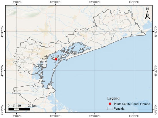
Figure 1.
Geographical location of the Venice Lagoon and the Punta Salute Canal Grande tidal station.

Figure 2.
Punta Salute station, Grand Canal.
2.2. Methods
2.2.1. Bidirectional Long Short-Term Memory Network
Traditional recurrent neural networks (RNNs) are susceptible to the problems of gradient explosion and gradient vanishing, making it difficult to capture long-range dependencies. Long Short-Term Memory (LSTM) networks [28], a variant of recurrent neural networks (RNNs), introduce a gating mechanism to regulate the flow of information, thereby addressing the issue of long-range dependencies inherent in traditional RNNs [29]. The structure of the LSTM network is illustrated in Figure 3.
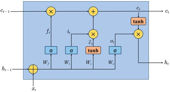
Figure 3.
The recurrent unit structure of the LSTM network.
The LSTM network introduces an internal state, denoted as , to enable linear recurrent information flow. The cell state retains historical information up to time step and serves as the long-term memory component of the LSTM architecture. The cell state transmits information to the external hidden state through a nonlinear transformation. represents the candidate state obtained through a nonlinear function. The formulations for the internal state, external state, and candidate state are as follows [30]:
where and represent the previous cell and hidden states, respectively; and are the weight matrices of the tanh activation layer in the input gate; is the bias term of the output gate; , , and are the three gates that control the information flow; tanh is a nonlinear activation function; represents the input at the current time step; and is the element-wise product of the vectors.
The LSTM network comprises three gates: the forget gate , the input gate , and the output gate . The forget gate is responsible for discarding irrelevant information from the previous cell state ; the input gate determines how much of the candidate state should be retained; and the output gate controls the amount of information from the current cell state that is passed to the hidden state . The corresponding equations are as follows [30]:
where , , and , along with , , and , are the weight matrices; , , and are the corresponding bias terms; and is a nonlinear activation function.
The computation process of the LSTM network is as follows: At each time step, the three gates (forget gate , input gate , and output gate ) are computed based on the current input and the previous external state . Next, the candidate state is calculated. The internal state is then updated by taking into account the forget gate and input gate . Finally, the output of the LSTM network is computed through the output gate .
Graves and Schmidhuber proposed the Bidirectional Long Short-Term Memory (BiLSTM) network [31]. The BiLSTM network consists of two layers of LSTM networks: one processes information in the forward temporal direction, while the other processes it in reverse. This bidirectional structure enables the model to capture both past and future context simultaneously, thereby providing a comprehensive understanding of temporal dynamics and enhancing the network’s representational capacity. The outputs of the forward and backward LSTM layers are integrated—either through concatenation or weighted averaging—to form the final output of the BiLSTM network. The BiLSTM model outperforms the standard LSTM in terms of accuracy and stability. To more effectively capture the nonlinear characteristics and long-term dependencies of tidal signals and to improve prediction accuracy, this study adopts the BiLSTM network as the predictive model. The structure of the BiLSTM network is illustrated in Figure 4.
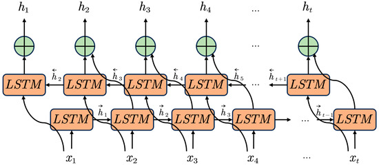
Figure 4.
BiLSTM structure.
The formula for BiLSTM is as follows [30]:
where and represent the external states of the forward propagation at time steps t and t−1, respectively; and represent the external states of the backward propagation at time steps and , respectively; represents the forward LSTM layer; represents the backward LSTM layer; and represent the internal states at time steps and , respectively; and denotes the input at time step .
The external hidden state of BiLSTM is formed by combining the outputs and from the forward and backward LSTM layers, respectively.
2.2.2. Successive Variational Mode Decomposition
The Successive Variational Mode Decomposition (SVMD) algorithm is a powerful decomposition method that extracts modes sequentially, overcoming the limitation of Variational Mode Decomposition (VMD), which requires a predefined number of modes K [24]. SVMD produces modes that are nearly identical to those of VMD while also offering lower computational complexity and higher robustness. This method can decompose complex, non-stationary tidal signals into a set of intrinsic mode functions (IMFs) that are simpler and physically meaningful, facilitating tidal analysis and providing a solid data foundation for further research.
SVMD decomposes the original signal into two components: the Lth mode and the residual signal .
The residual signal consists of two parts: the sum of the previously extracted modes , and the remaining unprocessed signal .
SVMD performs signal decomposition based on four criteria.
- (1)
- Each mode should be compactly concentrated around its center frequency.
This criterion requires minimizing the objective function for the Lth mode, ensuring that its frequency spectrum is most concentrated at the corresponding center frequency.
where is the center frequency of the Lth mode, * denotes the convolution operation, is the partial derivative with time t, and is the Dirac function.
- (2)
- The energy of the residual signal at frequencies where has significant components should be minimized.
To reduce spectral overlap between the residual signal and the target mode, the energy of the residual signal at frequencies where the Lth mode has effective components should be minimized. This is achieved by minimizing the objective function . SVMD employs a filter to attenuate the energy of the residual signal near the mode’s frequency band.
The frequency response of the filter is given by:
where is the center frequency of the Lth mode and α is a tuning parameter that controls the bandwidth of the filter.
The objective function is defined as:
where is the impulse response of the filter .
- (3)
- The energy of near the center frequencies of the previously extracted modes should be minimized.
SVMD defines the objective function to quantify the spectral overlap between the Lth mode and the previously extracted L−1 modes. By minimizing , the spectral overlap is reduced, ensuring spectral independence among the modes. This constraint is enforced by introducing specific frequency response filters .
The frequency response of is given by:
where is represented as follows:
where is the impulse response of the filter .
- (4)
- Ensure that all extracted modes and untreated signal components can be fully reconstructed to recover the original signal .
The formula for the reconstructed signal is:
where is the currently extracted Lth mode, denotes the unprocessed part of the signal, and represents the sum of the previously extracted L−1 modes.
Therefore, when the first L-1 modes are known, the extraction of the Lth mode can be formulated as a constrained minimization problem:
The parameter α is a balancing factor, which can be solved using the method of Lagrange multipliers.
The SVMD combines the quadratic penalty term and Lagrange multipliers to form the augmented Lagrangian function.
According to Parseval’s theorem, the above equation can be transformed into its frequency domain form.
SVMD uses the alternating direction method of multipliers (ADMM) [32] to iteratively solve the above minimization problem. The final iterative update equation is as follows:
where signifies the Fourier transform of the , is the Fourier transform of the Lth mode in the n-th repetition with the center frequency, n is the number of repetitions, t is the iteration step length, and τ is the update step size that controls the rate of change of the multipliers.
In signal decomposition, the number of modes K is a crucial parameter. If K is either too large or too small, it can negatively impact the quality of the decomposition. It is essential to determine the appropriate value of K in order to accurately capture the characteristics of tidal signals. Since different tidal signals exhibit distinct features, the optimal value of K may vary accordingly. VMD is a commonly used and powerful decomposition method that requires the specification of the parameter K [33]. When applying VMD to process tidal signals, conducting multiple experiments to determine the appropriate value of K is a necessary step, which can lead to increased algorithmic complexity. However, SVMD is able to directly perform decomposition on tidal signals without the need to set K, reducing the reliance on manual analysis. Additionally, its decomposition performance is comparable to that of VMD and can accurately capture the features of tidal signals. Therefore, this study utilizes SVMD to decompose tidal signals and extract their characteristic features.
2.2.3. SVMD-BiLSTM-Residual Decomposition
Tidal signals exhibit non-stationary characteristics due to geomorphological and meteorological factors. In regions with complex topography and highly variable weather conditions, tidal components are more intricate, making high-precision prediction more challenging. Currently, some high-precision tidal prediction models have high algorithmic redundancy to improve prediction accuracy, or they suffer from incomplete consideration of factors influencing tidal height. In response to these issues, this study combines SVMD and BiLSTM to propose the tidal prediction algorithm SVMD-BiLSTM-Residual Decomposition (SBRD). The overall framework of the specific prediction model is shown in Figure 5.
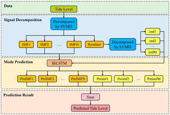
Figure 5.
SBRD structure.
SBRD utilizes SVMD to decompose the non-stationary and complex tidal data into locally stationary IMFs with clear physical meanings and distinct frequencies. These modes represent the influencing factors of astronomy, geology and landforms, meteorology, and other related aspects. The IMFs serve as the input to the BiLSTM network. SVMD separates the different frequency components of the tidal signal, reducing the signal complexity. This allows the model to better capture the signal features, facilitating improved learning and prediction. The IMFs with physical significance serve as inputs, effectively incorporating various factors that influence tidal levels into the analysis. This more comprehensive consideration contributes to improved prediction accuracy.
SBRD utilizes SVMD for two decompositions. The first decomposition is applied to the original tidal signal, resulting in multiple IMFs and a residual. The second decomposition is applied to the residual, which is the difference between the sum of the modes and the original signal, representing the remaining part after signal decomposition. This residual still contains information that influences tidal water levels. To enhance tidal forecasting accuracy, it is necessary to consider the information contained in the residual during the prediction process. Therefore, this model incorporates the residual into the model input. To improve the prediction accuracy of the complex residual, the same SVMD decomposition process is applied to the residual.
In SVMD, the coefficient α plays a crucial role in balancing the parameters during the optimization process. It is responsible for maintaining a balance between the compactness of the signal and the separation degree of the modes during the decomposition process. However, if α is too large, it can result in erroneous noise modes, which can significantly affect the convergence of the algorithm. On the other hand, if α is too small, it can lead to mode mixing [34]. To address this issue, the value of α is dynamically adjusted during the iteration process. Initially, it is set to αmin and then increases exponentially, but it is limited to not exceed the maximum value (αmax) that is set. This adjustment method helps the algorithm to identify the strongest modes during the iteration while avoiding any issues caused by excessively high or low values of α.
SBRD consists of three steps:
- (1)
- Signal Decomposition: The nonlinear and non-stationary tidal signal is decomposed into N IMFs and a residual signal using SVMD. The residual signal is then subjected to a second decomposition using SVMD, resulting in M IMFs. These N+M modes serve as the input to the BiLSTM network, providing a solid data foundation for the model’s prediction.
- (2)
- Data Prediction: The modes are independently predicted through the BiLSTM network, yielding several mode prediction results. The BiLSTM network captures both forward and backward information, allowing for a more comprehensive capture of the mode features. Additionally, simpler modes are easier for the model to learn, thereby improving prediction accuracy and stability.
- (3)
- Data Reconstruction: Finally, the predicted values of the modes are summed to reconstruct the final tidal prediction result.
2.3. Training Methods
2.3.1. Development Tools and Environment
The model development in this experiment is based on the Python deep learning framework TensorFlow. The Python version used is 3.9.20, and the TensorFlow version is 2.15.0. The CPU used is an Intel(R) Core (TM) i7-9750H CPU @ 2.60GHz, with 12 GB RAM. The operating system is Windows 10. Other software package versions used are numpy 1.26.0 and pandas 1.3.0.
The parameters of SVMD are shown in Table 1, and the training parameters of BiLSTM are shown in Table 2.

Table 1.
SVMD parameters.
Table 2.
BiLSTM training parameters.
2.3.2. Performance Evaluation Metrics
This study uses the Coefficient of Determination (R2), Mean Absolute Error (MAE), and Root Mean Square Error (RMSE) as metrics to evaluate the accuracy of tidal predictions.
R2 measures the degree of fit of the model to the data, with a range between 0 and 1. A value closer to 1 indicates a better fit. In this study, R2 is considered the indicator of prediction accuracy, and its formula is as follows:
MAE is the average of the absolute errors between the actual and predicted values, directly measuring the average difference between the predicted and actual values. A smaller MAE indicates better prediction performance. Its formula is as follows:
Mean Squared Error (MSE) is calculated by finding the average of the squared differences between the actual and predicted values. This metric is particularly sensitive to large errors and penalizes larger discrepancies. However, the output of MSE is in the square of the original units, making it less easily interpretable. RMSE is the square root of MSE, which eliminates the effect of units and presents the error in the same original units as the data. This makes it more intuitive when interpreting errors. The formula for RMSE is as follows:
In Equations (25)–(27), n represents the number of tidal level values, denotes the true value of the i-th tidal level, represents the predicted value of the i-th tidal level, and is the mean of the actual tidal level values.
3. Results
3.1. Tide Datasets Processing and Analysis
Figure 6 displays the tidal data for Punta Salute Canal Grande from 01:00:00 on 1 January 2018 to 12:00:00 on 29 December 2018. Figure 6 reveals three instances of abnormal tidal levels between March and April, with tidal heights around 1.2 m. Additionally, extreme tidal levels were recorded on 28 October and 29 October, with the highest reaching over 1.5 m. On November 24, a high tide occurred, reaching 1.14 m.
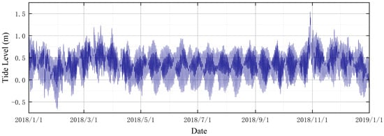
Figure 6.
Tidal Levels of Punta Salute Canal Grande in 2018.
The tidal dataset selected for this study was decomposed into six modes and a residual using the SVMD algorithm. The residual was then subjected to a second decomposition using SVMD, resulting in 19 modes. These 26 modes served as the input for the neural network. Figure 7 shows the time-domain plots of the 6 modes and one residual decomposed from the original tidal signal. Figure 8 presents the Fourier spectra of the 6 modes of the original signal. Figure 9 and Figure 10 show the time-domain plots and Fourier spectra of the 19 modes decomposed from the residual, respectively.
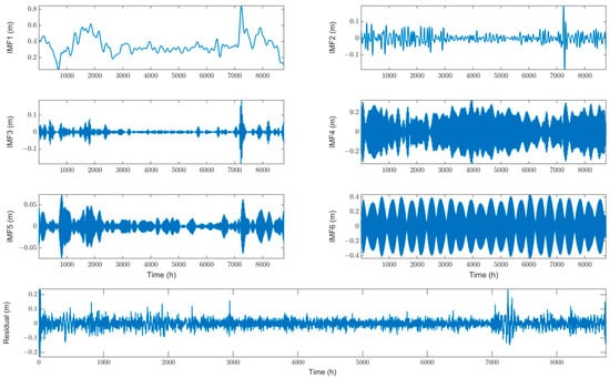
Figure 7.
The 6 modes and residual of the tidal levels at Punta Salute Canal Grande station in 2018.
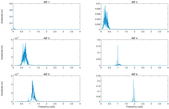
Figure 8.
Fourier spectra of the tidal level modes at Punta Salute Canal Grande station in 2018.
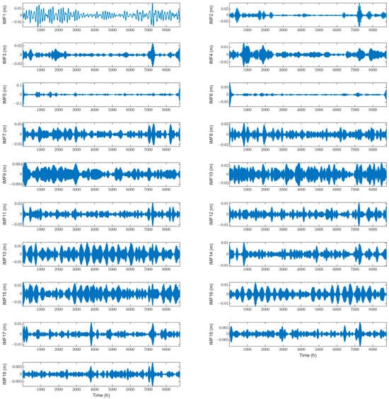
Figure 9.
The 19 modes of the water level residual at Punta Salute Canal Grande station in 2018.
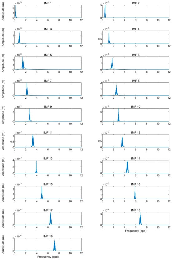
Figure 10.
Fourier spectra of the residual modes of the tidal levels at Punta Salute Canal Grande station in 2018.
Table 3 presents the mean amplitude and period of the SVMD modes for the 2018 Punta Salute station, Grand Canal tidal level. Among the six modes decomposed by SVMD, IMF1 has an average period of 8.631 days and an average amplitude of 0.3535 m, which is consistent with the trend and magnitude of the original tidal sequence. It represents sub-tidal oscillations, reflecting the large-scale fluctuations and low-frequency trends in the original tidal signal. IMF4 has an average period of 23 h and 42 min and an average amplitude of 0.1142 m, indicating that it represents the diurnal tide. Similarly, IMF6 has an average period of 12 h and 20 min and an average amplitude of 0.1705 m, indicating that it represents the semidiurnal tide. These relatively large average amplitudes make IMF4 and IMF6 the main contributors to tidal fluctuations. IMF5 has an average period of 20 h and an average amplitude of 0.0102 m. This period falls between the diurnal and semidiurnal tides, indicating a mixed tide resulting from the interaction of different tidal components. The average amplitude is relatively small, only around 1 cm, suggesting that it does not have a significant impact on tidal fluctuations and has a minor influence on tidal variations. IMF2 and IMF3 have average periods of 3.3 days and 1.4 days, with average amplitudes of 0.0209 m and 0.0110 m, respectively. Both of these modes have periods longer than one day, and their average amplitudes range between 1 and 2 cm. While they do not dominate tidal fluctuations, they do have some effect on tidal levels. Therefore, these two modes likely represent the influence of meteorological factors, such as wind fields, air pressure, and oceanic conditions, on tidal levels.
Table 3.
Mean amplitudes and periods of the tidal level modes at Punta Salute station, Grand Canal in 2018.
Overall, the SVMD method decomposes the tidal signal into several components: a low-frequency trend (IMF1), two astronomical-dominant components (IMF4, IMF6), a mixed tide component (IMF5), and two environmental factor components (IMF2, IMF3). This decomposition successfully decomposes the tidal signal into physically meaningful modes, effectively capturing its main characteristics and avoiding mode mixing, which makes learning and prediction easier.
Figure 8 and Figure 10 show the Fourier spectra of the original signal modes and residual modes, respectively. The spectra clearly indicate that oscillations at different time scales are strictly separated into different modes, with no mode mixing observed. This suggests that SVMD has successfully extracted the complex tidal features.
3.2. Prediction Results and Model Comparison
We use a data sampling interval of 1 h in this study. The SBRD algorithm predicts tidal level for the next 1, 3, 6, 12, and 24 h using the tidal levels from the past 10, 12, 18, 22, and 24 h, respectively. To demonstrate the advantages of the SBRD algorithm, five other models are introduced for comparison in this experiment: LSTM, BiLSTM, SVMD-BiLSTM, CEEMDAN-BiLSTM, and SVMD-BiLSTM-Residual. All six models are kept with consistent parameters.
LSTM is a widely used deep learning model for predicting time series data that can effectively handle the issue of long-range dependencies in RNNs. BiLSTM consists of two independent LSTM networks, combining both forward and backward directional information from the time series. In this experiment, we compare the BiLSTM and LSTM models to determine if the bidirectional model, BiLSTM, can improve prediction accuracy in tidal forecasting.
EMD and EEMD are classical signal decomposition algorithms, while CEEMDAN is an improved version of EEMD that incorporates adaptive noise. During each decomposition, CEEMDAN adaptively adjusts the noise intensity based on the characteristics of the signal, reducing errors caused by noise and enhancing the accuracy of signal decomposition. This method is more effective in eliminating the mode mixing problem. In this experiment, we compare CEEMDAN with SVMD to investigate whether SVMD can effectively improve tidal prediction accuracy compared to other decomposition algorithms. Table 4 shows the performance metrics of SBDR and the other five models’ prediction results. Figure 11 displays a comparison of R2, MAE, and RMSE for SBDR and the other five models, with the horizontal axis representing the prediction time.
Table 4.
Comparison of prediction performance across models.
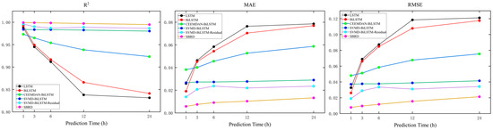
Figure 11.
Evaluation metric curves of different models.
As shown in Table 4, as the prediction time increases, the R2 of LSTM decreases from 0.98756 to 0.83150, the MAE increases from 2.5945 cm to 7.8578 cm, and the RMSE increases from 3.2749 cm to 12.10956 cm. Similarly, the R2 of BiLSTM decreases from 0.9921 to 0.8412, the MAE increases from 1.91315 cm to 7.69686 cm, and the RMSE increases from 2.60698 cm to 11.75646 cm. The evaluation metric curves (Figure 11) clearly show that BiLSTM outperforms the unidirectional LSTM model, with a higher R2 and lower MAE and RMSE values. This demonstrates that in the estimation of tidal level time series signals, the bidirectional model BiLSTM can capture information more comprehensively, providing better tidal estimation results. BiLSTM performs excellently in single-step prediction, with high accuracy and small errors. However, as the prediction time increases, its performance deteriorates. Therefore, this study combines BiLSTM with decomposition algorithms to improve the algorithm’s performance.
The CEEMDAN-BiLSTM and SVMD-BiLSTM models integrate the decomposition algorithms CEEMDAN and SVMD, respectively, into the BiLSTM model. CEEMDAN decomposes the tidal data into 15 modes, while SVMD decomposes the tidal data into 6 modes. As the prediction time increases, the R2 of CEEMDAN-BiLSTM decreases from 0.97318 to 0.923377, the MAE increases from 3.8214 cm to 5.8735 cm, and the RMSE increases from 4.80807 cm to 7.54927 cm. Similarly, the R2 of SVMD-BiLSTM decreases from 0.98395 to 0.9802, the MAE increases from 2.6705 cm to 2.9015 cm, and the RMSE increases from 3.71 cm to 4.14745 cm. The evaluation metric curves show that after incorporating the decomposition algorithm, the multi-step prediction performance of BiLSTM significantly improves, especially for SVMD-BiLSTM. The R2 values are above 0.98, the MAE does not exceed 3 cm, and the RMSE is around 3 to 4 cm. Although CEEMDAN-BiLSTM shows some improvement compared to BiLSTM, its performance enhancement is not as significant as that of SVMD-BiLSTM. This indicates that SVMD can more accurately extract the features of the signal, reduce the signal’s complexity, and provide a better data foundation for the prediction model, thereby enhancing prediction accuracy.
However, in single-step prediction, the prediction performance of BiLSTM with the added decomposition algorithm decreases rather than improves. The reasons for this are analyzed as follows: First, single-step prediction focuses on information within a short time frame, avoiding the uncertainty and cumulative errors present in long-term predictions. Moreover, BiLSTM performs well in single-step prediction, achieving high accuracy in such tasks. Secondly, SVMD-BiLSTM and CEEMDAN-BiLSTM do not take the residual’s impact into account during the prediction process, while the residual still contains useful uncaptured information. The absence of this information leads to slightly poorer performance for SVMD-BiLSTM in single-step prediction compared to BiLSTM.
In addition to the modes, the SVMD-BiLSTM-Residual model also incorporates the residual as an input to the neural network. In single-step prediction, the R2 of SVMD-BiLSTM-Residual is 0.995821, the MAE is 1.419 cm, and the RMSE is 1.8979 cm. Compared to BiLSTM, the R2 improved by 0.3734%, the MAE decreased by 0.494 cm, improving by 25.83%, and the RMSE decreased by 0.709 cm, improving by 27.2%. The purple line in Figure 11 represents the prediction results of SVMD-BiLSTM-Residual. It can be seen that, in addition to the improvement in single-step prediction, the performance of multi-step prediction also shows some enhancement compared to SVMD-BiLSTM, which does not consider the residual.
Due to the complexity of the components of the residual, the prediction performance is generally limited. In order to further improve prediction accuracy, the SBRD model uses SVMD to decompose the residual signal into 19 modes. Each of these 19 modes is then predicted separately using BiLSTM, and the mode prediction results are reconstructed to obtain the residual prediction results. The orange line in Figure 11 represents the prediction results of SBRD. From the chart, it can be observed that, whether for single-step or multi-step prediction, SBRD has the smallest prediction errors, the highest accuracy, and the best fit compared to the other models. The R2 reaches over 99%, the MAE ranges from 0.5806 cm to 1.3319 cm, and the RMSE ranges from 0.7803 cm to 2.1286 cm. Compared to the initial BiLSTM model, SBRD shows significant improvements in prediction accuracy, with an increase in R2 of 0.7231%, 5.2124%, 8.9055%, 15.1641%, and 18.2569% for 1, 3, 6, 12, and 24 h predictions, respectively. The MAE of SBRD decreases by 69.6522%, 83.4889%, 83.2590%, 85.3004%, and 82.6955%, respectively, while the RMSE decreases by 70.0688%, 85.5191%, 86.1808%, 85.5893%, and 81.8942%.
3.3. Twenty-Four-Hour Ahead Prediction of Extreme Tidal Levels
Reliable tidal forecasting is crucial for safeguarding Venice and its lagoon from the effects of high tidal levels. In order to provide enough time for evacuation and property relocation, a 24 h advance forecast is necessary.
Table 5 displays the evaluation metrics for the tidal prediction results at the 24th hour. Out of the six models, SBRD demonstrates the highest accuracy and the smallest errors, with an R2 of 98.679%, an MAE of 2.2246 cm, and an RMSE of 3.3976 cm.
Table 5.
Comparison of prediction performance across models for the 24 h tidal level prediction.
From 29 October to 30 October 2018, extreme tidal levels were recorded at the Punta Salute Canal Grande tidal station. On 28 October, a high tide of 1.21 m was observed at 13:00, followed by a high tide of 1.54 m at 15:00 on 29 October. A third abnormal high tide occurred at 20:00 on 29 October, reaching 1.41 m. Figure 12 is a curve chart displaying the 24 h predicted and actual values for the period of 28 October to 30 October, using six models. The pink line represents the actual values. It can be seen that the LSTM and BiLSTM models have errors of several tens of centimeters compared to the actual values, with larger errors occurring near extreme tidal levels. The maximum error reaches around 1 m. After incorporating the decomposition algorithm, the prediction error of BiLSTM decreases. However, the CEEMDAN-BiLSTM model shows significant prediction errors after 29 October, with its rising and falling trends not matching the actual tidal trends. The three algorithms that combine BiLSTM with SVMD show significant improvements in prediction accuracy, with the rising and falling trends aligning well with the actual tidal trends. In particular, the SBRD model has the highest fit, with the smallest prediction errors for extreme tidal levels. The 24 h ahead prediction error is around 3 cm. The prediction error for the first 1.21 m extreme tide is 7.318 cm, while the prediction error for the second 1.54 m extreme tide is 11.335 cm. The prediction error for the third observed abnormal tide, a few hours later, is even lower at 4.188 cm, proving that the SBRD model can provide highly accurate tidal forecasts within 24 h.
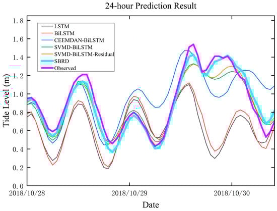
Figure 12.
Comparison of 24 h tidal level prediction results of different models during the 28–30 October 2018 period.
On 1, 4, 5, and 24 November of 2018, abnormal tidal levels exceeding 1 m were also recorded, although they were less extreme than the abnormal tides observed from 28 to 29 October 2018. Figure 13 illustrates the 24 h predictions and observations from six models during these events. Among them, the SBRD model exhibited the best fit and the smallest errors, thereby providing further evidence of its effectiveness in predicting and responding to extreme tidal conditions.
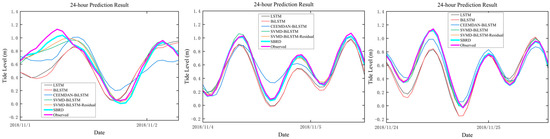
Figure 13.
Comparison of 24 h tidal level prediction results of different models during three extreme tidal events.
4. Discussion
4.1. Challenges in Tidal Prediction
Current tidal prediction methods can be broadly categorized into traditional analytical approaches, numerical simulations, and machine learning techniques. Traditional methods, such as harmonic analysis (HA), represent tides as a linear combination of sinusoidal waves with different frequencies, amplitudes, and phases. However, this approach assumes that tides are stationary signals with constant amplitudes and phases, which is only applicable in regions with minimal non-astronomical tidal influences. In areas with complex topography, atmospheric forcing, and other environmental factors, tides are non-stationary and traditional methods may not be suitable.
While numerical simulations can accurately forecast non-stationary tides, they require extensive computational resources. In contrast, machine learning and artificial intelligence have shown strong potential in modeling complex natural phenomena, offering a new direction for overcoming the challenges of prediction accuracy and computational demand faced by traditional models. As tidal levels are inherently time series signals, many researchers have adopted models such as LSTM and BiLSTM for tidal forecasting, achieving promising results. However, there are still several challenges in applying deep learning methods to tidal prediction, including the need for large amounts of historical tidal data, high model complexity, and insufficient consideration of diverse influencing factors.
Accordingly, one of the main challenges in tidal prediction is finding a balance between maintaining high forecasting accuracy, controlling model complexity, and reducing reliance on extensive historical tidal records. The value of tidal forecasting lies in its ability to provide early warning and preparedness for a variety of maritime and coastal activities. In particular, extreme tidal events are highly destructive and difficult to predict, making the accurate prediction of extreme tidal levels a critical and urgent issue in the field of tidal prediction.
4.2. Advantages of SBRD
Previous studies have utilized various deep learning models for tidal prediction. However, some of these studies have limitations, such as not fully considering non-astronomical factors. For example, Bai and Xu (2021) used a Bi-LSTM model and achieved an R2 of 0.9647 in 24 h forecasts, but they did not fully consider non-astronomical factors or extreme tidal events [1]. Similarly, Zhang et al. (2023) proposed a graph convolutional recurrent network, which achieved an RMSE of 0.158 m and MAE of 0.121 m for 12 h forecasts, but the method relied heavily on large historical datasets [2]. In contrast, Raidan Bassah et al. (2025) developed a ConvLSTM model with comparable accuracy to local models, but the training process was computationally expensive [14]. Another study by Liao et al. (2025) introduced an EMD-MLP hybrid model that showed high short-term accuracy, but the use of EMD may lead to mode mixing and end effects [20].
In this paper, we propose an innovative tidal prediction model called SBRD, which combines the SVMD decomposition algorithm and the BiLSTM network. Our study focuses on Venice, a city that frequently experiences extreme tidal events, such as “acqua alta”. We collected 8700 sea level height samples from the Punta Salute Canal Grande tidal station in Venice from 2018 to create our dataset. The SBRD model uses SVMD to decompose the nonlinear and non-stationary tidal signal into six modes and one residual. The residual is then subjected to a second decomposition using SVMD, resulting in 19 modes. This approach effectively separates the tidal signal into components on different time scales. The complex tidal signal is decomposed into multiple modes with local stationarity, low complexity, and strong periodicity, capturing more precise tidal features. Finally, the modes are predicted separately using the BiLSTM network, and the predicted results are aggregated to obtain the final tidal prediction.
This study predicts tidal levels for the next 1, 3, 6, 12, and 24 h, and the experimental results are as follows:
- (1)
- The SBRD model exhibits the smallest prediction error, highest accuracy, and best fitting compared to other models, for both single-step and multi-step predictions. The tidal predictions within 24 h achieve an R2 of over 99%, with MAE errors ranging from 0.5806 cm to 1.3319 cm, and RMSE errors ranging from 0.7803 cm to 2.1286 cm.
- (2)
- In the prediction results for the 24th hour tidal level, the SBRD model shows the highest accuracy and the smallest error, with an R2 of 98.679%, an MAE of 2.2246 cm, and an RMSE of 3.3976 cm. During the period from October 9 to October 30, 2018, three extreme tidal levels occurred. The SBRD model provided the best fit for the predictions during this period. In the 24 h ahead predictions, the error for the first abnormal tidal level of 1.21 m was 7.318 cm, the error for the second extreme tidal level of 1.54 m was 11.335 cm, and the error for the third abnormal tidal level of 1.41 m was 4.188 cm. These results demonstrate that the SBRD model can achieve high-precision predictions for tidal levels within the next 24 h, even in the presence of extreme tidal events.
The proposed SBRD model, applied to tidal forecasts in Venice, achieved R2 values exceeding 99%, with MAE values within 1.3319 cm and RMSE values within 2.1286 cm for predictions within 24 h. Compared to other models, SBRD demonstrated superior performance in accurately predicting tides under complex conditions. The dataset used consisted of 8700 sea level samples over the course of one year, reducing the need for extensive historical records. In Section 3.1, the SVMD-based tidal data processing is presented. The decomposed modes are found to be simpler, more stationary, and physically interpretable, without any mode mixing. This indicates that SVMD successfully captured the primary tidal features. In Section 3.3, the 24 h forecast is analyzed, with SBRD achieving an R2 of 98.679%, an MAE of 2.2246 cm, and an RMSE of 3.3976 cm. This confirms the model’s ability to accurately predict tides within a 24 h period. Further analysis of four periods with extreme tidal levels (Figure 12 and Figure 13) shows that the predictions of SBRD exhibit a high degree of agreement with the observed values and yield small errors in forecasting extreme values. This demonstrates the model’s robustness in handling extreme tidal events.
5. Conclusions
In summary, this study develops the SBRD model by integrating SVMD decomposition with BiLSTM networks for tidal prediction in Venice. The model achieves high-accuracy forecasts, demonstrates robustness in handling extreme tidal events, and provides practical implications for marine economic development and disaster prevention.
While the SBRD model achieves satisfactory accuracy in tidal predictions within 24 h, there is still room for improvement. The model currently only predicts tidal levels for a single station and cannot simultaneously estimate tidal levels for multiple stations in a region. Therefore, the model’s generalizability needs to be enhanced. In future research, we plan to analyze the interrelationships between tidal levels at different stations and upgrade from single-point temporal prediction to spatiotemporal prediction, allowing for regional tidal forecasting without sacrificing accuracy.
Author Contributions
Conceptualization, L.Z., Y.F. and C.N.; methodology, L.Z., H.L. and C.N.; software, L.Z.; validation, L.Z.; formal analysis, C.N. and W.S.; investigation, L.Z. and H.L.; resources, C.N., W.S. and H.L.; data curation, L.Z., C.N. and C.L.; writing—original draft, L.Z., C.N. and W.S.; writing—review and editing, Y.J., C.N. and Y.F.; visualization, L.Z. and W.S.; supervision, C.N., C.L. and Y.F., project administration, C.N.; funding acquisition, C.N. All authors have read and agreed to the published version of the manuscript.
Funding
This work was supported by the National Key Research and Development Program of China [2022YFC3104301].
Data Availability Statement
The data presented in this study are available in from the Comune di Venezia website at https://www.comune.venezia.it/it/content/1-punta-salute-canal-grande (accessed on 1 April 2025). These data were derived from the following resources available in the public domain: National Research Council Institute of Marine Sciences (IS-MAR-CNR) (https://www.comune.venezia.it/it [accessed on 1 April 2025]). [Comune di Venezia website] [https://www.comune.venezia.it/it/content/1-punta-salute-canal-grande (accessed on 1 April 2025)].
Conflicts of Interest
The authors declare no conflict of interest.
Abbreviations
The following abbreviations are used in this manuscript:
| VMD | Variational Mode Decomposition |
| SVMD | Successive Variational Mode Decomposition |
| IMF | Intrinsic Mode Function |
| WT | Wavelet Transform |
| EMD | Empirical Mode Decomposition |
| EEMD | Ensemble Empirical Mode Decomposition |
| CEEMDAN | Complete Ensemble Empirical Mode Decomposition with Adaptive Noise |
| R2 | Coefficient of Determination |
| MSE | Mean Squared Error |
| RMSE | Root Mean Squared Error |
| MAE | Mean Absolute Error |
| HA | Coefficient of Determination |
| WA | Coefficient of Determination |
| SWAN | Simulation of Waves in the Nearshore |
| ADCIRC | Advanced Circulation Model |
| Delft3D | Delft 3D Flow Model |
| FVCOM | Finite Volume Community Ocean Model |
| RNN | Recurrent Neural Network |
| LSTM | Long Short-Term Memory |
| BiLSTM | Bidirectional Long Short-Term Memory |
| BALSSA | Bidirectional Attention-based LSTM Storm Surge Architecture |
| RMSTL | Regional Multi-Station Tide-Level Prediction Model |
| MOSE | MOdulo Sperimentale Elettromeccanico—Experimental Electromechanical Module |
| ADMM | Alternating Direction Method of Multipliers |
References
- Bai, L.H.; Xu, H. Accurate estimation of tidal level using bidirectional long short-term memory recurrent neural network. Ocean. Eng. 2021, 235, 108765. [Google Scholar] [CrossRef]
- Zhang, X.; Wang, T.; Wang, W.; Shen, P.; Cai, Z.; Cai, H. A multi-site tide level prediction model based on graph convolutional recurrent networks. Ocean. Eng. 2023, 269, 113579. [Google Scholar] [CrossRef]
- Pan, H.; Lv, X.; Wang, Y.; Matte, P.; Chen, H.; Jin, G. Exploration of tidal-fluvial interaction in the Columbia River estuary using S_TIDE. J. Geophys. Res. Ocean. 2018, 123, 6598–6619. [Google Scholar] [CrossRef]
- Dietrich, J.C.; Tanaka, S.; Westerink, J.J.; Dawson, C.N.; Luettich, R.A., Jr.; Zijlema, M.; Holthuijsen, L.H.; Smith, J.M.; Westerink, L.G.; Westerink, H.J. Performance of the unstructured-mesh, SWAN + ADCIRC model in computing hurricane waves and surge. J. Sci. Comput. 2012, 52, 468–497. [Google Scholar] [CrossRef]
- Lenstra, K.J.; Pluis, S.R.; Ridderinkhof, W.; Ruessink, G.; van der Vegt, M. Cyclic channel-shoal dynamics at the Ameland inlet: The impact on waves, tides, and sediment transport. Ocean. Dyn. 2019, 69, 409–425. [Google Scholar] [CrossRef]
- Xianwu, S.; Yafei, L.; Dibo, D.; Ning, J.; Jianzhong, G.; Jie, Y. Quantitative assessment of building risks and loss ratios caused by storm surge disasters: A case study of Xiamen, China. Appl. Ocean. Res. 2024, 145, 103934. [Google Scholar] [CrossRef]
- Chen, B.F.; Wang, H.D.; Chu, C.C. Wavelet and artificial neural network analyses of tide forecasting and supplement of tides around Taiwan and South China Sea. Ocean. Eng. 2007, 34, 2161–2175. [Google Scholar] [CrossRef]
- Yang, C.H.; Wu, C.H.; Hsieh, C.M. Long short-term memory recurrent neural network for tidal level forecasting. IEEE Access 2020, 8, 159389–159401. [Google Scholar] [CrossRef]
- Ian, V.K.; Tang, S.K.; Pau, G. Assessing the risk of extreme storm surges from tropical cyclones under climate change using bidirectional attention-based LSTM for improved prediction. Atmosphere 2023, 14, 1749. [Google Scholar] [CrossRef]
- Shi, X.; Chen, P.; Ye, Z.; Zhang, X.; Wang, W. Tide level prediction during typhoons based on variable topology in graph convolution recurrent neural networks. Ocean. Eng. 2024, 312, 119228. [Google Scholar] [CrossRef]
- Kim, C.S.; Kok, K.H.; Kim, C.R. Quasi-Optimized LSTM Approach for River Water Level Forecasting. Water 2025, 17, 2087. [Google Scholar] [CrossRef]
- Lai, C.; Liao, Y.; Yu, H.; Wang, Z.; Liao, Y.; Yang, B.; Niu, Q.; Jiang, Z.; Li, X.; Xu, C.-Y. Formation mechanism analysis and the prediction for compound flood arising from rainstorm and tide using explainable artificial intelligence. J. Environ. Manag. 2025, 388, 125858. [Google Scholar] [CrossRef]
- Chang, Y.W.; Sun, W.; Kow, P.Y.; Lee, M.H.; Chang, L.C.; Chang, F.J. Advanced groundwater level forecasting with hybrid deep learning model: Tackling water challenges in Taiwan’s largest alluvial fan. J. Hydrol. 2025, 655, 132887. [Google Scholar] [CrossRef]
- Bassah, R.; Corzo, G.; Bhattacharya, B.; Haider, S.M.; Swain, E.D.; Aumen, N. Forecasting water levels using the ConvLSTM algorithm in the Everglades, USA. J. Hydrol. 2025, 652, 132195. [Google Scholar] [CrossRef]
- Kaya, Y. Slope-aware and self-adaptive forecasting of water levels: A transparent model for the Great Lakes under climate variability. J. Hydrol. 2025, 662, 133948. [Google Scholar] [CrossRef]
- Daubechies, I. The wavelet transform, time-frequency localization and signal analysis. IEEE Trans. Inf. Theory 2002, 36, 961–1005. [Google Scholar] [CrossRef]
- Huang, N.E.; Shen, Z.; Long, S.R.; Wu, M.C.; Shih, H.H.; Zheng, Q.; Yen, N.-C.; Tung, C.C.; Liu, H.H. The empirical mode decomposition and the Hilbert spectrum for nonlinear and non-stationary time series analysis. Proc. R. Soc. London. Ser. A Math. Phys. Eng. Sci. 1998, 454, 903–995. [Google Scholar] [CrossRef]
- Wu, Z.; Huang, N.E. Ensemble empirical mode decomposition: A noise-assisted data analysis method. Adv. Adapt. Data Anal. 2009, 1, 1–41. [Google Scholar] [CrossRef]
- Torres, M.E.; Colominas, M.A.; Schlotthauer, G.; Flandrin, P. A Complete Ensemble Empirical Mode Decomposition with Adaptive Noise. In Proceedings of the 2011 IEEE International Conference on Acoustics, Speech and Signal Processing (ICASSP), Prague, Czech Republic, 22–27 May 2011; IEEE: Piscataway, NJ, USA, 2011; pp. 4144–4147. [Google Scholar]
- Liao, S.; Wang, L.; Wang, S.; Jia, B.; Yin, J.; Li, R. Accurate tidal prediction based on empirical mode decomposition-enhanced multilayer perceptron. Ocean. Eng. 2025, 336, 121848. [Google Scholar] [CrossRef]
- Dragomiretskiy, K.; Zosso, D. Variational mode decomposition. IEEE Trans. Signal Process. 2013, 62, 531–544. [Google Scholar] [CrossRef]
- Gan, M.; Pan, H.; Chen, Y.; Pan, S. Application of the Variational Mode Decomposition (VMD) Method to River Tides. Estuar. Coast. Shelf Sci. 2021, 261, 107570. [Google Scholar] [CrossRef]
- Xie, K.; Zhang, T. Forecasting Significant Wave Height Intervals Along China’s Coast Based on Hybrid Modal Decomposition and CNN-BiLSTM. J. Mar. Sci. Eng. 2025, 13, 1163. [Google Scholar] [CrossRef]
- Nazari, M.; Sakhaei, S.M. Successive variational mode decomposition. Signal Process. 2020, 174, 107610. [Google Scholar] [CrossRef]
- Gačić, M.; Mosquera, I.M.; Kovačević, V.; Mazzoldi, A.; Cardin, V.; Arena, F.; Gelsi, G. Temporal variations of water flow between the Venetian lagoon and the open sea. J. Mar. Syst. 2004, 51, 33–47. [Google Scholar] [CrossRef]
- Reimann, L.; Vafeidis, A.T.; Brown, S.; Hinkel, J.; Tol, R.S. Mediterranean UNESCO World Heritage at risk from coastal flooding and erosion due to sea-level rise. Nat. Commun. 2018, 9, 4161. [Google Scholar] [CrossRef]
- Comune di Venezia. Centro Previsioni e Segnalazioni Maree-Dati e Statistiche-Rete Telemareografica_Dati Tempo Reale e Archivio-Punta Salute Canal Grande. 2020. Available online: https://www.comune.venezia.it/it/content/1-punta-salute-canal-grande (accessed on 1 April 2025).
- Hochreiter, S.; Schmidhuber, J. Long short-term memory. Neural Comput. 1997, 9, 1735–1780. [Google Scholar] [CrossRef]
- Bengio, Y.; Simard, P.; Frasconi, P. Learning long-term dependencies with gradient descent is difficult. IEEE Trans. Neural Netw. 1994, 5, 157–166. [Google Scholar] [CrossRef] [PubMed]
- Qiu, X. Neural Networks and Deep Learning; China Machine Press: Beijing, China, 2020. [Google Scholar]
- Graves, A.; Schmidhuber, J. Framewise phoneme classification with bidirectional LSTM and other neural network architectures. Neural Netw. 2005, 18, 602–610. [Google Scholar] [CrossRef] [PubMed]
- Boyd, S.; Parikh, N.; Chu, E.; Peleato, B.; Eckstein, J. Distributed Optimization and Statistical Learning via the Alternating Direction Method of Multipliers. In Foundations and Trends® in Machine Learning; Now Publishers Inc.: Hanover, MA, USA, 2011; Volume 3, pp. 1–122. [Google Scholar]
- Qi, G.; Zhao, Z.; Zhang, R.; Wang, J.; Li, M.; Shi, X.; Wang, H. Optimized VMD algorithm for signal noise reduction based on TDLAS. J. Quant. Spectrosc. Radiat. Transf. 2024, 312, 108807. [Google Scholar] [CrossRef]
- Parsaie, A.; Ghasemlounia, R.; Gharehbaghi, A.; Haghiabi, A.; Chadee, A.A.; Nou, M.R.G. Novel hybrid intelligence predictive model based on successive variational mode decomposition algorithm for monthly runoff series. J. Hydrol. 2024, 634, 131041. [Google Scholar] [CrossRef]
Disclaimer/Publisher’s Note: The statements, opinions and data contained in all publications are solely those of the individual author(s) and contributor(s) and not of MDPI and/or the editor(s). MDPI and/or the editor(s) disclaim responsibility for any injury to people or property resulting from any ideas, methods, instructions or products referred to in the content. |
© 2025 by the authors. Licensee MDPI, Basel, Switzerland. This article is an open access article distributed under the terms and conditions of the Creative Commons Attribution (CC BY) license (https://creativecommons.org/licenses/by/4.0/).