A Quantitative Evaluation Method for Navigation Safety in Coastal Waters Based on Unstructured Grids

Abstract

In this paper, we propose a quantitative evaluation method for navigation safety in coastal waters based on unstructured grids. Initially, a comprehensive analysis was conducted on various factors affecting navigation safety, including natural conditions, traffic conditions, and marine hydro-meteorological conditions, to construct a multi-source fused spatiotemporal dataset. Subsequently, channel boundary extraction was performed using Constrained Delaunay Triangle–Alpha-Shapes, and the precise extraction of ship navigation areas was performed based on Constrained Delaunay Triangle–Voronoi diagrams. Additionally, temporal feature grids were constructed based on the spatiotemporal characteristics of marine hydro-meteorological data. Finally, unstructured grids for evaluating navigation safety were established through spatial overlay analysis. Based on this foundation, a quantitative analysis and evaluation model for comprehensive navigation safety assessment was developed using the fuzzy evaluation method. By calculating the fuzzy relation matrix and weight vectors, quantitative assessments were conducted for each grid cell, yielding safety risk levels from both spatial and temporal dimensions. An analysis was performed using maritime data within the geographic boundaries of lon.119.17–120.41° E and lat.34.40–35.47° N. The results indicated that the unstructured grid division and channel boundary extraction in the demonstrated sea area were closely related to parameters such as the ship traffic flow patterns and the spatiotemporal characteristics of the marine environmental factors. A quantitative evaluation and analysis of the 186 unstructured grid cells revealed that the high risk levels primarily corresponded to restricted navigation areas, the higher-risk grid cells were mainly anchorages, and the low to lower risk levels were primarily associated with channels and navigable areas for ships.

1. Introduction

Shipborne navigation safety remains a critical focus area in maritime engineering research. Ship maneuvering safety is influenced by numerous internal and external factors, such as waves, tidal currents, and wind, which are important factors for safe and economic ship navigation [1]. Meanwhile, the long-term sustainability of seaports depends on various operational factors, including infrastructure efficiency, digital innovation, environmental management, and regulatory compliance, among which maritime pilotage plays a crucial role in ensuring safe navigation and minimizing environmental, economic, and social risks [2]. Firstly, the trend of larger ship sizes and frequent port entries and exits has led to an increase in channel traffic density, sometimes even exceeding channel capacity and resulting in congestion. Secondly, the intricate routing and navigational obstruction issues in coastal waters elevate the risks of ship grounding, running aground, and collisions. Thirdly, navigation is significantly affected by natural environmental factors such as marine hydrology and meteorology.

Geospatial grid technology, with grid partitioning as a common approach in marine research, faces challenges in dividing research objects into fine units and dynamically adjusting grids. Researchers have conducted relevant studies: Oje et al. [3] introduced the Hierarchical Grid Partitioning (HierGP) framework; Zhang et al. [4] designed a visualized intelligent management method for spatiotemporal grids; Li et al. [5] proposed a method of constructing non-uniform grids based on quadtrees; Zhu et al. [6] established a recursive system in the airspace; Liu et al. [7] designed a representation and conflict detection method for the traditional airspace; Ware et al. [8] designed a global geospatial grid system; environmental risks have been evaluated and zoned on a grid map by adopting the spatial analysis method [9]; An organization model of electromagnetic field data has been established based on subdivision grids [10]; and Hou et al. [11] proposed a dynamic partitioning method for road network areas.

With coastal development and environmental changes, creating high-quality computational grids and assessing their impacts are crucial. This has been achieved by many researchers, including the following: Bousquin [12] applied a hexagonal geospatial framework in coastal areas; Chen et al. [13] established an indicator system for the evaluation of geological environment stability; Ding et al. [14] applied a hexagonal discrete global grid system to the generation of depth contours; Wang et al. [15] conducted research on the extraction of hexagonal grid structures; Mou et al. [16] mined the sailing characteristics of ships; and Pringle et al. [17] conducted research on the sensitivity of global unstructured grid design. From the perspective of navigation safety risk assessment, researchers have also used quantitative methods: Zhang et al. [18] used Bayesian networks to estimate collision accident probability; Zhao et al. [19] combined fuzzy fault tree analysis with Bayesian networks; Aydin et al. [20] identified ship collision risks using Bayesian network methods; Wu et al. [21] developed a decision support model; Li et al. [22] developed a risk behavior simulation model; Ma et al. [23] studied the coupling relationship among risk factors; Bai et al. [24] proposed an improved gray clustering navigation safety evaluation model; Zhou et al. [25] proposed a method for the optimal selection of pilot boarding areas; Huang et al. [26] established a navigation safety evaluation model based on the game theory combination weighting method; He et al. [27] proposed an online prediction model for ship navigation risk; and researchers have also combined advanced methods to construct comprehensive evaluation models for navigation safety [28,29,30,31,32,33,34]. Garay-Rondero C L used the PRISMA ScR method to select relevant research resources, providing technical support for maritime boundary delineation, regulatory barriers, and other related areas [35].

In summary, geospatial grid technology has gradually evolved from regular grids to adaptive and irregular grids, enhancing the efficiency and accuracy of spatial data processing. In terms of dynamic grid partitioning, geospatial grid technology is gradually evolving from regular grids to adaptive and irregular grids, improving the efficiency and accuracy of spatial data utilization and providing support for navigation safety. However, research on dynamic irregular grids in maritime areas remains relatively scarce. There is a need to further develop refined dynamic irregular grid partitioning techniques tailored to the characteristics of maritime regions, in order to improve the grid’s analytical capabilities for complex maritime topography, ocean environments, and traffic flows. Additionally, it is essential to optimize grid partitioning algorithms to enhance computational efficiency and accuracy, thereby meeting the demands for maritime navigation safety. Most traditional navigation safety evaluation methods are either conducted for entire regions or based on regular grid models, making it difficult to effectively capture the local characteristics and dynamic change information of the navigation environment or identify potential risk areas and times.

Based on this, the research discussed in this paper involved the following: (1) Unstructured grids that reflected the characteristics of coastal waters were constructed to improve the grid’s comprehensive analysis capabilities for complex seabed topography, marine environments, and traffic flow, and the grid partitioning algorithm was optimized to improve computational efficiency and accuracy. (2) A comprehensive evaluation model that reflected comprehensive risk factors and dynamic change processes was developed, quantitative assessment calculations of the safety risks were conducted based on the partitioned unstructured grids, and the safety risk levels of each grid unit were analyzed. We constructed and comprehensively evaluated unstructured coastal water grids adapted to dynamic changes in the navigation environment, achieved using research on quantitative evaluation methods for ship navigation safety based on unstructured grids. This research has application value in addressing ship navigation safety risks and providing safety guarantees.

2. Methods

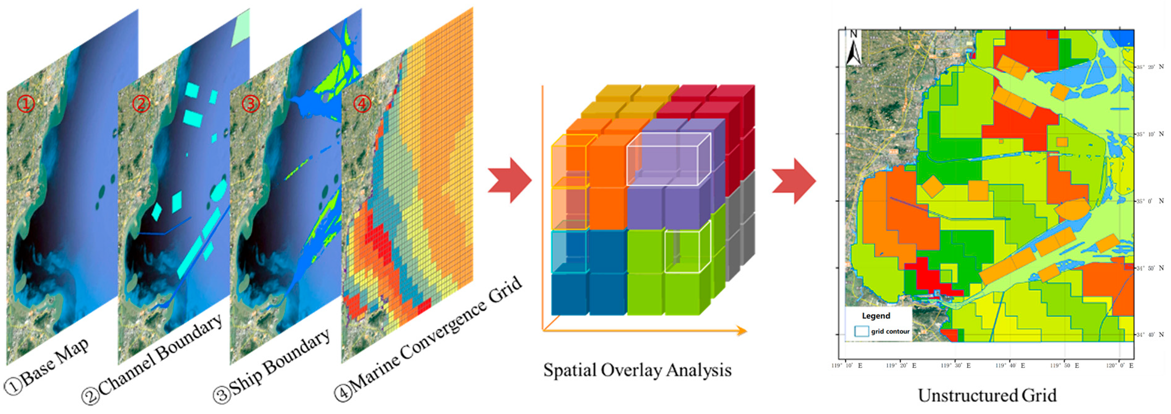
This paper focuses on a detailed discussion of unstructured grid division methods. Based on the analysis of factors such as natural environment, traffic, marine hydro-meteorological conditions, and the integration of data on basic geography, ship traffic flow, and marine environment, the process began by extracting the boundaries of port access channels using bathymetric survey data. Subsequently, large-scale ship scatter data were used to extract ship navigation boundaries. Spatial integration was then employed to form the overall navigation boundaries of coastal waters. Finally, spatial overlay analysis was conducted in combination with marine hydro-meteorological data to generate unstructured grids. Considering the temporal characteristics of the data elements, dynamic grids were generated on a time-based scale, providing basic data support for safety assessments and graphical references for the early warning and control of ship navigation risks. Figure 1 illustrates the specific process followed.

2.1. Materials

Underwater topography, electronic nautical charts, ship traffic flow, marine hydrology and meteorology data play a vital role in ensuring navigational safety. By fully leveraging these data resources and strengthening analytical and utilization capacity, it is possible to ensure comprehensive, precise, and real-time protection for ship navigation.

Underwater topography data is a digital collection that describes seabed geomorphological features, topographic measurements, and change monitoring, providing an intuitive reflection of coastal terrain characteristics. Based on the spatial distribution characteristics of the terrain, topographic factors influencing navigation are further extracted. Seafloor topography data is derived from periodic dredging surveys of navigation channels in the study area and integrated to construct a digital elevation model (DEM) of seabed depth, thereby digital simulation of marine terrain.

Electronic nautical chart (ENC) data is a digital product that describes geographic and navigational information of marine areas. It includes aids to navigation such as lighthouses and buoys, obstacles that may affect vessel navigation such as shipwrecks, underwater pipelines, and cables, as well as port facilities including docks, berths, and anchorages, together with information on channel width, depth, and curvature radius. These provide comprehensive information for navigational safety and effectively prevent potential hazards.

Ship traffic flow data is a series of digital information that describes the continuous movement of maritime traffic. The navigation patterns and characteristics of ships within a specific sea area can be understood by analyzing vessel traffic flow data. The processes of vessel entry and departure have accumulated a vast amount of vessel traffic flow data resources, covering eight categories of ships, including container ships, cargo vessels, and fishing boats. This study uses 48,372,968 dynamic vessel records from the research area.

Marine hydro-meteorological data is used to describe the state and variation patterns of hydrological and meteorological elements in the marine environment, including sea conditions such as wind, waves, and currents. The combined effect of multiple factors has a significant impact on the safe navigation of vessels. Vessels need to select appropriate routes and speeds based on sea condition information to ensure navigational safety.

The data used in this study area of this thesis are shown in

Table 1. The data elements used in the paper.

No.	Data Type	Data Item	Resolution/Scale	Data Organization Method
1	Underwater Topography Data	Surveyed Bathymetric Data	1:1000	Formatted Table
2	Electronic Nautical Chart Data	Channel Anchorage Restricted Area Aids to Navigation	1:1000	Shapefile
3	Ship Traffic Flow Data	AIS Data	/	Formatted Table
4	Marine Hydro-Meteorological Data	Wind Wave Current	0.04° 0.03° 0.03°	NetCDF File

.

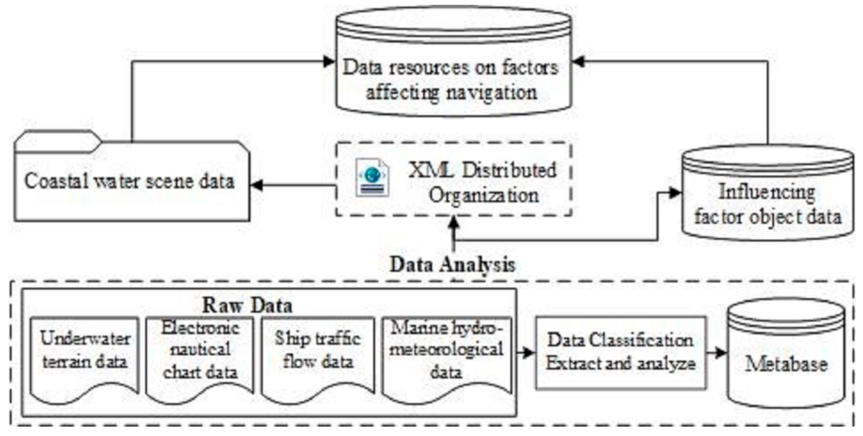
Due to the semantic independence and heterogeneity among data resources, as well as the differences in time, spatial dimensions, and storage methods, adopting a reasonable spatial data organization and storage method to construct a spatiotemporal dataset that affects navigation safety factors is the foundation for subsequent research. The application of XML schema organizes and manages the data sources, data types, information content, structure, and access methods of metadata in a unified manner, and stores them in a combination of files and databases to ensure the reuse of the model during data updates. This method constructs a spatiotemporal integrated data storage model with a unified spatial reference based on the hierarchical and correlated geographical distribution of entity elements, as shown in Figure 2.

2.2. Channel Boundary Extraction Based on Constrained Delaunay Triangle–Alpha-Shapes

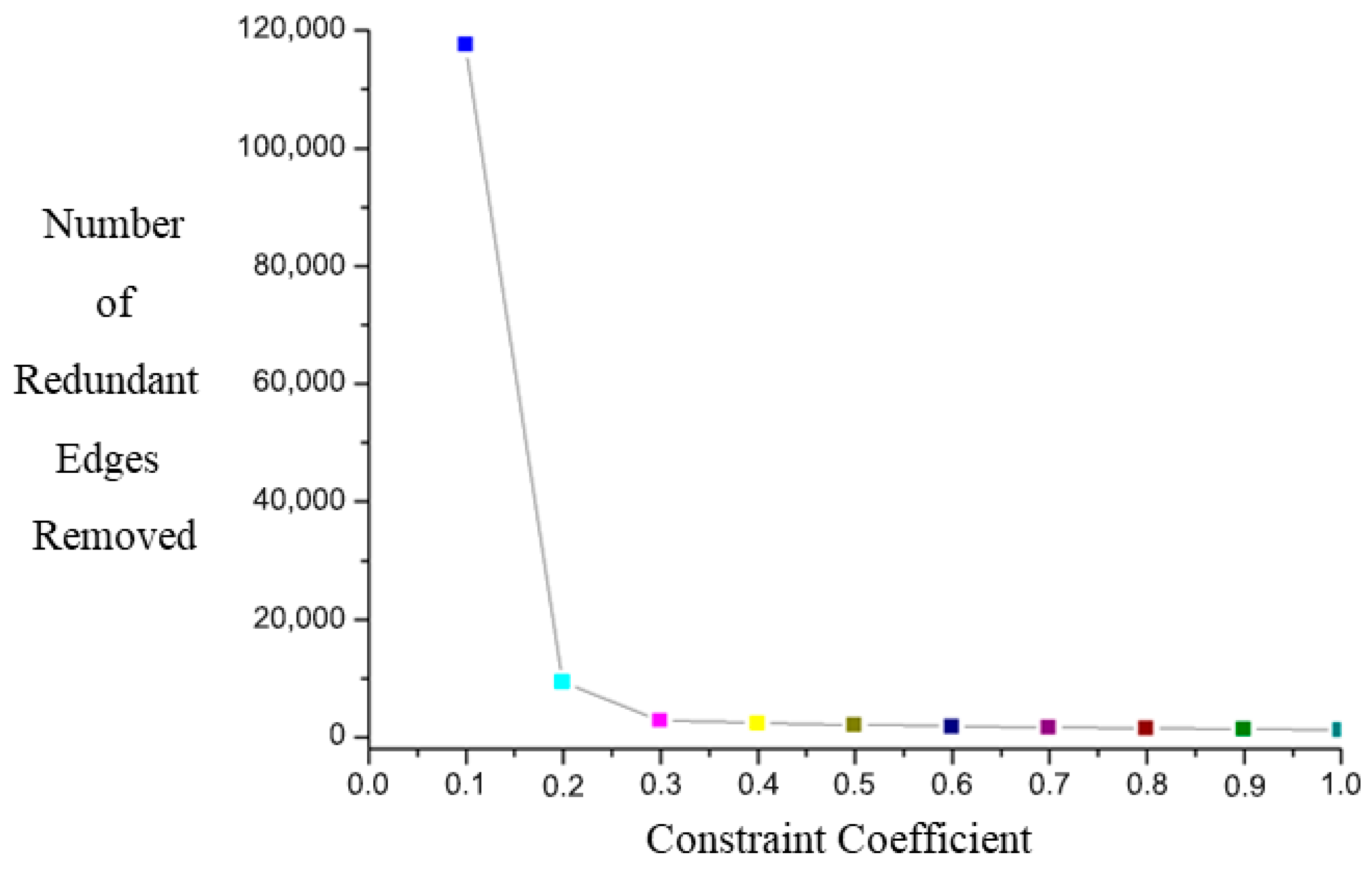
The Constrained Delaunay Triangle (CDT) is a special type of triangulation method that enhances Delaunay triangulation by incorporating the handling of constraint edges [36]. This method is widely applied in the boundary extraction of crowdsourced trajectory lines. When constructing a triangular mesh for waterways based on discrete points, the initial triangular mesh is generated by performing Delaunay triangulation on the input set of the bathymetric survey data points for the waterway. Subsequently, the triangular mesh is adjusted according to the input constraint edges to form triangles that are spatially adjacent and do not intersect with the constraint line segments. Redundant triangle edges are eliminated based on the statistical characteristics of the triangle side lengths. The Alpha-Shapes algorithm is a geometric shape algorithm that is used for boundary extraction. By controlling a rolling circle with a radius of α, it abstracts a contour shape from a discrete set of spatial points, providing a fundamental algorithm for the precise extraction of waterway boundaries.

The Alpha-Shapes algorithm can abstract the contour shape from a discrete set of spatial points by controlling a rolling circle with a radius of α [37]. For any pair of points ${\mathrm{P}}_1\left(x_1,{\mathrm{y}}_1\right)$ and ${\mathrm{P}}_2\left(x_2,{\mathrm{y}}_2\right)$, in the point set P and the center ${\mathrm{P}}_3\left(x_3,{\mathrm{y}}_3\right)$ of the circle passing through these two points with a radius of α, it is determined whether other points in the point set P are contained within the circle. The distances from the other points in the point set P to the center P₃ are calculated and compared with α. If the distances from all other points to the center P₃ are greater than α, then P₁ and P₂ are considered boundary points. The determination of the boundary points involves an iterative search process to check all possible pairs of point combinations. The calculation formula is as follows [37]:

$$\left\{\begin{array}{l}{{\displaystyle x}}_3={{\displaystyle x}}_1+{\displaystyle \frac{1}{2}}\left({{\displaystyle x}}_2-{{\displaystyle x}}_1\right)+H\left({{\displaystyle y}}_2-{{\displaystyle y}}_1\right)\\ {{\displaystyle y}}_3={{\displaystyle y}}_1+{\displaystyle \frac{1}{2}}\left({{\displaystyle y}}_2-{{\displaystyle y}}_1\right)+H\left({{\displaystyle x}}_2-{{\displaystyle x}}_1\right)\end{array}\right.$$

(1)

In Equation (1), H is a factor related to α and the distance between the two points. The calculation formula for H is as follows:

$$H=\sqrt{{\displaystyle \frac{a^2}{{(x_2-x_1)}^2+{(y_2-y_1)}^2}}-{({\displaystyle \frac{|x_2-x_1|}{2}})}^2}$$

(2)

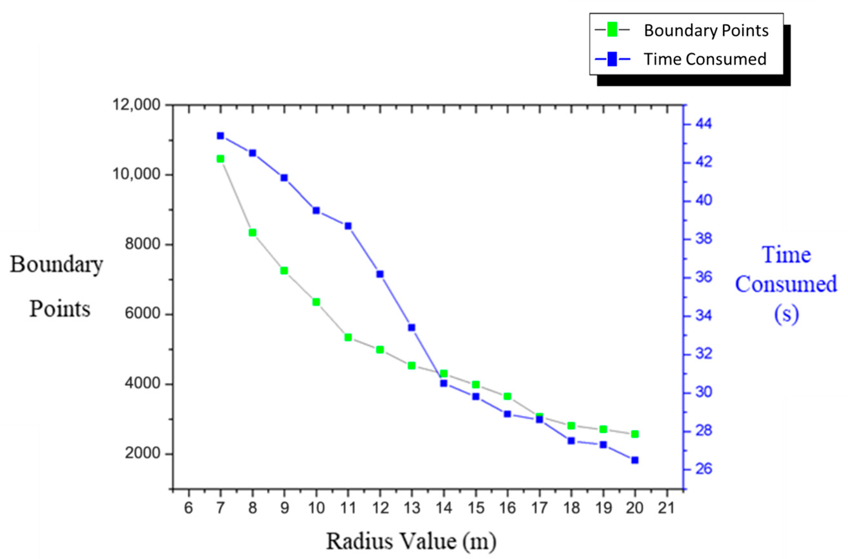
In Equation (2), H is adjusted according to the actual situation and is directly related to the distance from the point to the circle’s center and α. The choice of the radius α affects the result of the boundary extraction. A value that is too small can lead to discontinuities, making it impossible to form an effective boundary. A value that is too large will include non-boundary points, resulting in a boundary that does not accurately reflect the actual situation. An appropriate value can be used to effectively identify boundary points and form a waterway boundary line that reflects the actual situation. In the actual process of waterway boundary extraction, when the set circle radius α is sufficiently small, every point in the dataset can be considered a potential boundary point. By repeatedly adjusting the parameters and testing, gradually increasing the value of α, and performing rolling calculations on the boundary points until all point sets are covered and processed, the continuous rolling trajectory of the circle is ultimately used to accurately define the boundary of the dataset, thereby completing the effective extraction of the waterway boundary.

2.3. Extraction of Ship Navigation Boundaries Based on CDT–Voronoi

The ship navigation trajectory data in coastal waters exhibit uneven distribution characteristics. Taking the data for a container ship as an example, CDT combined with distance threshold adjustment is effectively used to eliminate redundant edges and extract the outer boundary. However, it is difficult to extract the inner boundary using the Alpha-Shapes algorithm. As an important branch of computational geometry, the Voronoi diagram leverages its nearest neighbor property to represent the spatial relationships among numerous discrete data points.

The edge of a ship trajectory point set, especially in areas where the density suddenly changes, can reflect the intensity and scope of ship navigation in coastal waters. The intensity of the point concentration is determined by the graphic density value. When the graphic density value is high, it indicates that the ship trajectory points in that area are densely distributed and that ship navigation activities are frequent. Conversely, a lower graphic density value suggests a sparse distribution of ship trajectory points and fewer ship navigation activities in that area. A higher numerical value indicates a denser ship trajectory, while a lower value suggests sparsity. The density ρ of the ship points is derived by calculating the reciprocal of the polygon’s area with the following formula [36]:

$$\rho ={\displaystyle \frac{1}{\frac{1}{2}|{\displaystyle \sum _{i=1}^{n-1}(x_i{y}_{i+1}-x_{i+1}{y}_i)+}(x_n{y}_1-x_1{y}_n)|}}$$

(3)

To further extract the inner boundary area of ship navigation, the density change rate index [36] is used. Based on the duality relationship between the Voronoi diagram and CDT, the vertices of the Delaunay triangles correspond to the densities of the ship points. The density change rate index is determined by calculating the difference or ratio between the densities of these points. The formula for calculating the density change rate index for each edge is as follows:

$$DCR{I}_{E_i}=\left\{\begin{array}{l}{\rho }_{il}/{\rho }_{ir},{\rho }_{il}\le {\rho }_{ir}\\ {\rho }_{ir}/{\rho }_{il},{\rho }_{il}>{\rho }_{ir}\end{array}\right.$$

(4)

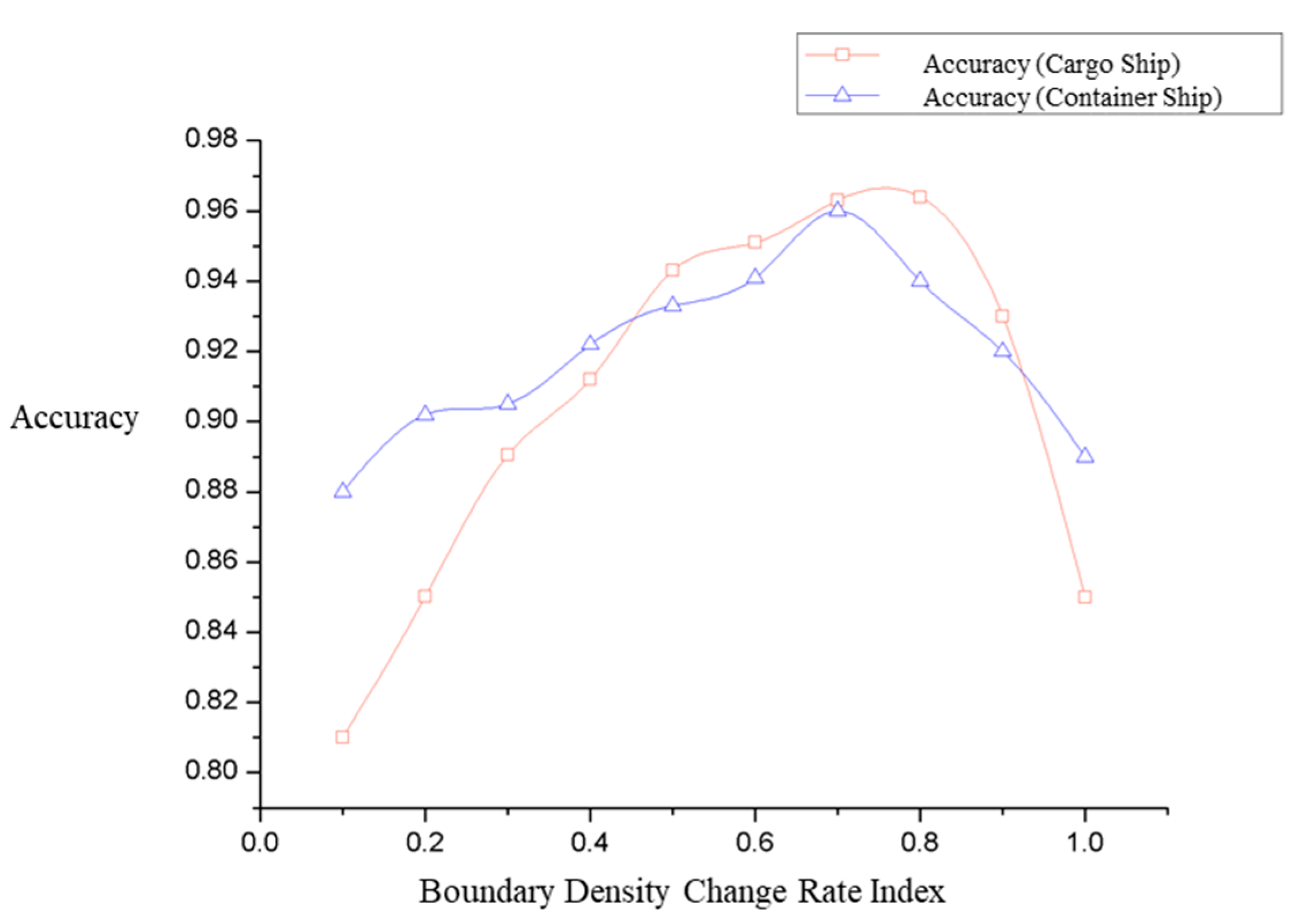
In Equation (4), ${\rho }_{il}$ and ${\rho }_{ir}$ represent the densities of the left and right vertices corresponding to the edge of the triangle, respectively. A smaller value of ${DCRI}_{Ei}$ indicates a greater density difference between the two points, which reflects a higher likelihood of being a ship navigation boundary. Conversely, a larger value suggests a higher likelihood of being a navigation area. By optimizing and adjusting the range of density thresholds and the density change rate index, the values of the edges of the Delaunay triangles can be obtained, and the internal boundary of the ship’s navigation trajectory can be extracted.

The data utilized in this section primarily consist of ship AIS data point sets, as well as data on navigation channels, anchorages, restricted areas, and navigational aids extracted from electronic nautical charts. By overlaying graphics derived from ship navigation boundaries with the electronic nautical chart data, an irregular grid was ultimately constructed.

2.4. Construction of Marine Hydro-Meteorological Data Fusion Grid

Marine hydro-meteorological information has multi-temporal data characteristics. The wind, wave, and current forecast data used are vector data based on regular cell grids. The grid range is set using the coordinates of the minimum bounding rectangle of the demonstration sea area, where each grid cell has a width and height of 0.01° in the longitude and latitude directions. The bilinear interpolation method for grid value assignment is used to establish an interpolation function based on two variables and linearly extend the function. Given the known values of four points, Q₁₁, Q₁₂, Q₂₁, and Q₂₂, the value of the function f(x) at point P is determined.

By uniformly dividing the grid, a regular geospatial grid for the marine environment is constructed. Based on grid calculations and value assignments, the vector graphics of the marine hydro-meteorological environment are formed on a grid basis. Data reclassification primarily involves reclassifying or reassigning pixel values in the raster data to generate a new raster dataset. Taking wind field data as an example, the magnitude of wind speed values serves as the primary basis for data reclassification. The classification method adopts equal intervals, dividing the data into 10 categories, where 1 and 10 represent low and high values, respectively. Pixel value merging calculations are performed according to the cell index values to obtain a reclassification map of the merged wind, wave, and current data. Based on the attribute values of the merged data, features with the same values are fused into a single feature. Additionally, the fused value field is written into the output feature class. Continuous lines are merged at common endpoints to generate multiple data features.

2.5. Construction of Unstructured Grid Fusion

Building upon the research methods mentioned earlier, we extracted the channel boundaries of coastal waters using electronic nautical charts and bathymetric data. Additionally, the actual navigation boundaries of different vessels in coastal waters were derived from Automatic Identification System (AIS) data. By fusing the channel boundaries with the navigation boundaries, we determined the overall boundaries of actual vessel navigation. Subsequently, the marine hydro-meteorological data were integrated into these overall boundaries, and data processing operations such as segmentation and merging were performed. A spatial overlay analysis was employed to superimpose grids formed with various influencing factors, including terrain, vessels, and the marine environment. Unstructured grids were thereby constructed for navigation in coastal waters.

Furthermore, considering the characteristics of different vessel types and the temporal features of marine data elements, the unstructured grids were generated on an hourly basis according to the navigation boundaries of the various vessel types. This provided a spatial unit grid map for subsequent evaluation and analysis of navigation safety.

3. Results

The fundamental concepts of quantitative evaluation and analysis are the determination of the evaluation set and the weights of evaluation indicators that affect navigation safety, the establishment of membership functions, and the construction of a fuzzy matrix. The fuzzy matrix is then operated upon with a weight vector to obtain quantitative comprehensive evaluation results. In this research, the fuzzy evaluation method is adopted to conduct quantitative evaluation and analysis, with the specific steps outlined as follows:

(1) Determination of the influencing factor set: A set $\mathrm{U}=\{u_1,u_2,\dots ,u_n\}$ is composed of various factors that influence navigation safety. The primary influencing factor set U is categorized into three subsets: natural condition factors (U₁), traffic condition factors (U₂), and marine hydro-meteorological condition factors (U₃). The secondary indicators are subsets of each primary influencing factor. Specifically, the natural condition factors (U₁) are further divided into submarine terrain (U₁₁), anchorage areas (U₁₂), channels (U₁₃), restricted areas (U₁₄), and water depths (U₁₅). The traffic condition factors (U₂) include traffic flow (U₂₁), vessel density (U₂₂), vessel speed (U₂₃), and navigation aids (U₂₄). The marine hydro-meteorological condition factors (U₃) include wind (U₃₁), waves (U₃₂), sea currents (U₃₃), tides (U₃₄), and sea fog (U₃₅). The primary and secondary indicators collectively form the influencing factor set, as shown in

Table 2. Evaluation indicators for factors affecting navigation safety.

Evaluation Area	Evaluation Factors	Subset of Evaluation Factors
Influencing factor set U	Natural condition factors U1	Submarine terrain U11
		Anchorage areas U12
		Channels U13
		Restricted areas U14
		Water depths U15
	Traffic condition factors U2	Traffic flow U21
		Vessel density U22
		Vessel speed U23
		Navigation aids U24
	Marine hydro-meteorological condition factors U3	Wind U31
		Waves U32
		Currents U33
		Tides U34
		Fog U35

.

(2) Determination of the evaluation factor set: The following are selected as evaluation factors: the terrain relief amplitude, anchoring density, channel width, area proportion, water depth value, traffic flow, vessel density, average vessel speed, quantity of navigation aids, average wind speed, average wave height, average flow velocity, variation range, and annual number of sea fog days. Each of these is analyzed to form the evaluation factor set $\mathrm{V}=\{v_1,v_2,\dots ,v_n\}$.

(3) Determination of membership functions: Based on the nature of the evaluation factors, triangular membership functions are chosen for numerical normalization within the interval [0, 1]. Through membership degree calculations, fuzzy sets are formed. For any evaluation factor within the evaluation set, there is a corresponding membership function $\mathrm{A}\left(\mathrm{x}\right)\in [0,1]$, where A(x) is referred to as the membership degree of x to the fuzzy set A.

(4) Construction of the fuzzy relation matrix: For each evaluation factor object $u_i$ and evaluation factor indicator $v_j$, there exists a fuzzy relationship $r_{ij}$ that represents the fuzzy degree of $u_i$ with respect to $v_j$. Fuzzy evaluations are conducted for each influencing factor to form the relation matrix R.

$$\mathrm{R}=\left[\begin{array}{l}{\mathrm{R}}_1\\ {\mathrm{R}}_2\\ ⋮\\ {\mathrm{R}}_{\mathrm{m}}\end{array}\right]=\left[\begin{array}{cccc}{\mathrm{r}}_{11}& {\mathrm{r}}_{12}& \dots & {\mathrm{r}}_{1n}\\ {\mathrm{r}}_{21}& {\mathrm{r}}_{22}& \dots & {\mathrm{r}}_{2n}\\ ⋮& ⋮& \ddots & ⋮\\ {\mathrm{r}}_{m1}& {\mathrm{r}}_{m2}& \dots & {\mathrm{r}}_{mn}\end{array}\right]$$

(5)

In Equation (5), m equals 14, and n equals 5.

(5) Determination of the weight vector: The Analytic Hierarchy Process was used in this research to determine the relative importance of various influencing factors in the evaluation of navigation safety in coastal waters. Firstly, the 1–9 scale method is used to determine the relative importance of two elements. The difference in importance between the two elements is represented by the numbers 1 to 9 and their reciprocal. The larger the scale value, the more important the former element is compared to the latter. Secondly, based on the relationship between influencing factors, the relative importance between each element in the same level is quantitatively represented, and the values are filled in to construct a judgment matrix U. Finally, the consistency of the judgment matrix is checked, and the consistency index (CI) and consistency ratio (CR) are calculated. The CI value reflects the degree of consistency of the judgment matrix. The smaller the CI value, the better the consistency of the judgment matrix; that is, the element relationships in the matrix are logically more reasonable.

In order to further determine whether the consistency of the judgment matrix is acceptable, the average random consistency index RI is introduced, and the consistency ratio CR, which is the ratio of CI to RI, is calculated. When CR is lower 0.1, the consistency of the judgment matrix is considered acceptable. Conversely, if CR is higher 0.1, the judgment matrix needs to be modified until the consistency requirement is met. We calculated the λmax of the judgment matrix to be 15.8296, with a matrix order of 14. The consistency of the 14 × 14 judgment matrix was quantitatively assessed using the Analytic Hierarchy Process (AHP) consistency metrics. The Consistency Index (CI) was calculated as

$$CI={\displaystyle \frac{\lambda max-n}{n-1}}={\displaystyle \frac{15.8296-14}{14-1}}=0.141$$

where λmax = 15.8296 denotes the principal eigenvalue obtained via Frobenius norm optimization, and n = 14 represents the matrix dimensionality.

The consistency ratio (CR) was then derived by normalizing CI against the 14th-order Random Index (RI₁₄ = 1.58):

$$CR={\displaystyle \frac{CI}{{RI}_{14}}}={\displaystyle \frac{0.141}{1.58}}=0.089$$

Since CR = 0.089 < 0.10, the matrix satisfies AHP’s consistency threshold. Calculate according to the above steps and use the sum product method to obtain the weight vector $\mathrm{W}=\{{\mathrm{w}}_1,{\mathrm{w}}_2,\dots ,{\mathrm{w}}_{\mathrm{n}}\}$, where ${\mathrm{w}}_{\mathrm{j}}$ represents the weight of the evaluation indicator ${\mathrm{v}}_{\mathrm{j}}$.

(6) Fuzzy operation: A fuzzy operation is performed on the fuzzy relation matrix and the weight vector to obtain the evaluation result B.

$$B=\overrightarrow{W}\times M=\left[b_1,b_2,b_3,\dots \dots \left.b_n\right]\right.$$

(6)

The $b_i$ term represents the comprehensive evaluation result of the evaluation object $u_i$, and it is calculated as follows:

$$b_i={\displaystyle \sum _{j=1}^n\stackrel{\rightharpoonup }{w_j}\times r_{ij}}$$

(7)

The performance of quantitative analysis using numerical values and the determination of the risk levels constitute the core concepts of the dynamic grid safety evaluation model for coastal waters. The evaluation values and membership degrees of each influencing factor are calculated sequentially, as shown in

Table 3. Calculation of evaluation factor quantization values and membership set.

No.	Evaluation Factor	Quantified Value	Membership Degree Set
1	Terrain relief amplitude	2.5	(0.25, 0.75, 0, 0, 0)
2	Anchoring density	0	(1, 0, 0, 0, 0)
3	Channel width	253	(0.47, 0.53, 0, 0, 0)
4	Area proportion	0	(1, 0, 0, 0, 0)
5	Water depth value	−18.2	(0, 0.18, 0.82, 0, 0)
6	Traffic flow	158	(0, 0, 0, 0.79, 0.21)
7	Vessel density	1.67	(0, 0, 0, 0.835, 0.165)
8	Average vessel speed	6.2	(0.4, 0.6, 0, 0, 0)
9	Number of navigation aids	36	(1, 0, 0, 0, 0)
10	Average wind speed	2.28	(0.14, 0.86, 0, 0, 0)
11	Average wave height	0.23	(1, 0, 0, 0, 0)
12	Average flow velocity	0.27	(1, 0, 0, 0, 0)
13	Variation range	0.54	(1, 0, 0, 0, 0)
14	Annual number of sea fog days	7	(0.4, 0.6, 0, 0, 0)

.

The specific calculation process for the evaluation results of the divided unstructured grid cells is as follows:

$$\begin{array}{c}B={\left[\begin{array}{l}\begin{array}{r}\hfill 0.065\end{array}\\ \begin{array}{r}\hfill 0.078\end{array}\\ \begin{array}{r}\hfill 0.075\end{array}\\ \begin{array}{r}\hfill 0.062\end{array}\\ \begin{array}{r}\hfill 0.074\end{array}\\ \begin{array}{r}\hfill 0.084\end{array}\\ \begin{array}{r}\hfill 0.082\end{array}\\ \begin{array}{r}\hfill 0.078\end{array}\\ \begin{array}{r}\hfill 0.087\end{array}\\ \begin{array}{r}\hfill 0.067\end{array}\\ \begin{array}{r}\hfill 0.074\end{array}\\ \begin{array}{r}\hfill 0.054\end{array}\\ \begin{array}{r}\hfill 0.057\end{array}\\ \begin{array}{r}\hfill 0.063\end{array}\end{array}\right]}^T\times \left[\begin{array}{ccccc}0.25& 0.75& 0& 0& 0\\ 1& 0& 0& 0& 0\\ 0.47& 0.53& 0& 0& 0\\ 1& 0& 0& 0& 0\\ 0& 0.18& 0.82& 0& 0\\ 0& 0& 0& 0.79& 0.21\\ 0& 0& 0& 0.835& 0.165\\ 0.4& 0.6& 0& 0& 0\\ 1& 0& 0& 0& 0\\ 0.14& 0.86& 0& 0& 0\\ 1& 0& 0& 0& 0\\ 1& 0& 0& 0& 0\\ 1& 0& 0& 0& 0\\ 0.4& 0.6& 0& 0& 0\end{array}\right]\\ =\left[\begin{array}{ccccc}0.529& 0.244& 0.061& 0.135& 0.031\end{array}\right]\end{array}$$

(8)

The numerical result was obtained by multiplying the fuzzy relation matrix and the weight vector for navigation safety in coastal waters. Based on the weighted calculation, the safety level was determined, and the safety evaluation result for the grid was derived. The evaluation result for matrix B was calculated as 0.529 × 1 + 0.244 × 2 + 0.061 × 3 + 0.135 × 4 + 0.031 × 5 = 1.895. This value was matched with the corresponding risk level grades [1, 2, 3, 4, 5] representing the low, relatively low, medium, relatively high, and high risk levels. Consequently, the risk level grade for this grid’s evaluation result is determined to be relatively low.

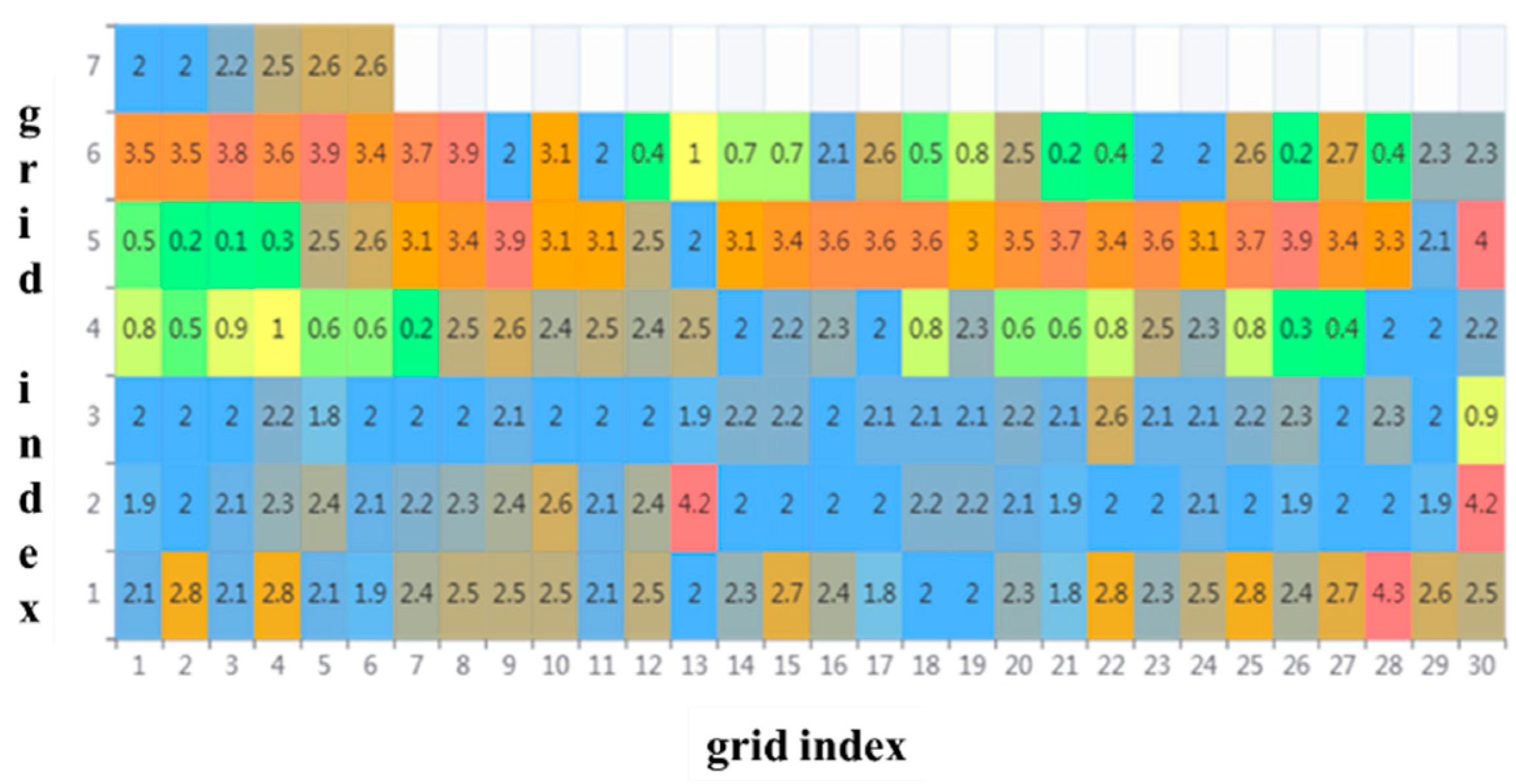
A 3 h period from 7:00 AM to 9:00 AM was selected as the time unit. The serial numbers of the unstructured grid cells were recorded. Figure 3 illustrates the calculation results for the evaluation calculations performed on the 186 divided unstructured grids using the fuzzy relation matrix and weight vector for navigation safety evaluation in coastal waters.

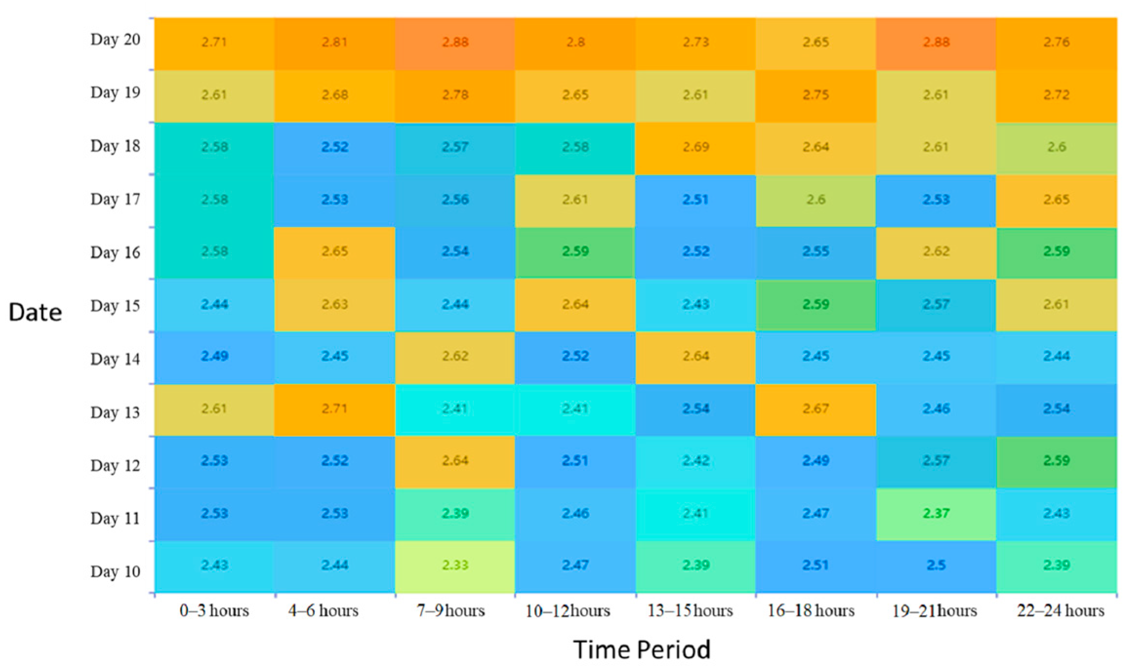
Similarly, by selecting data from ten days, with time series as the axis and 3 h as the unit, the evaluation result values of a grid at 88 moments in the time series are calculated, as shown in Figure 4.

According to statistics, the grid was assessed as medium risk at all 88 time points during this period, which does not affect navigation safety. However, the evaluation results vary at different times, mainly due to the influence of environmental factors such as ocean winds, waves, currents, and tidal changes.

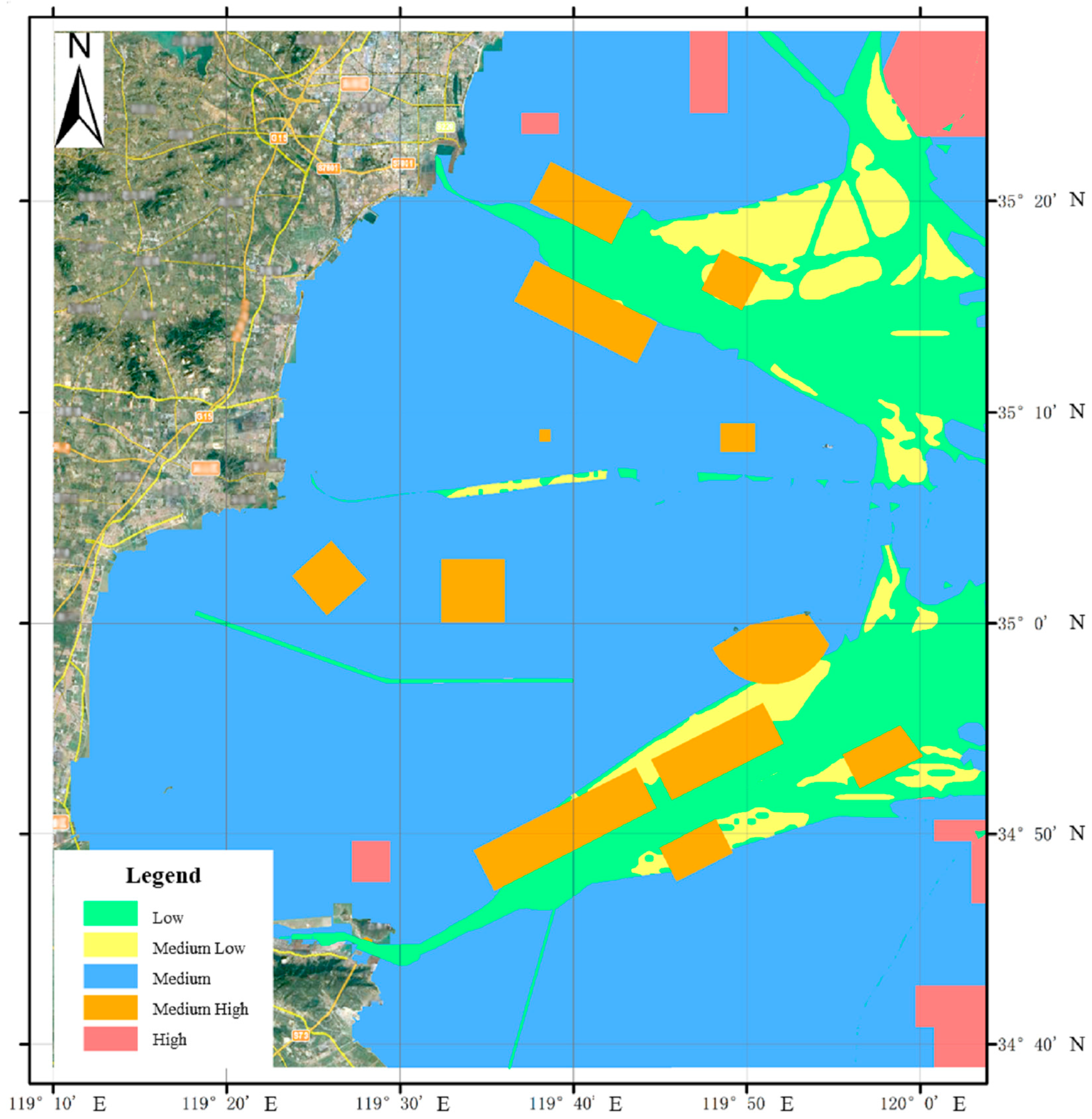
The main purpose of determining ship navigation safety in coastal waters is to identify and analyze potential safety risks during the navigation process, while risk level is determined by identifying risk factors during the navigation process, evaluating their possible consequences and probability of occurrence. The risk level for each grid was categorized into five grades: low, relatively low, medium, relatively high, and high. Based on these risk level grades, a color classification system was established for the grids, resulting in a five-color thematic map depicting the geospatial risks of the grid cells in the sea area. This map provided graphical support for navigation safety, as illustrated in Figure 5. After statistical analysis, out of the 186 unstructured grid cells constructed, 4 were classified as high-risk, primarily in areas with restricted navigation. There were 28 grid cells classified as relatively high-risk, mainly in anchorage areas and similar regions. The majority, 116 grid cells, were classified as medium-risk, and these essentially covered the entire coastal water area. The remaining 38 grid cells were classified as low- or relatively low-risk, and were predominantly in channels and vessel-operable waters.

4. Discussion and Analysis

It is necessary to adjust algorithm parameters in the extraction of channel and ship navigation boundaries. Based on experimental data from a demonstration sea area, in this research, result analysis and method evaluation were conducted by adjusting the values of the parameter indicators.

4.1. Analysis of Channel Boundary Extraction Method

During the process of channel boundary extraction, the key factors were the distance threshold for constraining the length of the triangle edges (the value of the constraint parameter α) and the selection of the circumradius for the Alpha-Shapes algorithm. By constructing a triangular network of the channel based on discrete points and adjusting the value of the constraint parameter, the distance threshold for the edge lengths was calculated.

Table 4. Statistical data for the side lengths of the channel triangulation network.

No.	Constraint Parameter	Threshold of Edge Length for Constrained Triangulation Network (m)	Average Edge Length of Constrained Triangulation Network (m)	Standard Deviation of Edge Length for Constrained Triangulation Network (m)
1	0.1	12.249	9.19	30.59
2	0.2	15.308	9.19	30.59
3	0.3	18.367	9.19	30.59
4	0.4	21.426	9.19	30.59
5	0.5	24.485	9.19	30.59
6	0.6	27.544	9.19	30.59
7	0.7	30.603	9.19	30.59
8	0.8	33.662	9.19	30.59
9	0.9	36.721	9.19	30.59
10	1.0	39.78	9.19	30.59

summarizes the statistical data for the channel triangular network that were determined through comparative analysis.

The value range of the constraint parameter α was [0, 1]. By adjusting the value of this parameter, the distance threshold for the edge lengths was calculated. Through comparative analysis after the removal of the redundant edges, as illustrated in Figure 6, it was determined that when α had a smaller value, the redundant edges that were removed encompassed the entire channel triangular network. Conversely, when α had a larger value, not all of the redundant edges could be removed.

Outer boundary channel extraction mainly consists of adjusting the circumradius parameter of the Alpha-Shapes algorithm. Based on the extracted channel boundary points, the value of the parameter radius α was adjusted to determine the optimal outer boundary of the channel. Figure 7 illustrates the variation in the parameter radius α from small to large values, which was determined by recording the number of points and the time consumption for the extraction of the outer boundary of the channel. It can be observed from the figure that when the radius α was set to 14, the number of extracted outer boundary points was 4299, and the time taken was 30.5 s. As the radius value increased, there was only a slight change in the number of extracted points and the time consumption. Using a comparison with the actual outer boundary of the channel, it was found that the data used in this research achieved the best fit when the radius α was set to 14, with relatively high algorithm computational efficiency.

4.2. Analysis of Ship Navigation Boundary Extraction Method

To study navigation safety assessment in coastal waters, in this research, container ships and cargo ships were taken as examples from which to extract ship navigation boundaries. Based on the Voronoi diagram, the regional density value (density of ship points ρ) was calculated by computing the area of constructed graphical regions. The density change rate index (${\mathrm{D}\mathrm{C}\mathrm{R}\mathrm{I}}_{Ei}$) for each edge was then calculated using the values of the Thiessen polygon edges. By simultaneously analyzing these two values, the value ranges were gradually determined, and data boundary processing was conducted for the Thiessen polygons. According to the generated data statistics, the regional density value range for the container ships was (0, 29.38], and for cargo ships, the range was (0, 29.61]. The ship’s AIS data were rasterized to form polygons. Based on the method proposed in this paper, the navigation boundary areas were extracted. A spatial overlay analysis was performed for the extracted navigation boundary areas and the polygonal regions formed by the ship point sets to represent the accuracy of the algorithm. The formula for calculating the accuracy is as follows:

$$precision=\left\{\begin{array}{l}regio{n}_{ext}/regio{n}_{all} regio{n}_{ext}\le regio{n}_{all}\\ regio{n}_{all}/regio{n}_{ext} regio{n}_{ext}>regio{n}_{all}\end{array}\right.$$

(9)

In Equation (9), $regio{n}_{ext}$ represents the extracted navigation boundary area, $regio{n}_{all}$ represents the polygonal area formed by the ship point set, and precision signifies the accuracy. An accuracy value close to 1 would indicate that the extracted boundary was relatively complete. Through comparison with the actual ship positions, it was found that the accuracy was high when the regional density value range for the container ships was [0.6, 29.38], and for cargo ships, the range was [0.6, 29.61]. Further comparative analysis of the density values revealed that the accuracy was the highest when the regional density for container ships was greater than 0.63, and for cargo ships, the accuracy was the highest when the regional density was greater than 0.65, as illustrated in Figure 8.

Building upon the regional density value ranges, we continuously adjusted the values of the boundary density change rate index (${\mathrm{D}\mathrm{C}\mathrm{R}\mathrm{I}}_{Ei}$). When the ${\mathrm{D}\mathrm{C}\mathrm{R}\mathrm{I}}_{Ei}$ for the container ships was set to 0.71 and that for cargo ships was set to 0.77, the extracted ship navigation boundaries aligned well. Consequently, we derived the navigation boundaries for different types of ships, as depicted in Figure 9.

4.3. Comparative Analysis of Structured Grid and Unstructured Grid

Referring to the comparative experiment of structured and unstructured ocean forecasting models constructed by Trotta, F. et al. [38], we divided the coastal waters into regular grids with accuracies of 36″ × 36″, 20″ × 20″, 15″ × 15″, 10″ × 10″, and 5″ × 5″. The grids that intersect with the coastline have been removed, resulting in the construction of a standardized grid for the nearshore waters. According to the evaluation method in Section 3, a risk analysis was conducted on the divided regular grid, and the number of risk grids was calculated for each of five types, as shown in

Table 5. Statistics of risk areas divided into different types of grids.

Grid Type	Grid Accuracy	Grids Count	High-Risk Grid Count	Medium—High-Risk Grid Count	Medium-Risk Grid Count	Medium—Low-Risk Grid Count	Low-Risk Grid Count
Structured grid	36″ × 36″	11,976	269	1902	7521	708	1576
	20″ × 20″	38,273	821	5861	23,871	2205	5515
	15″ × 15″	67,895	1325	11,220	40,346	3816	11,188
	10″ × 10″	152,435	3078	22,047	98,066	8816	20,428
	5″ × 5″	608,423	11,085	79,590	329,446	31,953	156,349
Unstructured grid	-	186	4	28	116	11	27

.

By comparing and analyzing the time consumption for generating different types of grids, risk assessment, and total time consumption, it can be concluded that the time consumption for generating regular grids with different accuracies is not significantly different, while the time consumption for generating irregular grids is relatively high, mainly in data fusion. In terms of risk assessment, the number of grids is positively correlated with computation time, and the more grids are divided, the longer the time consumption. Overall, the total time consumption is related to the accuracy of grid division, mainly due to the time required for conducting risk assessment and data calculation for each grid, as shown in Figure 10.

In general, within the framework of regular grid partitioning, a finer grid division leads to higher accuracy in evaluating risk areas, albeit at the cost of significantly increased computational time. Therefore, the unstructured grid partitioning method proposed in this paper not only ensures time efficiency but also effectively reflects the distribution of risk areas in coastal waters, demonstrating marked advantages over regular grids in dynamic data computation scenarios.

5. Conclusions

The risk profile of coastal waters exhibits functional characteristics in both time and space, evolving over time and varying with spatial location. The unstructured grid risk graphics for coastal waters incorporate spatiotemporal dimensionality, offering technical support and safety assurance for navigation. The conclusions of this study are as follows:

(1) A multi-factor fused dynamic irregular grid partitioning method for maritime areas was proposed. This method accurately extracted channel boundaries using the CDT–Alpha-Shapes approach and precisely identified ship navigation areas through the CDT–Voronoi method. By integrating grids based on oceanic wind, wave, and current data, unstructured grids with temporal characteristics were constructed, enabling dynamic reflection and fine partitioning of the maritime navigation environment. This approach not only enhanced the precision and flexibility of maritime grid partitioning, but also comprehensively considered the multifactorial impacts on navigation safety. This allowed for dynamic adjustments in grid partitioning in response to changes in channel conditions, ship traffic flow, and the marine environment, providing a more scientific and refined technical means for evaluating and managing navigation safety in coastal waters.

(2) A navigation safety assessment model and a quantitative analysis method for coastal waters were proposed. This method systematically constructed an influencing factor set and an evaluation factor set for navigation safety, considering various influencing factors. The quantitative criteria for each type of evaluation indicator were established, enabling the precise description of multidimensional factors that influence navigation safety. Based on this, a fuzzy relation matrix was constructed by solving the membership degree vector through membership functions, and a weight vector was established using the sum–product method. Quantitative analysis and evaluation of navigation safety for irregular grids in coastal waters were conducted, safety levels were determined, and risk thematic maps were constructed, enhancing the scientificity and accuracy of navigation safety assessments.

In summary, the accuracy and timeliness of risk assessments were improved in graphics technology for coastal water unstructured grid risk; this was achieved by integrating spatiotemporal dimensionality and enabling the dynamic assessment, calculation, and visual display of risk factors, while solid technical support and safety assurance were provided for navigation. With continuous technological advancements and the expansion of application scenarios, this technology will play an increasingly vital role in the future in ensuring maritime traffic safety and promoting sustainable development in coastal waters.

However, there are still some issues and directions worth further exploration, mainly relating to the following points:

(1) In terms of constructing dynamic irregular grids, the data standards for different sea areas are not unified. In the process of using the method proposed in this paper to extract channel boundaries and ship navigation boundaries, parameter adjustments are still needed to obtain the most suitable calculation results through continuous debugging.

(2) In terms of risk assessment for maritime grid security, more influencing factors can be incorporated into the model based on actual conditions. It is necessary to construct and calculate the influencing factor set, evaluation factor set, fuzzy relationship matrix, and weight vector. This article still needs further improvement in terms of expansion.