Article

Probabilistic Noise Detection and Weighted Non-Negative Matrix Factorization-Based Noise Reduction Methods for Snapping Shrimp Noise

Department of Information and Communication Engineering, Changwon National University, Changwon-si 51140, Republic of Korea
*
Authors to whom correspondence should be addressed.
J. Mar. Sci. Eng. 2025, 13(1), 96; https://doi.org/10.3390/jmse13010096
Submission received: 5 December 2024 / Revised: 30 December 2024 / Accepted: 4 January 2025 / Published: 7 January 2025
(This article belongs to the Section Ocean Engineering)

Abstract

:
Snapping Shrimps (SSs) live in warm marine areas. Snapping Shrimps Noise (SSN), loud sounds generated by these underwater creatures, serves as a major source of in performance degradation by decreasing the Signal-to-Noise Ratio (SNR) for underwater acoustic communication and target detection. Thus, we propose a unified solution for SSN detection and reduction in this paper. First, Signal Presence Probability (SPP) is calculated for SSN detection, and then the SPP is provided to Non-negative Matrix Factorization (NMF) as a weight for SSN reduction. In the proposed method, SPP acts as a key factor for SSN detection and reduction. To verify the effectiveness of the proposed method, the SAVEX-15 dataset, real ocean data containing SSN, is used. As a result of SSN detection, it was confirmed that SPP presented the highest performance in the Receiver Operating Characteristics curve, and we achieved 0.014 higher Area Under the Curve compared to competing methods. In addition, Continuous Wave and Linear Frequency Modulation signals were set as target signals and combined with the SAVEX-15 data for evaluation of noise reduction performance. As a result, the performance of the SPP-weighted NMF (WNMF) presented at least 2 dB higher SNR and SDR while maintaining less LSD compared to the Optimally Modified Log Spectral Amplitude estimator and NMF.

1. Introduction

A snapping shrimp is a representative marine creature that lives within ±40° latitude [1,2,3]. Snapping shrimps frequently generate impulsive shock waves with a large claw when they protect themselves from natural enemies or engage in feeding activities [4]. This shock wave produces a high acoustic sound source level amounting to approximately 190 dB in an extremely short period of time [5]. The transient sound occurs multiple times within 10 ms, and the frequency response of the sound spans from 60 Hz to 250 kHz [6]. Thus, the sound of snapping shrimp is one of the major noise sources in underwater communication and underwater target detection areas [7,8,9,10,11,12].
Studies to detect the snapping shrimp noise (SSN) have been conducted [13,14,15]. As in previous studies of this paper, Park and Hong [13] detected the SSN interval by applying a Cell Average CFAR detector based on Linear Prediction (LP) analysis using the Shallow-water Acoustic Variability Experiment-2015 (SAVEX-15) dataset [14]. Subsequently, Park and Hong proposed an SSN detection method based on the Likelihood Ratio (LR) derived from statistical modeling of the LP residual signal [15]. The performance of SSN is improved from the method using the LP residual signal in [13] to the LRs derived by statistical modeling of the LP residual signal in [15]. However, SSN detection performance is not sufficient, and an SSN reduction method is required.
Thus, in this paper, we propose a unified solution for detecting and reducing SSNs based on the study in [15]. For SSN detection, the LR obtained in [15] is combined with a priori Signal Absence Probability (SAP) estimator to convert it into a Signal Presence Probability (SPP). For evaluation, the Receiver Operating Characteristics (ROC) curve [16] and Area Under the Curve (AUC) were compared with the previous works in [13,15]. Subsequently, the SPP is provided to Weighted Non-negative Matrix Factorization (WNMF) [17] and works as a weight for SSN reduction because SPP inherently bounds between 0 and 1. In order to verify the performance of SSN reduction, SSN is synthesized with a Continuous Wave (CW) and a Linear Frequency Modulation (LFM) as target signals at various Signal-to-Noise Ratio (SNR), respectively. The proposed SPP-WNMF is compared with the basic Non-negative Matrix Factorization (NMF) without weighting [18,19,20] and the Optimally Modified Log Spectral Amplitude (OM-LSA) estimator-based transient noise removal method [21,22] in the aspects of SNR, Signal-to-Distortion Ratio (SDR) [23] and Log Spectral Distance (LSD) [24]. In brief, the novelty of the proposed approach is summarized as follows:
  • SPP is calculated for SSN detection, and the detection results are analyzed;
  • NMF weighted by the SPP is proposed to reduce SSN effectively;
  • The proposed SSN detection and reduction methods are integrated as a unified solution.
This paper is organized as follows. In Section 2, we explain the background techniques related to this study. In Section 3, we explain the proposed methods in detail. After that, the experimental environment and results are presented in Section 4. Finally, conclusions will be given in Section 5.

2. Related Works

In previous works of SSN interval detection, methods using LP analysis and an LR derived by statistical modeling are studied in [13,15], respectively. The signal model of a hydrophone input y ( n ) can be denoted as the sum of the SSN s ( n ) and background noise v ( n ) , y n = s n + v ( n ) , where n refers to the sample index.

2.1. SSN Detection

2.1.1. LP Analysis

LP analysis [25] is a technique for predicting a current sample value by the weighted sum of previous sample values. The estimated current sample value by using LP analysis can be denoted as follows:
y ~ n = i = 1 c y n i q i ,
where q i represents the c -order linear coefficient, meaning the past sample index used for prediction. Subsequently, the LP residual signal e ( n ) which means estimation error can be defined as e n = y n y ~ ( n ) , and it has been reported that e ( n ) of the interval where SSN is present becomes large due to the impulsive characteristics [13].

2.1.2. Statistical Model Based LR

In [15], the LP residual signal e ( n ) obtained through the LP analysis in [13] is defined as the sum of the residual signals of SSN e s ( n ) and background noise e v n , respectively, e n = e s n + e v ( n ) . Based on this approach, hypotheses H 0 and H 1 corresponding to LP residual signals e s ( n ) and e v n of the e ( n ) , respectively, can be defined as follows:
  H 0 : E m , k = E v m , k , H 1 : E m , k = E s m , k + E v m , k ,
where E m ,   k , E s m ,   k , and E v m ,   k mean spectra of the k -th frequency bin of the m-th frame of e n , e s ( n ) , and e v n , respectively. LRs of representative three distributions (Gaussian, Laplace, Gamma) in statistical analysis [26] and the Goodness-Of-Fit test is performed to find the best fit of the histograms of H 0 and H 1 .
LP residual-based SSN detection was first proposed in [13], and LR based on statistical modeling of the LP residual improved the SSN detection performance. However, SSN detection performance is still insufficient, and the two SSN detection methods have limitations that are inappropriate to use directly as weights for SSN noise reduction because the dynamic range is not bound from 0 to 1.

2.2. NMF-Based Source Separation Techniques

NMF [18,19,20] is a method that approximates an input non-negative matrix as the product of two non-negative matrices. In general, NMF can be expressed as,
V W H ,
where V represents the t × u input matrix, W is the t × r basis matrix, and H is the r × u weight matrix. Additionally, the condition r t + u < t u should be satisfied. To obtain matrices W and H , two objective functions are commonly used: minimizing the Euclidean distance function and minimizing the Kull-back Leibler divergence. Since W and H are not convex, the multiplicative update rule is employed.
To separate sources using NMF, the spectrogram of the input signal is employed, and a supervised scenario is generally assumed. Consequently, the basis matrix W for each source is precomputed during the training phase and used to obtain estimated values for each source in the separation process. Assuming that the basis matrix for the target signal is W A and the basis matrix for the noise signal is W B , the combined matrix W t r a i n can be represented as W t r a i n = [ W A : W B ] . Thus, (3) can be denoted by using the basis matrix W t r a i n as,
V W t r a i n H = W A : W B H .
Next, fix the previously obtained W A and W B during the test phase and update the H A and H B matrices. Then, estimates of the target signal and the noise can be expressed as,
A e s t = W A H A , B e s t = W B H B ,
respectively.
In addition, Virtanen proposed a WNMF in [17], which introduces a weight matrix G to NMF. Applying weights to each of the input matrix V provides flexibility to highlight and mitigate certain elements in the reconstruction process, which ultimately improves the quality of the separation. However, it is important to select an appropriate weight matrix because the weight matrix has a significant impact on the separation performance. For example, if the strength of the weight matrix is too strong, it may converge in the wrong direction, and if the strength is too weak, the information may not be fully used. From the perspective of source separation, if the characteristics of the sources to be separated are known in advance, this information can be utilized to improve the separation performance [27]. The WNMF is denoted as,
G V G W H ,
where stands for the Hadamard product, and it is equivalent to NMF if components of G are 1.

3. Proposed Approach

In this paper, we propose a unified framework for SSN detection and reduction: SPP-WNMF. The proposed SPP-WNMF is composed of two parts: SPP calculation for SSN detection and WNMF for SSN reduction. In the proposed method, SPP works as a key factor. The entire block diagram of the proposed method is illustrated in Figure 1.

3.1. SPP Calculation for SSN Detection

In [15], the statistical distribution of the LP residual signal of SSN was examined. Through the statistical modeling, LRs of the Gaussian, Laplace, and Gamma distribution, denoted as,
  Λ G E m , k = 1 1 + ζ ( m , k ) · e x p γ m , k ζ m , k 1 + ζ m , k ,
Λ L E m , k = 1 1 + ζ m , k · e x p 2 E R m , k + E I m , k · λ v m , k + λ s m , k λ v m , k λ v m , k + λ s m , k λ v m , k ,
and
Λ A E m , k = 1 1 + ζ ( m , k ) · e x p { 2 3 ( | E R m , k | + | E I m , k | ) · ( λ v m , k + λ s m , k λ v ( m , k ) λ v m , k + λ s m , k λ v ( m , k ) ) }
respectively, were obtained to detect intervals of SSN. Specifically, λ v ( m , k ) and λ s ( m , k ) are the variances of E v ( m , k ) and E s ( m , k ) , respectively, and E R ( m , k ) and E I ( m , k ) are the real and imaginary parts of E ( m , k ) , respectively. In addition, ζ ( m , k ) represents a priori SNR and γ ( m , k ) denotes a posteriori SNR. Accordingly, by Bayes’ theorem, the conditional probabilities of signal presence based on these LRs can be derived as follows:
p m , k = P H 1 m , k E m , k = 1 1 + e x p log q m , k + log 1 Λ m , k
where q m , k = P ( H 0 m , k ) represents the a priori SAP. Furthermore, we can obtain three types of SPPs, i.e., p G ( m , k ) , p L ( m , k ) , and p A ( m , k ) , depending on the distribution. It is worth noting that we can improve the detection performance simply by converting LR to SPP; however, more importantly, SPP can be used as a weight for SSN reduction because it is bound between 0 and 1 inherently.

3.2. SSN Reduction Using WNMF

For the purpose of noise reduction, SSN is the noise source, and CW and LFM are generally used for the Signal Of Interest (SOI) in underwater target detection or communication. The SSN reduction process is largely divided into two parts: training and testing. At first, the basis matrix W t r a i n are trained. In this case, the basis matrix in (4) can be represented as follows:
V W t r a i n H = W S O I : W S S N H ,
where W S O I is the basis matrix of the SOI trained through NMF and W S S N is the basis matrix trained through WNMF, applying
G S S N = p m ,   k , m = 1 , , M , k = 1 , ,   K ,
where M and K are the number of frames and frequency bins, respectively. In the training stage, (12) is imposed on W S S N H S S N as a weight for SSN.
In the test, we can obtain the estimate of the target signal and SSN by using the trained basis matrix as follows:
S O I e s t = W S O I H S O I , S S N e s t = W S S N H S S N .

4. Experiments

4.1. Experimental Environment

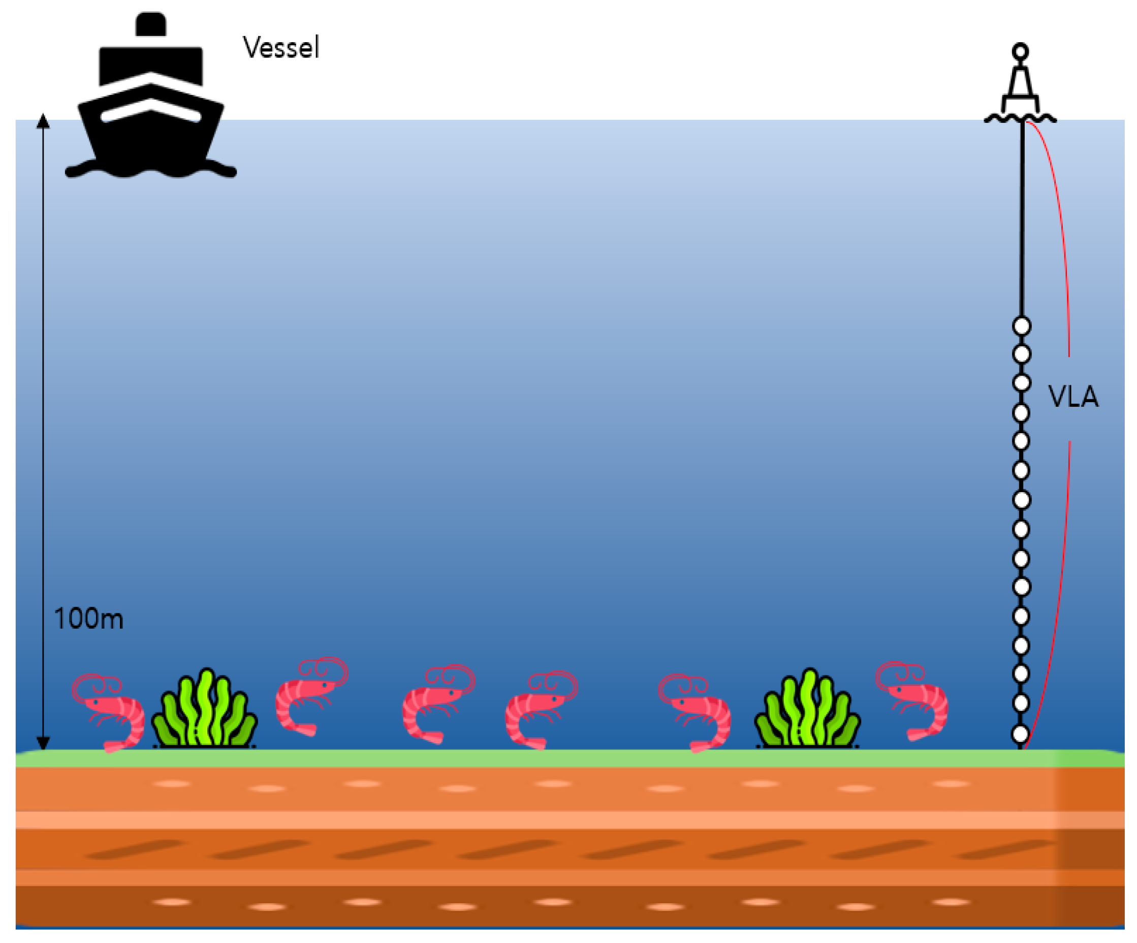
To evaluate the performance of the proposed method, we utilized the SAVEX-15 dataset collected in the real ocean environment where numerous SSs live. This dataset was collected in the region of 32°30′ N 126°05′ E–32°35′ N 126°12′ E, with 16 hydrophones evenly spaced on a Vertical Line Array (VLA) [14]. The SAVEX-15 dataset collection environment is illustrated in Figure 2.
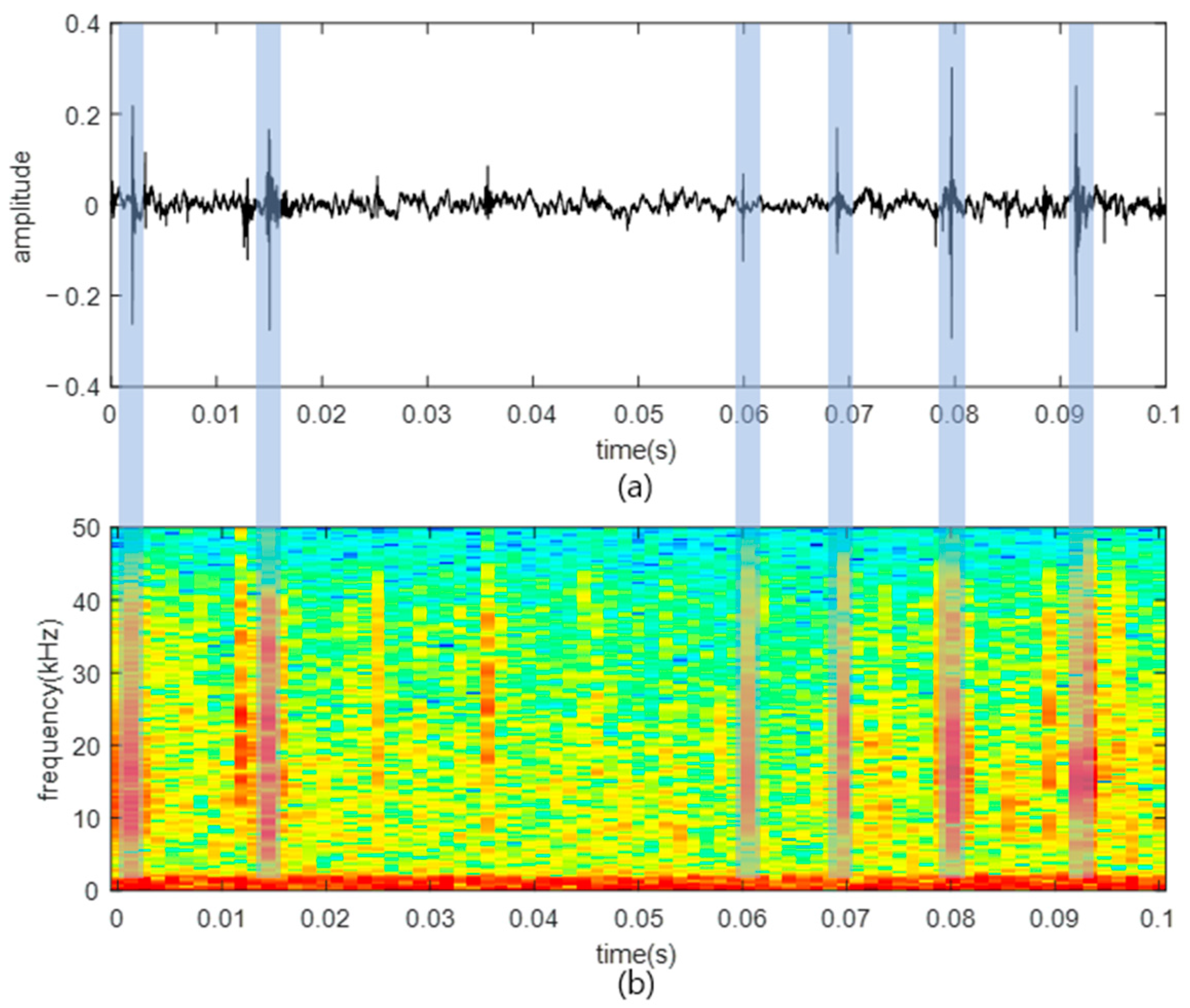
A part of the hydrophone input in the SAVEX-15 dataset is described in Figure 3. Several SSNs are observed in a 10 ms-long input signal. The characteristics of SSNs are highly transient in a time series and are spectrally flat with high energy in a short time in the spectrogram.
The experiments conducted in this paper can be broadly divided into two main categories: SSN detection and reduction.
First, we focused on detecting SSN as the target signal. For the validation of LR and SPP performance, LRs were computed under the same conditions as in [15], and labels of SSN intervals in the 100 s-long input data were manually marked.
Second, we reduced SSN in a dataset of mixed SSN by combining CW and LFM as target signals. To construct a noisy database, 10 s-long data in the SAVEX-15 dataset, excluding the data used for detecting SSN intervals, was extracted. Subsequently, CW and LFM signals were synthesized for 2 s to achieve target SNRs of −10, −5, 0, 5, and 10 dB. The frequency of the CW signal was fixed at 14 kHz, and the initial and end frequencies of the LFM signal were randomly selected between 7 and 8 kHz and between 10 and 12 kHz, respectively. Figure 4 represents the synthesized spectrogram of CW and LFM, respectively, when the synthesis SNR is 0.
Next, to train the basis matrices of CW and LFM, fifty 2 s-long noisy input signals were generated and synthesized at SNR, randomly selected between −10 and 10 for each signal. In the case of CW, the signal was placed in the form of steps so that all bands could be included, and in the case of LFM, the band of the signal was randomly selected. Furthermore, the sizes of the basis matrices for the SSN were set to 128, and SOIs (CW, LFM) were set to 32 and 64.
To evaluate the performance of SSN reduction, we compared conventional methods with the NMF method in [20] and a method using OM-LSA for transient noise reduction [22]. In [22], Minima Controlled Recursive Averaging (MCRA) [28] is modified to estimate the transient noise Power Spectral Density (PSD) for noise estimation. The obtained noise PSD is then applied to the OM-LSA filter to effectively remove the transient noise. In our experiments, the smoothing parameter for PSD tracking through MCRA was set to 0.1 for rapid adaptation.

4.2. Experimental Result

4.2.1. SSN Interval Detection

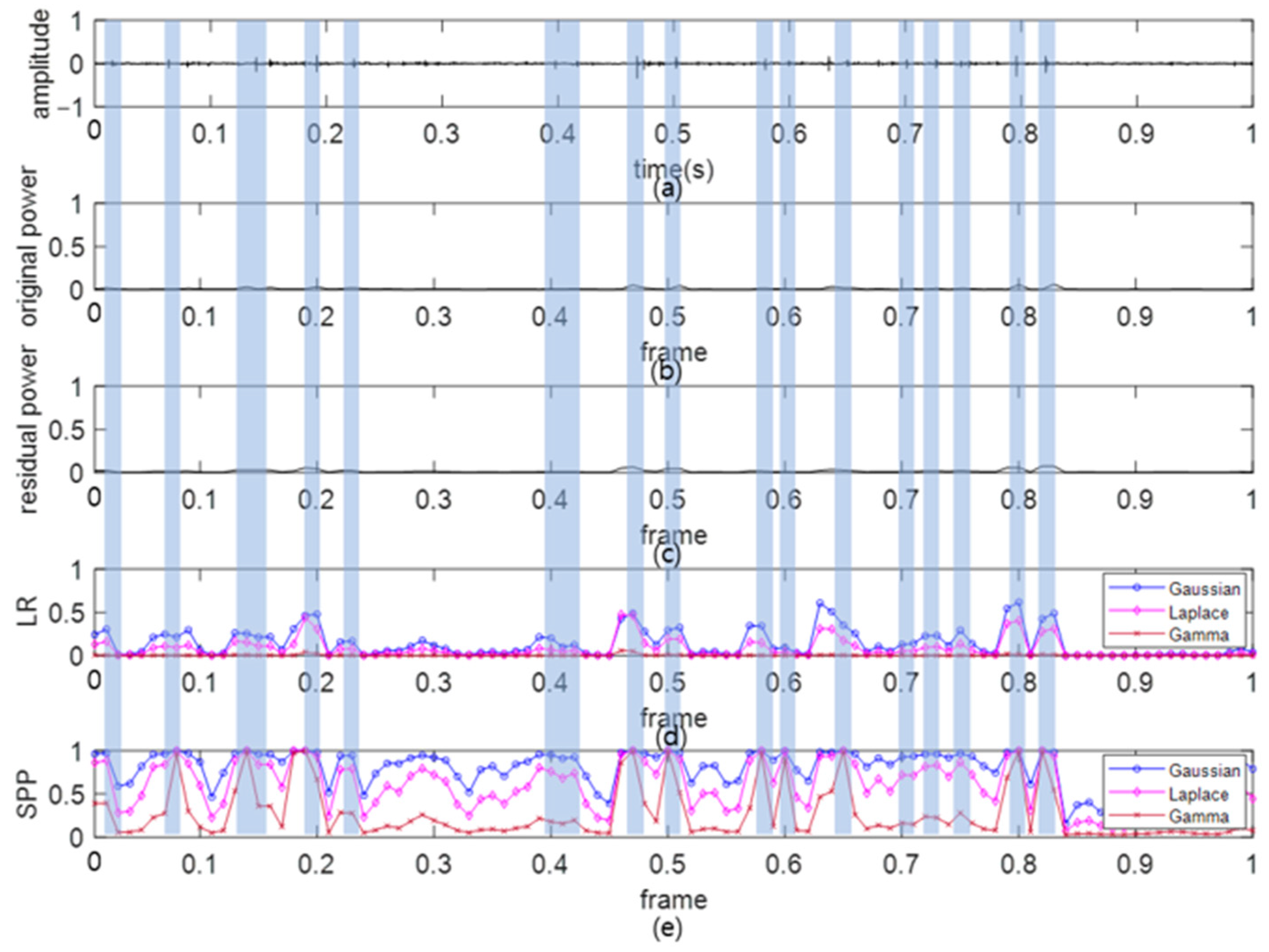
In order to examine the discriminative characteristics of the proposed methods visually, we compared the contours of input signal power, LP residual, LRs, and SPPs in Figure 5. All the features are normalized to be bound between 0 and 1. Several blue vertical bars denote SSN intervals. Overall, the peaks of SPPs in the SSN intervals are more prominent than the other competing contours.
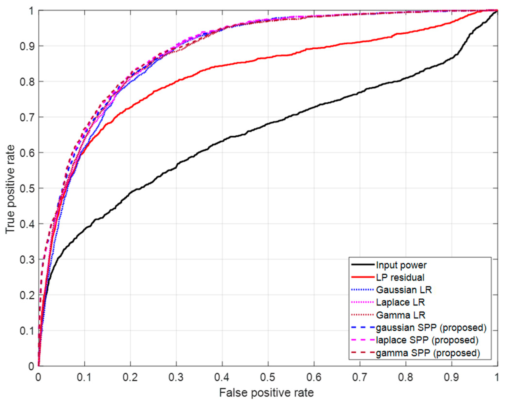
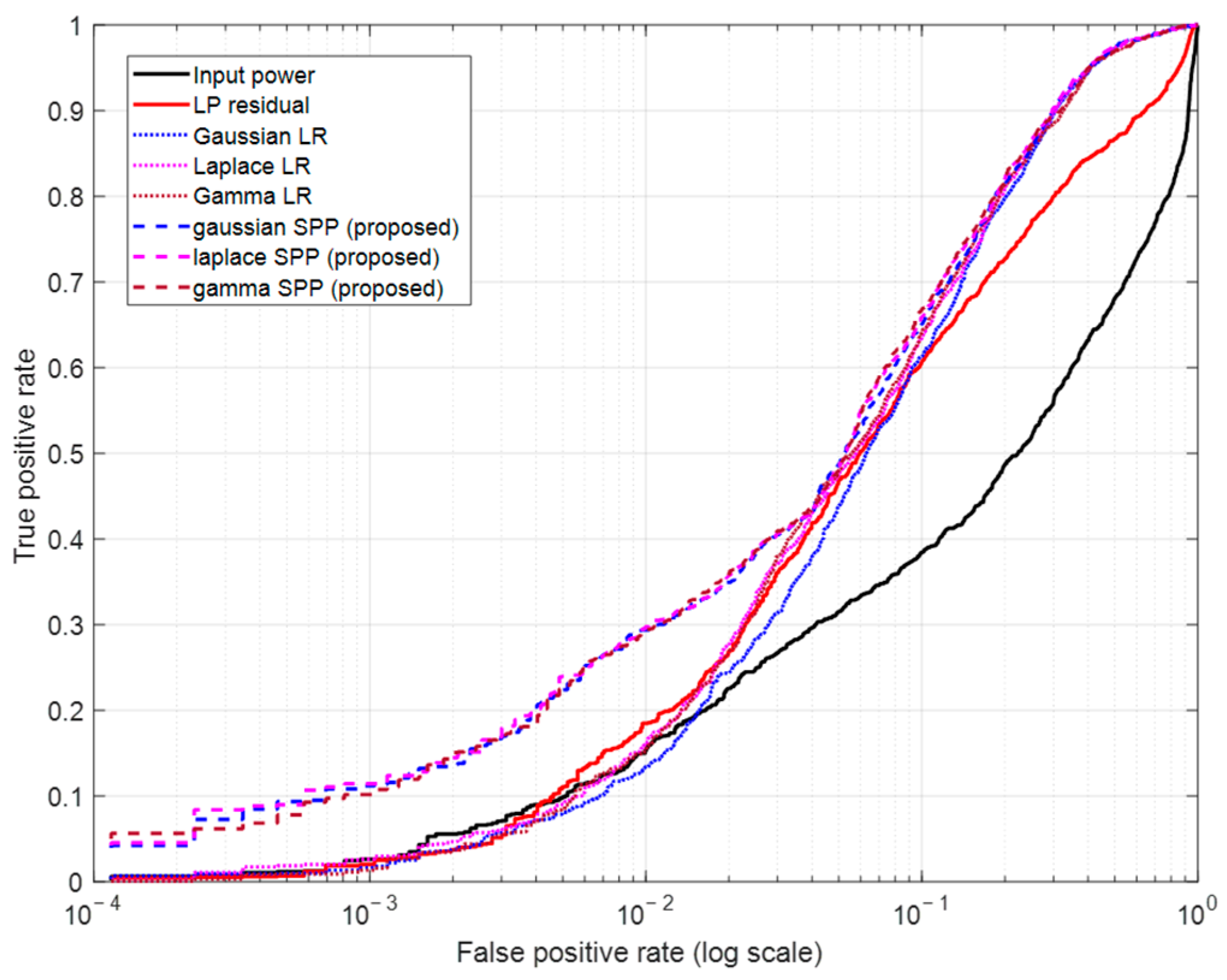
Furthermore, to confirm the results of Figure 5 numerically, ROC curves and AUCs [16] are presented in Figure 6 and Figure 7, as well as Table 1. In Figure 6, the ROC curves of the proposed SPPs are close to the left upper side, which is the best feature for discrimination. However, the difference between LRs and SPPs is slight. Thus, in order to look into the difference, Figure 7 is presented. When converting the False Positive Rate (FPR) from the linear scale to the logarithmic scale, it is confirmed that the proposed methods are superior to the LRs, especially when the FPR is below 0.04. Numerically, this performance improvement of the SPPs over LRs is supported by AUC, as presented in Table 1. The average performance improvement of SPPs over LRs is 0.0089.

4.2.2. SSN Reduction

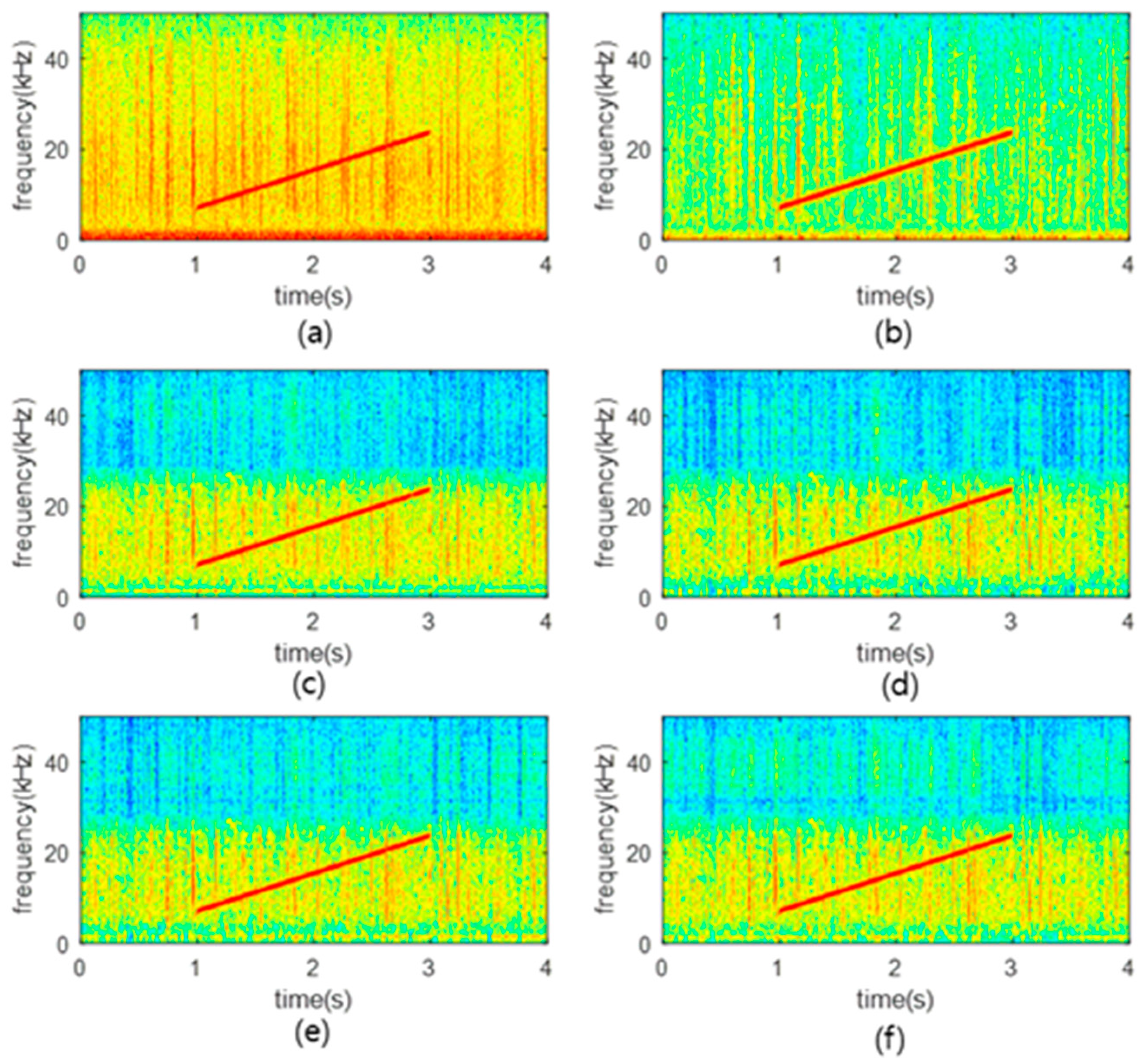
Subjectively, to verify the SSN reduction performance, spectrograms of noisy inputs, OM-LSA, NMF, and the proposed SPP-WNMFs are presented in Figure 8 and Figure 9. Overall, the noise reduction by all methods is successful compared to the noisy inputs. However, it is difficult to determine the superiority between OM-LSA and the other NMF-based methods because their spectrograms present very different patterns of noise reduction results. It can be confirmed that more noise has been removed because the colors of the SSN of the SPP-WNMF methods are lighter than that of the NMF.
Objectively, to evaluate the SSN reduction performance of the proposed and competing methods, overall/segmental SNRs, SDR, which indicates the ratio of defects such as artifacts and interference in the separated source from the original signal, and LSD, which represents the scale of signal distortion using the magnitude spectrum were measured and are summarized in Table 2, Table 3, Table 4, Table 5, Table 6, Table 7, Table 8 and Table 9.
Table 2 and Table 3 represent the overall SNR when the target signal and SSN are separated, and Table 4 and Table 5 represent the Segmental SNR. Based on the figures in the Tables, it can be seen that the proposed method shows higher SNR than the existing method. However, it is confirmed that the difference between proposed SPP-WNMFs is not significant because the difference in AUC was not significant as a result of detection. This tendency is similar to the SDRs presented in Table 6 and Table 7. From the SNR and SDR perspectives, the best results are obtained when Gaussian distribution-based SPP is applied as a weight when the target signal is CW. In addition, when the signal is LFM, the basis matrix size is (128:32), and the SNR is relatively low (−10, −5, 0 dB), the gamma distribution-based SPP-WNMF presented the best results, and when the SNR is relatively high (5, 10 dB), the Gaussian distribution-based SPP-WNMF presented the best results. Furthermore, when the basis matrix size is (128:64), Gaussian distribution-based SPP-WNMF presented the best results. Finally, from Table 8 and Table 9, we confirmed that LSD satisfies the lowest value of the three distributions when applying Gaussian distribution-based WNMF regardless of signal type.

5. Discussion

For SSN detection, we derived SPP by estimating a priori SAP and by incorporating it with the LRs in [15]. In light of our experience in acoustic signal processing, performance improvements by converting from LR to SPP were smaller than expected. To verify this, a similar test is performed in the speech area using NOIZEUS [29] data. As the results, we confirm that the performance of SPP is much higher than that of LR in speech interval detection. Applying a priori SAP likely increases detection discrimination as a feature for speech interval detection. However, LR itself has a high discrimination in SSN detection. Therefore, the role of a priori SAP is not that significant in improving the performance of SSN detection. Nevertheless, it is worth noting that SPP is an inherent weight that is bound between 0 and 1, is used for SSN reduction, and is a highly discriminative feature for SSN detection.
For SSN reduction, we proposed that WNMF employ SPP as weight information. As per the results, the proposed three SPP-WNMF methods (NMF(G), NMF(L), NMF(A)) presented superior performance to OM-LSA and NMF in all SNR conditions. However, when the signal is the LFM and the basis dimension is 32, the overall SNR performance of NMF is inferior to that of OM-LSA. This tendency appears in Table 3, whereas the proposed methods consistently perform well regardless of the signal type and the number of basis. Moreover, the performance improvements were high when the SOI was CW compared to LFM because CW is a narrowband signal and LFM is a wideband signal, making it easier to remove noise when the SOI is CW. In addition, using a sufficient number of basis allows for accurate reduction of SSN, but excessive basis allocation can increase the redundancy of the learned matrix and lead to the incorrect learning of noise characteristics; the experimental results showed that for the case of CW, the best performance was observed when the basis matrix sizes for SSN and the target signal were 128 and 32, respectively, whereas in case of the LFM, 128 for SSN and 64 for target signal were the best.
Comprehensively considering the experimental results, the proposed SPP-WNMFs consistently presented high SNR and SDR while satisfying low LSD compared to existing methods, which means successful noise reduction.

6. Conclusions

In this paper, we proposed a unified detection and reduction method for SSNs commonly encountered in underwater environments except in polar regions. This method detects the SSN interval probabilistically and uses the derived probability information for SSN reduction. In order to verify the effectiveness of the proposed method, experiments for SSN detection and reduction were performed using the SAVEX-15 dataset containing a large number of SSNs collected in a real ocean. As a result of the experiment, the proposed SPPs presented higher performance in SSN detection compared to the other competing methods. However, the performance improvements were not as high as expected, and it is considered that slight improvements from LRs to SPPs originated from the transient signal characteristics. In addition, it is confirmed that the SPP-WNMF method, which uses the SPP information for SSN reduction, outperforms the other existing methods. Nevertheless, the proposed SPP-based SSN detection and NMF-based SSN reduction are not optimal. Therefore, as future works, we will apply the latest machine learning and deep learning techniques to SSN detection and reduction for further performance improvement.

Author Contributions

Conceptualization, S.P. and J.H.; Data curation, S.P.; Funding acquisition, J.S.; Investigation, S.P.; Methodology, J.H.; Project administration, J.S. and J.H.; Software, S.P.; Writing—original draft, S.P.; Writing—review and editing, S.P. and J.H. All authors have read and agreed to the published version of the manuscript.

Funding

This work was supported by Korea Research Institute for defense Technology planning and advancement(KRIT) grant funded by the Korea government(DAPA(Defense Acquisition Program Administration)) (No. KRIT-CT-22-052, Physics-guided Intelligent Sonar Signal Detection Research Laboratory, 2024).

Institutional Review Board Statement

Not applicable.

Informed Consent Statement

Not applicable.

Data Availability Statement

Data are contained within the article.

Acknowledgments

We thank the Korea Research Institute of Ships and Ocean Engineering for providing the SAVEX 15 data.

Conflicts of Interest

The authors declare no conflicts of interest.

References

  1. Wicksten, M.K.; McClure, M.R. Snapping shrimps (Decapoda: Caridea: Alpheidae) from the Dampier Archipelago, western Australia. Rec. West. Aust. Mus. Suppl. 2007, 73, 61–83. [Google Scholar] [CrossRef]
  2. Everest, F.A.; Young, R.W.; Johnson, M.W. Acoustical characteristics of noise produced by snapping shrimp. J. Acoust. Soc. Am. 1948, 20, 137–142. [Google Scholar] [CrossRef]
  3. Kim, B.N.; Hahn, J.; Cho, B.K.; Kim, B.C. Snapping shrimp sound measured under laboratory conditions. Jpn. J. Appl. Phys. 2010, 49, 07HG04. [Google Scholar] [CrossRef]
  4. Versluis, M.; Schmitz, B.; Von der Heydt, A.; Lohse, D. How snapping shrimp snap: Through cavitating bubbles. Science 2000, 289, 2114–2117. [Google Scholar] [CrossRef]
  5. Beng, K.T.; Teck, T.E.; Chitre, M.; Potter, J.R. Estimating the spatial and temporal distribution of snapping shrimp using a portable, broadband 3-dimensional acoustic array. In Proceedings of the Oceans 2003, Celebrating the Past… Teaming toward the Future (IEEE Cat. No. 03CH37492), San Diego, CA, USA, 22–26 September 2003; Volume 5, pp. 2706–2713. [Google Scholar]
  6. Johnson, M.W.; Everest, F.A.; Young, R.W. The role of snapping shrimp (Crangon and Synalpheus) in the production of underwater noise in the sea. Biol. Bull. 1947, 93, 122–138. [Google Scholar] [CrossRef]
  7. Lee, D.H.; Choi, J.W.; Shin, S.; Song, H.C. Temporal Variability in Acoustic Behavior of Snapping Shrimp in the East China Sea and Its Correlation With Ocean Environments. Front. Mar. Sci. 2021, 8, 779283. [Google Scholar] [CrossRef]
  8. Zhou, Y.; Wang, R.; Yang, X.; Tong, F. Orthogonal Projection and Distributed Compressed Sensing Based Impulsive Noise Estimation for Underwater Acoustic OSDM Communication. IEEE Internet Things J. 2023, 10, 22279–22293. [Google Scholar] [CrossRef]
  9. Wang, S.; He, Z.; Niu, K.; Chen, P.; Rong, Y. New results on joint channel and impulsive noise estimation and tracking in underwater acoustic OFDM systems. IEEE Trans. Wirel. Commun. 2020, 19, 2601–2612. [Google Scholar] [CrossRef]
  10. Loye, D.P.; Proudfoot, D.A. Underwater Noise to Marine Life. J. Acoust. Soc. Am. 1946, 18, 446–449. [Google Scholar] [CrossRef]
  11. Kim, B.N.; Choi, B.K.; Kim, B.C.; Jung, S.K.; Park, Y.; Lee, Y.K. Seawater temperature and wind speeds dependences and diurnal variation of ambient noise at the snapping shrimp colony. In Proceedings of the IEEE 2012 Oceans, Yeosu, Republic of Korea, 21–24 May 2012; pp. 1–3. [Google Scholar]
  12. Park, J.D.; Doherty, J.F. A steganographic app-roach to sonar tracking. IEEE J. Ocean. Eng. 2018, 44, 1213–1227. [Google Scholar] [CrossRef]
  13. Park, J.; Hong, J. Snapping shrimp noise detection methods based on linear prediction analysis. IEEE Sens. J. 2023, 24, 1679–1686. [Google Scholar] [CrossRef]
  14. Song, H.C.; Kim, S.M.; Kim, B.N.; Nam, S. Shallow-water acoustic variability experiment 2015 (SAVEX15) in the northern East China Sea. J. Acoust. Soc. Am. 2016, 140, 3012. [Google Scholar] [CrossRef]
  15. Park, S.; Seok, J.; Hong, J. Snapping Shrimp Noise Detection Based on Statistical Model. J. Mar. Sci. Eng. 2023, 12, 42. [Google Scholar] [CrossRef]
  16. Hanley, J.A.; McNeil, B.J. The meaning and use of the area under a receiver operating characteristic (ROC) curve. Radiology 1982, 143, 29–36. [Google Scholar] [CrossRef] [PubMed]
  17. Virtanen, T. Monaural Sound Source Separation by Perceptually Weighted Non-Negative Matrix Factorization; Tampere University of Technology Tech. Rep.; Tampere University of Technology: Tampere, Finland, 2007. [Google Scholar]
  18. Lee, D.; Seung, H. Algorithms for non-negative matrix factorization. Adv. Neural Inf. Process. Syst. 2000, 13, 556–562. [Google Scholar]
  19. Lee, D.; Seung, H. Learning the parts of objects by nonnegative matrix factorization. Nature 1999, 401, 788–791. [Google Scholar] [CrossRef] [PubMed]
  20. Ozerov, A.; Févotte, C. Multichannel nonnegative matrix factorization in convolutive mixtures for audio source separation. IEEE Trans. Audio Speech Lang. Process. 2010, 18, 550–563. [Google Scholar] [CrossRef]
  21. Cohen, I. Optimal speech enhancement under signal presence uncertainty using log-spectral amplitude estimator. IEEE Signal Process. Lett. 2002, 9, 113–116. [Google Scholar] [CrossRef]
  22. Hirszhorn, A.; Dov, D.; Talmon, R.; Cohen, I. Transient interference suppression in speech signals based on the OM-LSA algorithm. In Proceedings of the IWAENC 2012, International Workshop on Acoustic Signal Enhancement, Aachen, Germany, 4–6 September 2012; pp. 1–4. [Google Scholar]
  23. Roux, J.; Wisdom, S.; Erdogan, H.; Hershey, J. SDR–half-baked or well done? In Proceedings of the IEEE International Conference on Acoustics, Speech and Signal Processing (ICASSP), Brighton, UK, 12–17 May 2019; pp. 626–630. [Google Scholar]
  24. Gray, A.; Markel, J. Distance measures for speech processing. IEEE Trans. Acoust. Speech Signal Process. 1976, 24, 380–391. [Google Scholar] [CrossRef]
  25. Makhoul, J. Linear prediction: A tutorial review. Proc. IEEE. 1975, 63, 561–580. [Google Scholar] [CrossRef]
  26. Chang, J.H.; Kim, N.S.; Mitra, S.K. Voice activity detection based on multiple statistical models. IEEE Trans. Signal Process. 2006, 54, 1965–1976. [Google Scholar] [CrossRef]
  27. Hu, Y.; Zhang, X.; Zou, X.; Min, G.; Sun, M.; Zheng, Y. Speech Enhancement Combining NMF Weighted by Speech Presence Probability and Statistical Model. IEICE Trans. Fundam. Electron. Commun. Comput. Sci. 2015, E98-A(12), 2701–2704. [Google Scholar] [CrossRef]
  28. Cohen, I.; Berdugo, B. Noise estimation by minima controlled recursive averaging for robust speech enhancement. IEEE Signal Process. Lett. 2002, 9, 12–15. [Google Scholar] [CrossRef]
  29. Hu, Y.; Loizou, P. Subjective evaluation and comparison of speech enhancement algorithms. Speech Commun. 2007, 49, 588–601. [Google Scholar] [CrossRef] [PubMed]
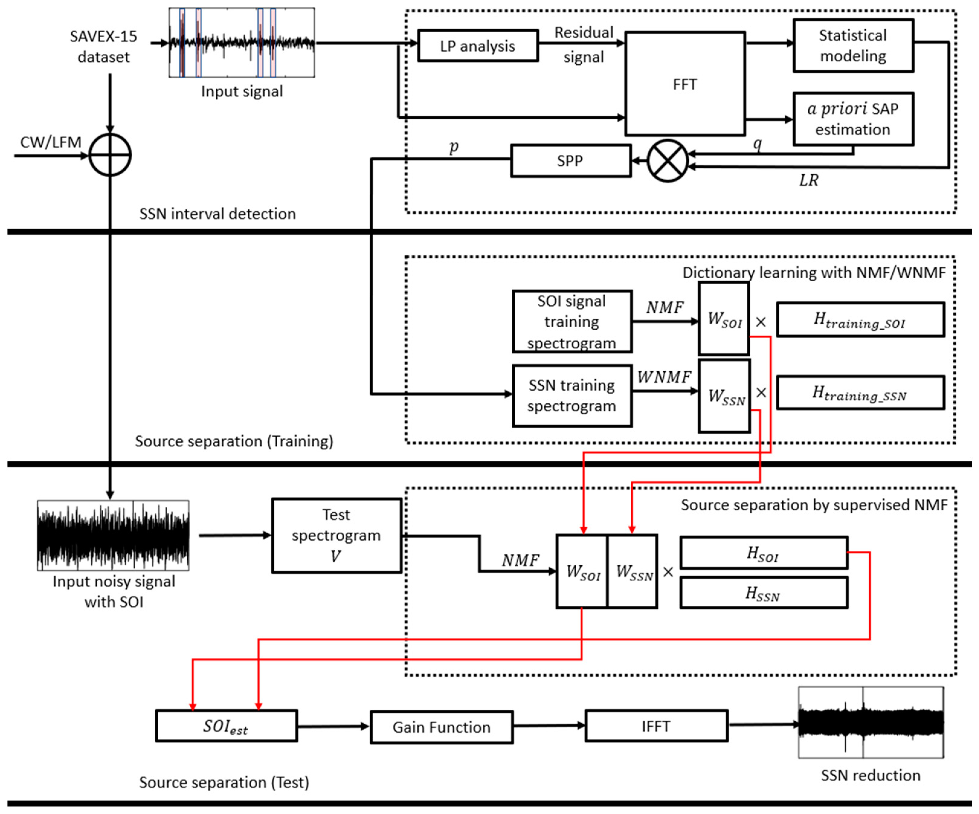
Figure 1. Entire block diagram of the proposed method.
Jmse 13 00096 g001
Figure 2. SAVEX-15 dataset collection environment.
Jmse 13 00096 g002
Figure 3. Hydrophone input samples (10 ms) in the SAVEX-15 dataset, marked in blue, all correspond to SSNs. (a) Time series of a hydrophone input, (b) spectrogram of (a).
Jmse 13 00096 g003
Figure 4. Spectrograms of synthesized noisy hydrophone inputs at SNR 0 dB: (a) CW, (b) LFM.
Jmse 13 00096 g004
Figure 5. Normalized feature contours (a) input signal, (b) input signal power, (c) LP residual, (d) statistical model-based LRs, (e) proposed SPPs (blue: Gaussian, purple: Laplace, brown: Gamma).
Jmse 13 00096 g005
Figure 6. ROC curves of input power, LP analysis [13], statistical model-based LRs [15], and proposed SPPs.
Jmse 13 00096 g006
Figure 7. Logarithmic scaled ROC curves of input power, LP analysis [13], statistical model-based LRs [15], and proposed SPPs.
Jmse 13 00096 g007
Figure 8. Results of SSN reduction when the target signal is CW (a): Noisy inputs (SNR 0 dB), (b): Transient OM-LSA based SSN reduction, (c): NMF based SSN reduction, (d): Gaussian WNMF based SSN reduction, (e): Laplace WNMF based SSN reduction, (f): Gamma WNMF based SSN reduction.
Jmse 13 00096 g008
Figure 9. Results of SSN reduction when the target signal is LFM (a): Noisy inputs (SNR 0 dB), (b): Transient OM-LSA based SSN reduction, (c): NMF based SSN reduction, (d): Gaussian WNMF based SSN reduction, (e): Laplace WNMF based SSN reduction, (f): Gamma WNMF based SSN reduction.
Jmse 13 00096 g009
Table 1. AUC results of LRs and SPPs.
AUCGaussianLaplaceGamma
LR0.88020.88570.8844
SPP0.89410.89350.8920
Table 2. Comparison of overall SNR(CW), G: Gaussian, L: Laplace, A: Gamma.
CWOM-LSABasis Matrix Size: (128:32)Basis Matrix Size: (128:64)
SNR NMFNMF(G)NMF(L)NMF(A)NMFNMF(G)NMF(L)NMF(A)
−100.125.947.387.367.735.495.905.886.49
−56.159.1811.1411.1711.488.9610.1510.1710.66
010.0312.8715.3315.4315.6812.7714.6214.6815.08
512.5617.0419.8119.9120.1316.9819.2619.3119.65
1013.7921.1824.1124.1724.3121.1523.7123.7323.97
Table 3. Comparison of overall SNR(LFM), G: Gaussian, L: Laplace, A: Gamma.
LFMOM-LSABasis Matrix Size: (128:32)Basis Matrix Size: (128:64)
SNR NMFNMF(G)NMF(L)NMF(A)NMFNMF(G)NMF(L)NMF(A)
−101.323.463.843.744.132.132.712.512.46
−56.015.827.227.057.396.727.427.247.20
09.737.8210.5810.3310.6111.1712.1511.9811.96
512.399.7314.0813.7513.9915.3816.9216.7516.76
1013.7111.6417.7817.4117.6319.1121.7121.5521.58
Table 4. Comparison of segmental SNR(CW), G: Gaussian, L: Laplace, A: Gamma.
CWNoisy InputOM-LSABasis Matrix Size: (128:32)Basis Matrix Size: (128:64)
SNR NMFNMF(G)NMF(L)NMF(A)NMFNMF(G)NMF(L)NMF(A)
−10−9.092.337.029.018.949.406.637.847.728.32
−5−4.559.1911.0513.5113.4513.9110.7912.5112.4112.99
00.4311.6915.5418.2818.2418.7015.3317.3617.2717.84
55.4313.2020.2923.1623.1223.5820.1022.2822.1822.74
1010.4213.9625.1228.0127.9628.4124.9427.1627.0627.61
Table 5. Comparison of segmental SNR(LFM), G: Gaussian, L: Laplace, A: Gamma.
LFMNoisy InputOM-LSABasis Matrix Size: (128:32)Basis Matrix Size: (128:64)
SNR NMFNMF(G)NMF(L)NMF(A)NMFNMF(G)NMF(L)NMF(A)
−10−9.094.604.555.425.225.525.066.315.975.85
−5−4.558.647.288.868.628.949.6310.9310.6210.54
00.4211.3010.1312.5512.2612.5814.2215.6115.3115.27
55.4213.0313.2316.5216.1916.5118.8520.3620.0720.05
1010.4213.8916.6220.7320.3620.6823.5125.1424.8624.87
Table 6. Comparison of SDR(CW), G: Gaussian, L: Laplace, A: Gamma.
CWNoisy InputOM-LSABasis Matrix Size: (128:32)Basis Matrix Size: (128:64)
SNR NMFNMF(G)NMF(L)NMF(A)NMFNMF(G)NMF(L)NMF(A)
−10−10.06−3.265.947.387.367.735.495.905.886.49
−5−5.035.959.1811.1411.1711.498.9610.1510.1610.66
0−0.029.9712.8715.3315.4315.6812.7714.6214.6815.08
54.9912.5317.0419.8119.9120.1316.9819.2619.3119.65
109.9913.7821.1824.1124.1724.3121.1523.7123.7323.97
Table 7. Comparison of SDR(LFM), G: Gaussian, L: Laplace, A: Gamma.
LFMNoisy InputOM-LSABasis Matrix Size: (128:32)Basis Matrix Size: (128:64)
SNR NMFNMF(G)NMF(L)NMF(A)NMFNMF(G)NMF(L)NMF(A)
−10−10.000.423.463.843.744.132.132.712.512.46
−5−5.005.895.827.227.057.396.727.427.247.20
00.009.697.8210.5810.3310.6111.1712.1511.9811.96
55.0012.369.7314.0813.7513.9915.3816.9216.7516.76
1010.0013.7011.6417.7817.4117.6319.1121.7121.5521.58
Table 8. Comparison of LSD(CW), G: Gaussian, L: Laplace, A: Gamma.
CWNoisy InputOM-LSABasis Matrix Size: (128:32)Basis Matrix Size: (128:64)
SNR NMFNMF(G)NMF(L)NMF(A)NMFNMF(G)NMF(L)NMF(A)
−1014.1112.9112.0411.8412.0111.9013.2813.1513.2513.24
−514.1112.4311.4211.2511.4111.3012.6712.5912.6912.67
013.8511.8810.7310.5910.7510.6511.9511.9212.0111.99
513.5611.4210.2310.1010.2510.1711.4011.3911.4811.47
1013.1410.969.779.649.789.7010.8710.8710.9610.94
Table 9. Comparison of LSD(LFM), G: Gaussian, L: Laplace, A: Gamma.
LFMNoisy InputOM-LSABasis Matrix Size: (128:32)Basis Matrix Size: (128:64)
SNR NMFNMF(G)NMF(L)NMF(A)NMFNMF(G)NMF(L)NMF(A)
−104.363.113.082.862.993.113.082.842.963.10
−54.382.812.712.512.632.722.802.562.682.80
04.252.442.282.112.212.282.432.202.312.42
53.932.041.871.741.811.872.051.851.932.03
103.501.681.511.411.471.511.691.521.591.66
Disclaimer/Publisher’s Note: The statements, opinions and data contained in all publications are solely those of the individual author(s) and contributor(s) and not of MDPI and/or the editor(s). MDPI and/or the editor(s) disclaim responsibility for any injury to people or property resulting from any ideas, methods, instructions or products referred to in the content.