Advanced Control for Shipboard Cranes with Asymmetric Output Constraints

Abstract

Considering the anti-swing control and output constraint problems of shipboard cranes, a nonlinear anti-swing controller based on asymmetric barrier Lyapunov functions (BLFs) is designed. First, model transformation mitigates the explicit effects of ship roll on the desired position and payload fluctuations. Then, a newly constructed BLF is introduced into the energy-based Lyapunov candidate function to generate nonlinear displacement and angle constraint terms to control the rope length and boom luffing angle. Among these, constraints with positive bounds are effectively handled by the proposed BLF. For the swing constraints of the unactuated payload, a carefully designed relevant constraint term is embedded in the controller by constructing an auxiliary signal, and strict theoretical analysis is provided by using a reductio ad absurdum argument. Additionally, the auxiliary signal effectively couples the boom and payload motions, thereby improving swing suppression performance. Finally, the asymptotic stability is proven using LaSalle’s invariance principle. The simulation comparison results indicate that the proposed method exhibits satisfactory performance in swing suppression control and output constraints. In all simulation cases, the payload swing angle complies with the 3° constraint and converges to the desired range within 6 s. This study provides an effective solution to the control challenges of shipboard crane systems operating in confined spaces, offering significant practical value and applicability.

1. Introduction

Shipboard cranes are essential in marine engineering, with broad applications in the construction and maintenance of offshore facilities [1], offshore resupply operations [2], and the loading and unloading of cargo on ships [3]. However, due to the complex dynamic characteristics of the system and harsh working conditions at sea, manual operation suffers from low efficiency and poor control precision. This fact has led to an urgent demand for the automated control of shipboard cranes, driving significant advancements in the field. Crane systems represent a class of underactuated systems where the number of control inputs is less than the number of outputs. They exhibit highly nonlinear and strongly coupled characteristics, posing considerable challenges to the design of automatic control methods [4,5]. Although substantial progress has been made in controlling land-based cranes [6,7,8,9,10,11,12,13,14], these methods cannot be directly or effectively applied to shipboard cranes. The added complexity of ship motion significantly increases the system’s dynamic complexity and internal coupling. Furthermore, the persistent disturbances caused by ocean waves and currents adversely affect the precise transportation of payloads and the suppression of swing.

In recent years, shipboard cranes have garnered significant attention in the control field, leading to many notable achievements [15]. The control methods explored in these studies can be broadly categorized into sliding mode control (SMC) [16,17,18], energy-based control [19,20,21], fuzzy logic [22,23], neural network control [24,25], and optimization-based control [26,27], among others. For instance, Kim et al. [18] proposed an adaptive SMC using the dynamics of shipboard cranes, demonstrating satisfactory disturbance rejection performance. Lu et al. [19] designed a nonlinear energy-based control method for shipboard cranes, incorporating the effects of both ship roll and heave motions. Unfortunately, existing studies rarely consider or effectively address the issue of output constraints, leaving a critical gap in developing advanced control strategies for shipboard boom cranes.

In practice, the limited workspace or stringent operational requirements often impose constraints on both actuated and unactuated output variables of crane systems, ensuring they remain within appropriate ranges [28]. For instance, the rope length must always remain positive and constrained within a specific range to prevent collisions during transportation. Furthermore, given the instability of the ship’s base and the relatively narrow workspace, it is crucial to ensure precise payload positioning while limiting payload swings to avoid accidents. Limiting payload swings can also effectively enhance system efficiency and reduce energy consumption. To address output constraints in underactuated systems, Li et al. [29] and Lu et al. [30] investigated the constraints on actuated variables. However, their studies neglected the more complex issue of constraints on unactuated states. Although Qian et al. [31] considered constraints on unactuated states, the designed controller theoretically only limited the payload swing angle within a conservative bounded range of (−π/2,π/2). Furthermore, Wang et al. [32] successfully constrained both the actuated and underactuated states within their respective predefined ranges, thereby ensuring limited overshoot and effective swing suppression performance. However, this method can only impose symmetric constraints on output states. In practice, some constraints are asymmetric, and some even share the same sign, such as positive rope length. Given the harsh working environment of shipboard cranes, these issues require urgent attention and are expected to be effectively addressed to ensure the reliability, efficiency, and safety of maritime transportation operations.

Based on the above discussion, this paper proposes a nonlinear anti-swing control method based on barrier Lyapunov functions (BLFs). First, to ensure the asymptotic stability of the closed-loop system, a controller based on the energy method is constructed. Then, to meet more precise practical output constraint requirements, the paper modifies and extends the symmetric BLF [28] to propose an asymmetric BLF to handle output constraints. For the constraint of the unactuated states, an auxiliary signal is cleverly constructed to embed the relevant constraint terms into the controller. Additionally, to enhance the anti-swing performance, this auxiliary signal fully couples the movement of the boom and the payload. The main advantages of this method are as follows:

• Due to unforeseen disturbances such as persistent waves, the ship’s motion can significantly amplify the crane’s cargo swing during operation. Therefore, this paper designs the controller and conducts theoretical analysis using the original complex nonlinear dynamic model to ensure more reliable performance.
• This method achieves asymmetric motion constraints for the boom and rope by appropriately modifying conventional symmetric barrier functions, ensuring the validity of the rope length under the same sign constraints. For the swing constraints of the unactuated payload, unlike traditional approaches, the proposed method introduces an auxiliary signal to embed the relevant constraint terms into the controller, supported by rigorous theoretical analysis through proof using a reductio ad absurdum argument. Consequently, in contrast to most existing crane-related studies [14,15,16,17,18,19,20,21,22,23,24], which assume the swing angle is confined within a conservative range of (−π/2, π/2), the proposed method removes this assumption. Instead, it flexibly constrains the swing angle within a reasonable range according to practical requirements, making it more adaptable and effective for cargo loading, unloading, and transportation tasks.
• Moreover, the proposed auxiliary signal ingeniously integrates information such as boom luffing velocity and payload swing angle-related information, demonstrating superior swing suppression capabilities compared to existing methods. Theoretical analysis and simulation results further verify that the proposed method can accurately position the payload and effectively limit its swing amplitude, which is of significant importance for the challenging operational environment of shipboard cranes.

The remainder of this paper is organized as follows: The “Section 2” explicitly presents the dynamic equations for the shipboard boom crane, its model transformation procedure, and the primary control objectives. Next, the “Section 3” explains the controller design approach and the asymptotic stability. Subsequently, the “Section 4” verifies the effectiveness of the suggested controller through numerical simulation and related analysis. Finally, the “Section 5” provides some concluding remarks.

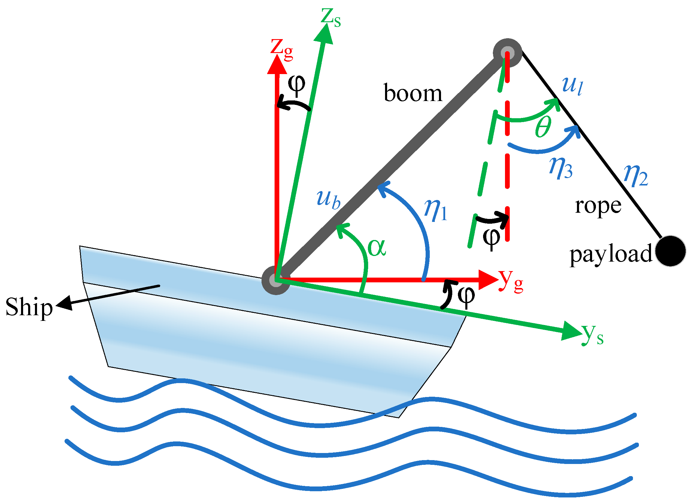
2. Problem Statement

2.1. Dynamics for Shipboard Boom Cranes

Figure 1 shows a schematic illustration of the shipboard boom crane system, featuring two coordination systems: the ground-fixed coordination system $y_g\text{-}O\text{-}{\mathrm{z}}_g$ and the ship-fixed coordination system $y_s\text{-}O\text{-}{\mathrm{z}}_s$. The system’s variables and parameters are listed in

Table 1. Parameters and variables.

Symbols	Parameters/Variables	Units
$\alpha$	Boom luffing angle	$\mathrm{rad}$
$\theta$	Payload swing angle	$\mathrm{rad}$
$\phi$	Ship rolling angle	$\mathrm{rad}$
$l$	Time-varying rope length	$\mathrm{m}$
$u_b$	Control input acting on the boom	$\mathrm{N}\cdot \mathrm{m}$
$u_l$	Control input acting on the rope	$\mathrm{N}$
$m_c$	Payload mass	$\mathrm{kg}$
$m_d$	The product of the boom mass and the distance between the boom barycenter and the point O	$\mathrm{kg}\cdot \mathrm{m}$
$b$	Boom length	$\mathrm{m}$
$J$	Boom rotational inertia	$\mathrm{kg}\cdot {\mathrm{m}}^2$
$g$	Gravity constant	${\mathrm{m}/\mathrm{s}}^2$

. The corresponding dynamic equation is given as follows [30]:

$$\mathit{M}(\mathit{q})\ddot{\mathit{q}}+\mathit{C}(\mathit{q},\dot{\mathit{q}})\dot{\mathit{q}}+\mathit{G}(\mathit{q})=\mathit{u}+{\mathit{\tau }}_d$$

(1)

where $\mathit{q}={[\begin{array}{ccc}\alpha & l& \theta \end{array}]}^{\top }\in {ℝ}^3$ is the state vector, $\mathit{M}(\mathit{q})\in {ℝ}^{3\times 3}$ and $\mathit{V}(\mathit{q},\dot{\mathit{q}})\in {ℝ}^{3\times 3}$ denote the inertia and centripetal-Coriolis matrices, respectively, $\mathit{G}(\mathit{q})\in {ℝ}^3$ represents the gravity vector, and $\mathit{u}={[\begin{array}{ccc}{u}_b& u_l& 0\end{array}]}^{\top }\in {ℝ}^3$ and ${\mathit{\tau }}_d\in {ℝ}^3$ represent the control input vector and perturbation vector, respectively. All elements contained in aforesaid matrices and vectors are given as

$$\mathit{M}=\left[\begin{array}{ccc}J+m_c{b}^2& -m_{c}b{C}_{\theta -\alpha }& m_{c}bl{S}_{\theta -\alpha }\\ -m_{c}b{C}_{\theta -\alpha }& m_c& 0\\ m_{c}bl{S}_{\theta -\alpha }& 0& m_c{l}^2\end{array}\right],$$

(2)

$$\mathit{C}=\left[\begin{array}{ccc}0& m_{c}b{S}_{\theta -\alpha }\dot{\theta }& c_{13}\\ -m_{c}b{S}_{\theta -\alpha }\dot{\alpha }& 0& -m_{c}l\dot{\theta }\\ -m_{c}bl{C}_{\theta -\alpha }\dot{\alpha }& m_{c}l\dot{\theta }& m_{c}l\dot{l}\end{array}\right],$$

(3)

$$\mathit{G}={[(m_{c}b+m_d)g{C}_{\alpha -\phi },-m_{c}g{C}_{\theta -\phi },m_{c}gl{S}_{\theta -\phi }]}^{\top },$$

(4)

$$\mathit{\tau }={\left[\begin{array}{c}(J+m_c{b}^2+m_{c}bl{S}_{\theta -\alpha })\ddot{\phi }+2m_{c}b\dot{l}{S}_{\theta -\alpha }\dot{\phi }-m_{c}bl{C}_{\theta -\alpha }({\dot{\phi }}^2-2\dot{\theta }\dot{\phi })\\ m_{c}l({\dot{\phi }}^2-2\dot{\theta }\dot{\phi })+m_{c}b{S}_{\theta -\alpha }({\dot{\phi }}^2-2\dot{\alpha }\dot{\phi })-m_{c}b{C}_{\theta -\alpha }\ddot{\phi }\\ m_{c}l(b{S}_{\theta -\alpha }+l)\ddot{\phi }+m_{c}bl{C}_{\theta -\alpha }({\dot{\phi }}^2-2\dot{\alpha }\dot{\phi })+2m_{c}l\dot{l}\dot{\phi }-{\tau }_r(\dot{\theta }-\dot{\phi })\end{array}\right]}^{\top },$$

(5)

where $c_{13}=mb(S_{\theta -\phi }\dot{l}+l{C}_{\theta -\phi }\dot{\theta })$, ${\tau }_r\in {ℝ}^{+}$ represents the damping coefficient. In addition, the symbols $S_{x-y}$ and $C_{x-y}$ ($x,y=\alpha ,\beta ,\phi$) represent functions $\sin (x-y)$ and $\cos (x-y)$, respectively.

As illustrated in Figure 1, the desired position of the payload in the coordination system $y_g\text{-}O\text{-}{\mathrm{z}}_g$ can be calculated as follows:

$$\begin{array}{l}{y}_d=b\cos ({\alpha }_d-\phi )+l_d\sin ({\theta }_d-\phi ),\\ z_d=b\sin ({\alpha }_d-\phi )-l_d\cos ({\theta }_d-\phi ),\end{array}$$

(6)

where ${\alpha }_d$, ${\theta }_d$, and $l_d$ represent the desired boom luffing angle, rope length, and payload swing angle, respectively. To eliminate the payload swing, we need ${\theta }_d=\phi (t)$. Therefore, we can derive the following:

$$\begin{array}{l}{\alpha }_d=\phi +arc\cos ({\displaystyle \frac{y_d}{b}}),\\ l_d=\sqrt{b^2-y_d^2}-z_d,{\theta }_d=\phi .\end{array}$$

(7)

It can be observed that ${\alpha }_d$, ${\theta }_d$, and $l_d$ are time-varying, which poses significant challenges in controller design. In order to simplify the subsequent analysis and calculations, new output states are defined as follows:

$$\mathit{\eta }={[\begin{array}{ccc}{\eta }_1& {\eta }_2& {\eta }_3\end{array}]}^{\top }={[\begin{array}{ccc}\alpha -\phi & l& \theta -\phi \end{array}]}^{\top }.$$

(8)

Together with Equations (7) and (8), the new states’ desired values can be expressed as follows:

$${\eta }_{1d}=\arccos ({\displaystyle \frac{y_d}{b}}),{\eta }_{2d}=\sqrt{b^2-y_d^2}-z_d,{\eta }_{3d}=0.$$

(9)

As shown in (9), the newly defined states eliminate the ship’s roll angle from (6), simplifying the subsequent analysis and calculations. Correspondingly, Equations (1)–(5) can be transformed into the following:

$$\mathit{M}(\mathit{\eta })\ddot{\mathit{\eta }}+\mathit{C}(\mathit{\eta },\dot{\mathit{\eta }})\dot{\mathit{\eta }}+\mathit{G}(\mathit{\eta })=\mathit{u}+{\mathit{\tau }}_{dn}$$

(10)

$$\mathit{M}=\left[\begin{array}{ccc}J+m_c{b}^2& -m_{c}b{C}_{1-3}& -m_{c}b{\eta }_2{S}_{1-3}\\ -m_{c}b{C}_{1-3}& m_c& 0\\ -m_{c}b{\eta }_2{S}_{1-3}& 0& m_c{l}^2\end{array}\right],$$

(11)

$$\mathit{C}=\left[\begin{array}{ccc}0& -m_{c}b{S}_{1-3}{\dot{\eta }}_3& c_{n13}\\ m_{c}b{S}_{1-3}{\dot{\eta }}_1& 0& -m_c{\eta }_2{\dot{\eta }}_3\\ -m_{c}b{\eta }_2{C}_{1-3}{\dot{\eta }}_1& m_c{\eta }_2{\dot{\eta }}_3& m_c{\eta }_2{\dot{\eta }}_2\end{array}\right],$$

(12)

$$\mathit{G}={[(m_{c}b+m_d)g{C}_1,-m_{c}g{C}_3,m_{c}gl{S}_3]}^{\top },$$

(13)

$${\mathit{\tau }}_{dn}={\left[\begin{array}{ccc}0& 0& -{\tau }_r{\dot{\eta }}_3\end{array}\right]}^{\top },$$

(14)

where $c_{n13}=mb(-S_{1-3}{\dot{\eta }}_2+{\eta }_2{C}_{1-3}{\dot{\eta }}_3)$, and the symbols $S_{i-j}$, $C_{i-j}$, $S_i$, and $C_i$ ($i,j=1,2,3$) represent functions $\sin ({\eta }_i-{\eta }_j)$, $\cos ({\eta }_i-{\eta }_j)$, $\sin ({\eta }_i)$, and $\cos ({\eta }_i)$, respectively.

It can be verified that $\mathit{M}(\mathit{\eta })$ in Equation (11) has the following property [27]:

$$\begin{array}{cc}{\mathit{x}}^{\top }\left[{\displaystyle \frac{1}{2}}\dot{\mathit{M}}(\mathit{\eta })-\mathit{C}(\mathit{\eta },\dot{\mathit{\eta }})\right]\mathit{x}=0,& \forall \mathit{x}\in {ℝ}^3\end{array}.$$

(15)

In practice, the initial values of the new state variables are within the preset ranges, i.e.,

$$\begin{array}{l}-{\displaystyle \frac{\pi }{2}}<m_1<{\eta }_1(0)<M_1<{\displaystyle \frac{\pi }{2}},\\ 0<m_2<{\eta }_2(0)<M_2,\\ -{\displaystyle \frac{\pi }{2}}<m_3<{\eta }_3(0)<M_3<{\displaystyle \frac{\pi }{2}},\end{array}$$

(16)

where $M_i,m_i,i=1,2,3$ represent the states’ allowable minimum and maximum values, respectively. For instance, $m_2$ and $M_2$ denote the permissible shortest and longest cable lengths greater than zero to comply with practical operational requirements.

2.2. Control Objective

For the shipboard crane system (10), we aim to design an appropriate controller $\mathit{u}$ to achieve the following objectives:

In the fixed ground coordinate system, transport the payload from its initial position to its desired position while eliminating residual payload swing, that is, make the new output state vector $\mathit{\eta }$ converge to its desired value ${\mathit{\eta }}_d$, which is expressed as follows:

$$\underset{t\to \infty }{\lim }{\eta }_1={\eta }_{1d},\underset{t\to \infty }{\lim }{\eta }_2={\eta }_{2d},\underset{t\to \infty }{\lim }{\eta }_3={\eta }_{3d}.$$

(17)

Considering the operational safety, limited workspace, and other specific requirements, the system’s new output state vector $\mathit{\eta }$ is constrained within the preset range throughout the operation, which can be described as follows:

$$\left\{\begin{array}{cc}\begin{array}{l}-{\displaystyle \frac{\pi }{2}}<m_1<{\eta }_1(t)<M_1<{\displaystyle \frac{\pi }{2}},\\ 0<m_2<{\eta }_2(t)<M_2,\\ -{\displaystyle \frac{\pi }{2}}<m_3<{\eta }_3(t)<M_3<{\displaystyle \frac{\pi }{2}},\end{array}& \forall \mathrm{t}\ge 0.\end{array}\right.$$

(18)

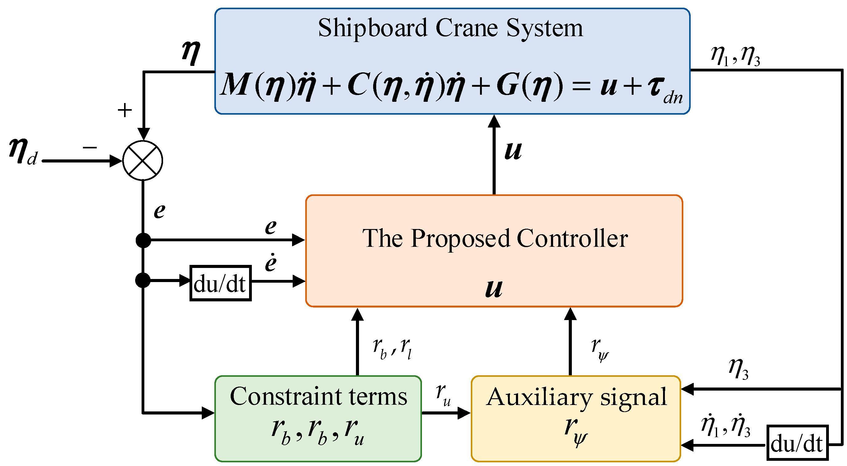
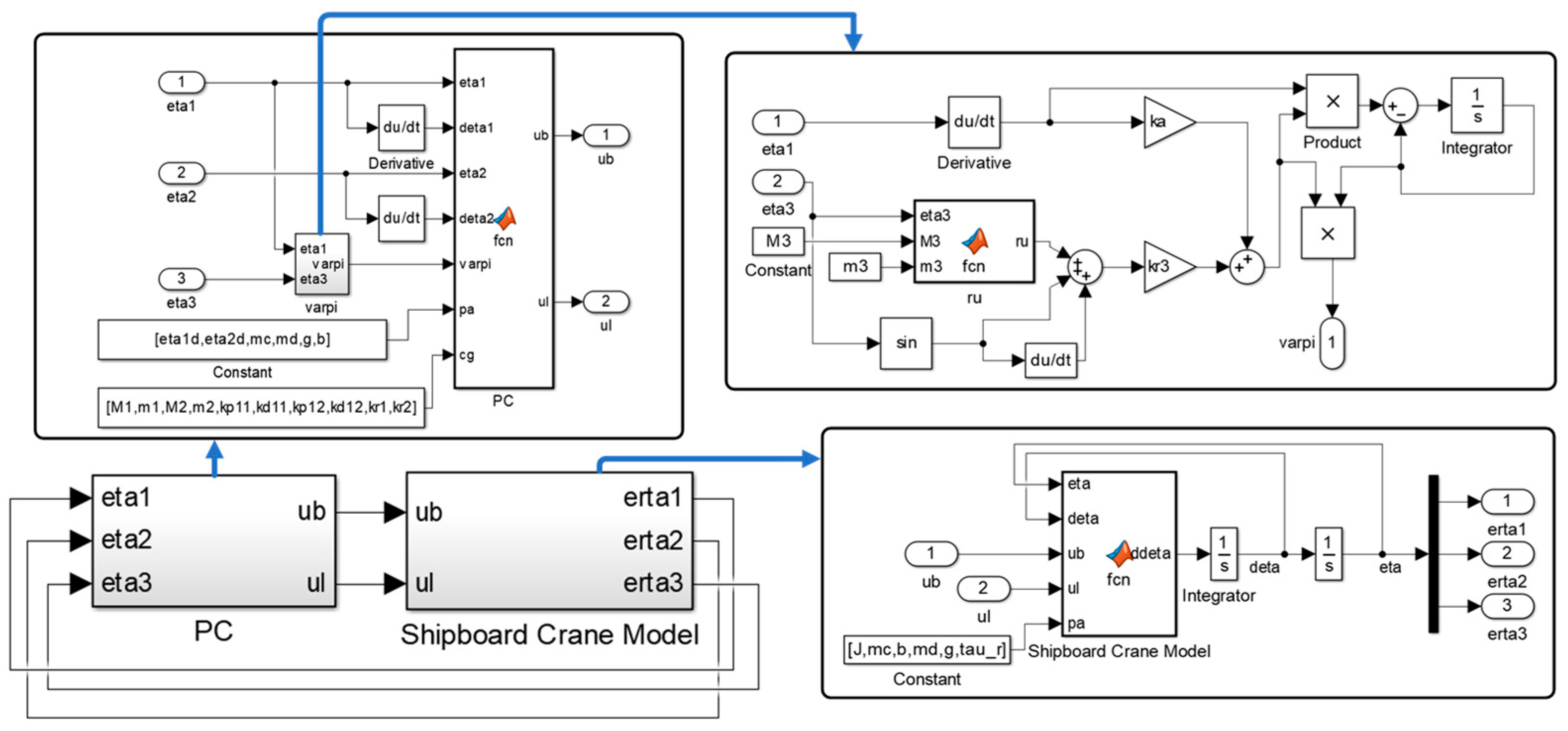
3. Controller Design and Stability Analysis

In this section, we propose a novel and efficient controller to achieve the objectives above, and we rigorously validate its effectiveness through theoretical analysis.

3.1. Controller Design

First, using Equations (9) and (17), we introduce the following error signals:

$$e_1={\eta }_1-{\eta }_{1d},e_2={\eta }_2-{\eta }_{2d},e_3={\eta }_3-{\eta }_{3d}={\eta }_3,$$

(19)

and correspondingly,

$${\dot{e}}_1={\dot{\eta }}_1,{\dot{e}}_2={\dot{\eta }}_2,{\dot{e}}_3={\dot{\eta }}_3.$$

(20)

Second, we construct the storage energy of the shipboard crane system as

$$E={\displaystyle \frac{1}{2}}{\dot{\mathit{q}}}^{\top }\mathit{{\rm M}}(\mathit{\eta })\dot{\mathit{q}}+m_{c}gl[1-\cos (\theta )],$$

(21)

and based on this, we replace $\mathit{q}$, $l$, and $\theta$ in Equation (21) with $\mathit{\eta }$, ${\eta }_2$, and ${\eta }_3$, respectively, to obtain the following storage function:

$$E_0={\displaystyle \frac{1}{2}}{\dot{\mathit{\eta }}}^{\top }{\rm M}(\mathit{\eta })\dot{\mathit{\eta }}+m_{c}g{\eta }_2[1-\cos ({\eta }_3)].$$

(22)

Then, differentiating $E_0$ in Equation (22) produces

$$\begin{array}{ll}{\dot{E}}_0& ={\dot{\mathit{\eta }}}^{\top }[\mathit{{\rm M}}(\mathit{\eta })\ddot{\mathit{\eta }}+\mathit{C}(\mathit{\eta },\dot{\mathit{\eta }})\dot{\mathit{\eta }}]\\ & +{\dot{\mathit{\eta }}}^{\top }[{\displaystyle \frac{1}{2}}\dot{\mathit{{\rm M}}}(\mathit{\eta })-\mathit{C}(\mathit{\eta },\dot{\mathit{\eta }})]\dot{\mathit{\eta }}\\ & +m_{c}g{\dot{\eta }}_2[1-\cos ({\eta }_3)]+m_{c}g{\eta }_2\sin ({\eta }_3){\dot{\eta }}_3,\end{array}$$

(23)

and based on the property (15) and the system model (10), we obtain

$$\begin{array}{ll}{\dot{E}}_0& ={\dot{\mathit{\eta }}}^{\top }[\mathit{u}+{\mathit{\tau }}_{dn}-\mathit{G}(\mathit{\eta })]\\ & +m_{c}g{\dot{\eta }}_2[1-\cos ({\eta }_3)]+m_{c}g{\eta }_2\sin ({\eta }_3){\dot{\eta }}_3.\end{array}$$

(24)

Substituting (13) and (14) into (24) yields

$$\begin{array}{c}{\dot{E}}_0=[u_b-(m_{c}b+m_d)g{C}_1]{\dot{\eta }}_1+\\ (u_l+m_{c}g){\dot{\eta }}_1-{\tau }_r{\dot{\eta }}_3^2.\end{array}$$

(25)

To effectively constrain the output states, we establish the following auxiliary signals:

$$\begin{array}{ll}{r}_b(e_1)& =e_1\log [({\eta }_1-m_1)/(M_1-{\eta }_1)]\{(M_1-m_1)e_1/[({\eta }_1-m_1)(M_1-{\eta }_1)]\\ & +\log [({\eta }_1-m_1)/(M_1-{\eta }_1)]\},\end{array}$$

(26)

$$\begin{array}{ll}{r}_l(e_2)& =e_2\log [({\eta }_2-m_2)/(M_2-{\eta }_2)]\{(M_2-m_2)e_2/[({\eta }_2-m_2)(M_2-{\eta }_2)]\\ & +\log [({\eta }_2-m_2)/(M_2-{\eta }_2)]\},\end{array}$$

(27)

$$r_u({\eta }_3)=\log [({\eta }_3-m_3)/(M_3-{\eta }_3)],$$

(28)

where $r_b$, $r_l$, and $r_u$ represent the constraint terms for the new states: the boom luffing angle ${\eta }_1$, the rope length ${\eta }_2$, and the underactuated payload swing angle ${\eta }_3$, respectively. Here, $\log$ stands for natural logarithm function.

In general, appropriately enhancing the dynamic coupling between the boom and payload facilitates damping injection, and one potential method to achieve this is to combine them into a composite signal [9]. Therefore, based on (28), we construct the following new composite signal:

$$r_{\psi }({\dot{\eta }}_1,{\eta }_3,{\dot{\eta }}_3)=k_{r3}[r_u+\sin ({\eta }_3)+\cos ({\eta }_3){\dot{\eta }}_3]+k_a{\dot{\eta }}_1$$

(29)

where $k_{r3}$ and $k_a$ are positive constants.

Therefore, in order to effectively constrain the system motion and utilize the designed coupling characteristics (29) to improve the system transient performance, we designed the following controller, and the corresponding control scheme diagram is shown in Figure 2.

$$\begin{array}{ll}{u}_b& =-k_{p1}{e}_1-k_{d1}{\dot{\eta }}_1+(m_{c}b+m_d)g{C}_1\\ & -k_{r1}{r}_b-r_{\psi }\varpi ,\\ u_l& =-k_{p2}{e}_2-k_{d2}{\dot{\eta }}_2-m_{c}g-k_{r2}{r}_l,\end{array}$$

(30)

with

$$\dot{\varpi }=-\varpi +r_{\psi }{\dot{\eta }}_1,$$

(31)

where $k_{p1},k_{d1},k_{p2},k_{d2},k_{r1},k_{r2}\in {ℝ}^{+}$ are positive control gains to be adjusted.

Note that the controller proposed in (30) does not exhibit any singularities, as will be demonstrated in the subsequent Stability Analysis.

Remark 1.

This paper proposes a novel barrier function to address the issue of asymmetric output constraints in nonlinear systems, such as the constraint on the boom luffing angle in (26), the constraint on cable length in (27), and the constraint on the underactuated payload’s swing angle in (29). Notably, unlike conventional approaches to handling underactuated state constraints [28,32], this study embeds the relevant constraint term (29) into the controller by constructing an auxiliary signal (31), which significantly simplifies the complexity of controller design and provides valuable insights for designing controllers and applying them in practice in future work. Moreover, the constructed auxiliary signal intentionally strengthens the dynamic coupling between the boom and payload, further enhancing the damping effect on the payload swing.

Remark 2.

Based on the tuning guidelines of PID controllers, the control gains k_p1, k_d1, k_p2, and k_d2 can be appropriately selected. Additionally, k_r1, k_r2, k_r3, and k_a, associated with the auxiliary constraint terms, can be selected as small positive values through a straightforward trial-and-error approach.

3.2. Stability Analysis

Theorem 1.

Under the continuous ship movement induced by ocean wave effects, the proposed controller (30) ensures that the system satisfies the constraints in (18) and achieves the control objective described in (17).

Proof of Theorem 1.

Based on (22), we choose

$$\begin{array}{cc}V& =E_0+{\displaystyle \frac{1}{2}}{k}_{p1}{e}_1^2++{\displaystyle \frac{1}{2}}{\varpi }^2+{\displaystyle \frac{1}{2}}{k}_{p2}{e}_2^2+{\displaystyle \frac{1}{2}}{k}_{r1}{\{\log [({\eta }_1-m_1)/(M_1-{\eta }_1)]e_1\}}^2\\ & +{\displaystyle \frac{1}{2}}{k}_{r2}{\{\log [({\eta }_2-m_2)/(M_2-{\eta }_2)]e_2\}}^2.\end{array}$$

(32)

Then, take the time derivative of (32) and consider (25) to obtain

$$\dot{V}=[u_b+k_{p1}{e}_1-(m_{c}b+m_d)g{C}_1+k_{r1}{r}_b]{\dot{\eta }}_1+[u_l+m_{c}g+k_{p2}{e}_2+k_{r2}{r}_l]{\dot{\eta }}_2-{\tau }_r{\dot{\eta }}_3^2+\varpi \dot{\varpi }.$$

(33)

By substituting the results of (30) and (31) into (33), one can yield that

$$\dot{V}=-k_{d1}{\dot{\eta }}_1^2-{\varpi }^2-k_{d2}{\dot{\eta }}_2^2-{\tau }_r{\dot{\eta }}_3^2.$$

(34)

Obviously,

$$\dot{V}\le 0.$$

(35)

Hence, we can confirm

$$V(t)\le V(0)\ll +\infty .$$

(36)

Furthermore, we can prove the following two items through (36):

• Assume that ${\eta }_1$ or ${\eta }_2$ reach its preset upper or lower limit at time $T$. In this case, the logarithmic terms corresponding to these states in $V$ would approach infinity, leading to $V(T)$ being infinite. This conclusion contradicts the result (36). Using a reductio ad absurdum argument, the states ${\eta }_1$ and ${\eta }_2$ are always able to comply with their constraints, that is,

  $$-{\displaystyle \frac{\pi }{2}}<m_1<{\eta }_1<M_1<{\displaystyle \frac{\pi }{2}},0<m_2<{\eta }_2<M_2$$

  (37)
• Assuming that ${\eta }_3$ violates any constraint within a very small adjacent time $t\in [T_1,T_2]$, referring to (28) and (29), $r_{\psi }$ will be infinite. And for $t\in [T_1,T_2]$, the solution of the differential Equation (31) is

$$\varpi (T_2)=\varpi (T_1)e^{-(T_2-T_1)}+{\displaystyle {\int }_{T_1}^{T_2}{r}_{\psi }(\rho ){\dot{\eta }}_1(\rho )e^{-(T_2-\rho )}d\rho }\to \infty ,as{\eta }_3\to m_{3}or{\mathrm{M}}_3,$$

(38)

which contradicts the result (36). Once again, using a reductio ad absurdum argument, the state variable ${\eta }_3$ is always able to comply with its constraints, that is,

$$-{\displaystyle \frac{\pi }{2}}<m_3<{\eta }_3<M_3<{\displaystyle \frac{\pi }{2}}$$

(39)

Considering the results of (37) and (39), the new state vector $\mathit{\eta }$ always satisfies its preset constraints, i.e., the objective described in (18). These results also show that the proposed controller will not have singularities and

$$V\ge 0$$

(40)

From (36) to (40), we can easily observe that

$$\begin{array}{ll}V(t)\in L_{\infty }\to & {\dot{\eta }}_1,{\dot{\eta }}_2,{\dot{\eta }}_3,e_1,e_2,e_3,\log [({\eta }_1-m_1)/(M_1-{\eta }_1),\\ & \log [({\eta }_2-m_2)/(M_2-{\eta }_2),\varpi \in L_{\infty }.\end{array}$$

(41)

Then, according to the controller formulas expressed in (26)–(30), we can infer

$$u_b,u_l\to L_{\infty }$$

(42)

Substituting the results of (41) and (42) into formula (10), we obtain

$${\ddot{\eta }}_1,{\ddot{\eta }}_2,{\ddot{\eta }}_3\in L_{\infty }$$

(43)

Next, we discuss the stability of system (10) with the controller (30) by using the LaSalle invariance theorem [33]. Let $\mathsf{\Phi }$ be the largest invariant set in $\mathrm{\Xi }$, where

$$\mathrm{\Xi }=\{\mathit{\eta },\dot{\mathit{\eta }}|\dot{V}=0\}.$$

(44)

Then, from the results of (34) and (35), one can conclude that in $\mathsf{\Phi }$,

$${\dot{\eta }}_1,{\dot{\eta }}_2,{\dot{\eta }}_3,\varpi =0\to {\ddot{\eta }}_1,{\ddot{\eta }}_2,{\ddot{\eta }}_3=0.$$

(45)

Substituting (45) into (10) and using the results of (13), (14), and (30), we obtain

$$\begin{array}{c}-k_{p1}{e}_1-k_{r1}{r}_b(e_1)=0\to e_1=0,\\ -k_{p2}{e}_2-k_{r2}{r}_l(e_2)=m_{c}g(1-C_3),\\ m_{c}gl{S}_3=0.\end{array}$$

(46)

According to the result of (39) and the property of the sine function, we can infer that

$$S_3=0\to {\eta }_3=0,e_3=0.$$

(47)

Hence,

$$-k_{p2}{e}_2-k_{r2}{r}_l(e_2)=m_{c}g(1-C_3)=0\to e_2=0.$$

(48)

From Equations (45)–(48), it can be concluded that the largest invariant set $\mathrm{\Xi }$ consists solely of the equilibrium point. Hence, states $\mathit{\eta }$ and $\dot{\mathit{\eta }}$ converge asymptotically to their desired values. Finally, by combining the results of (37) and (39), Theorem 1 is proved. □

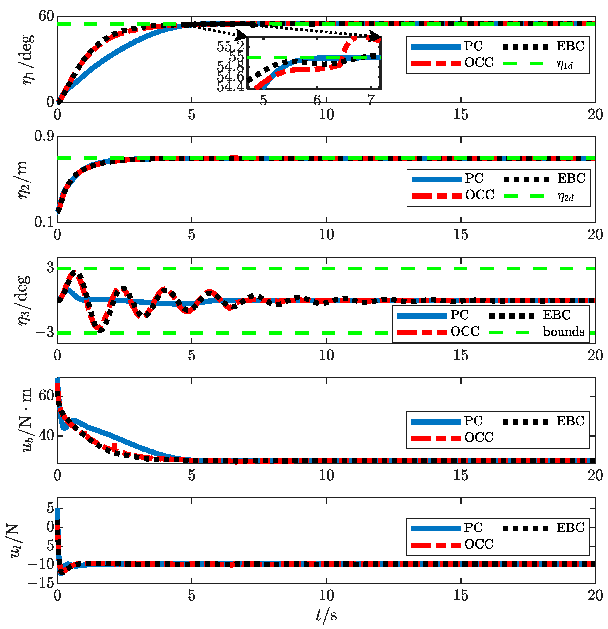
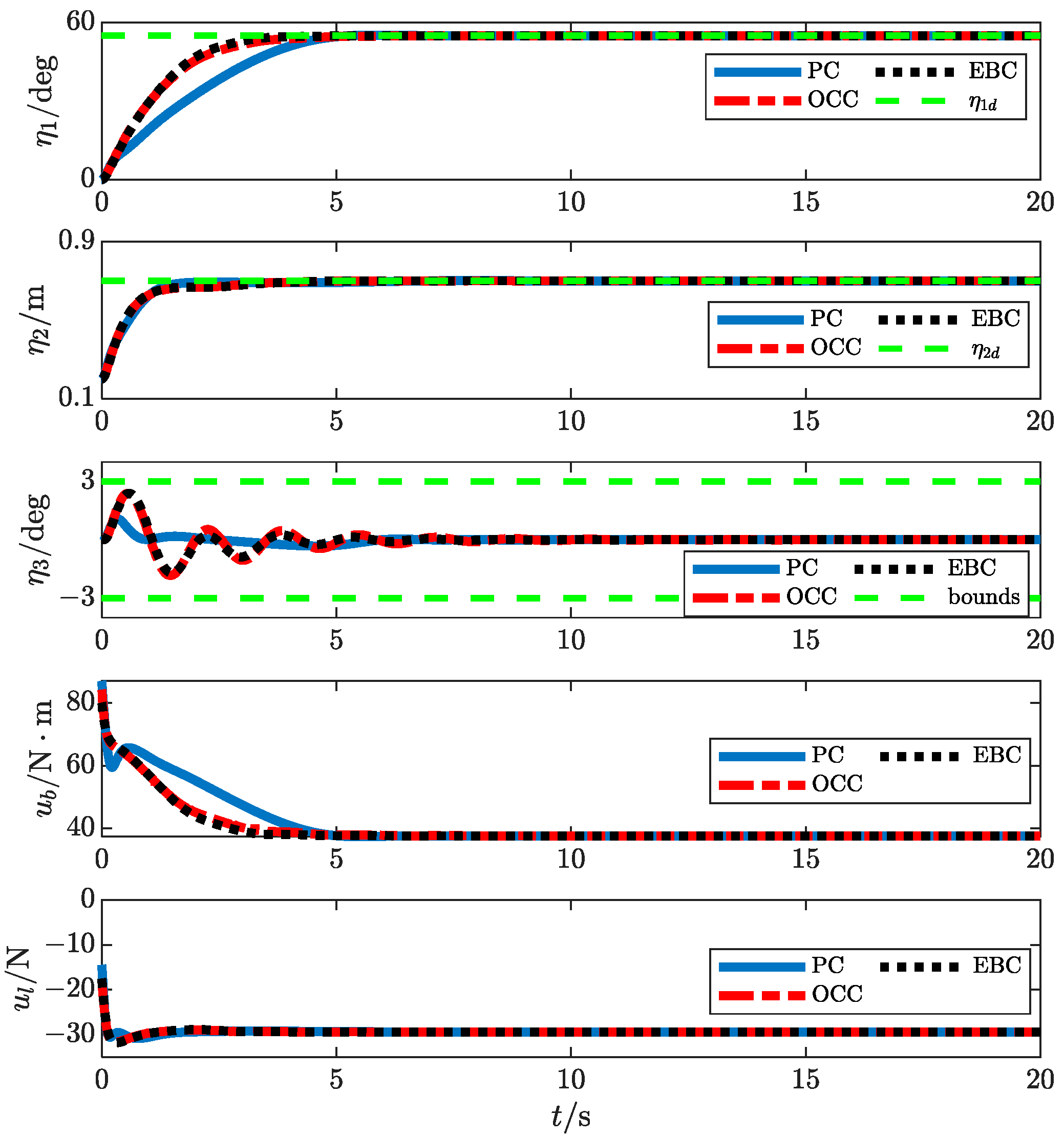
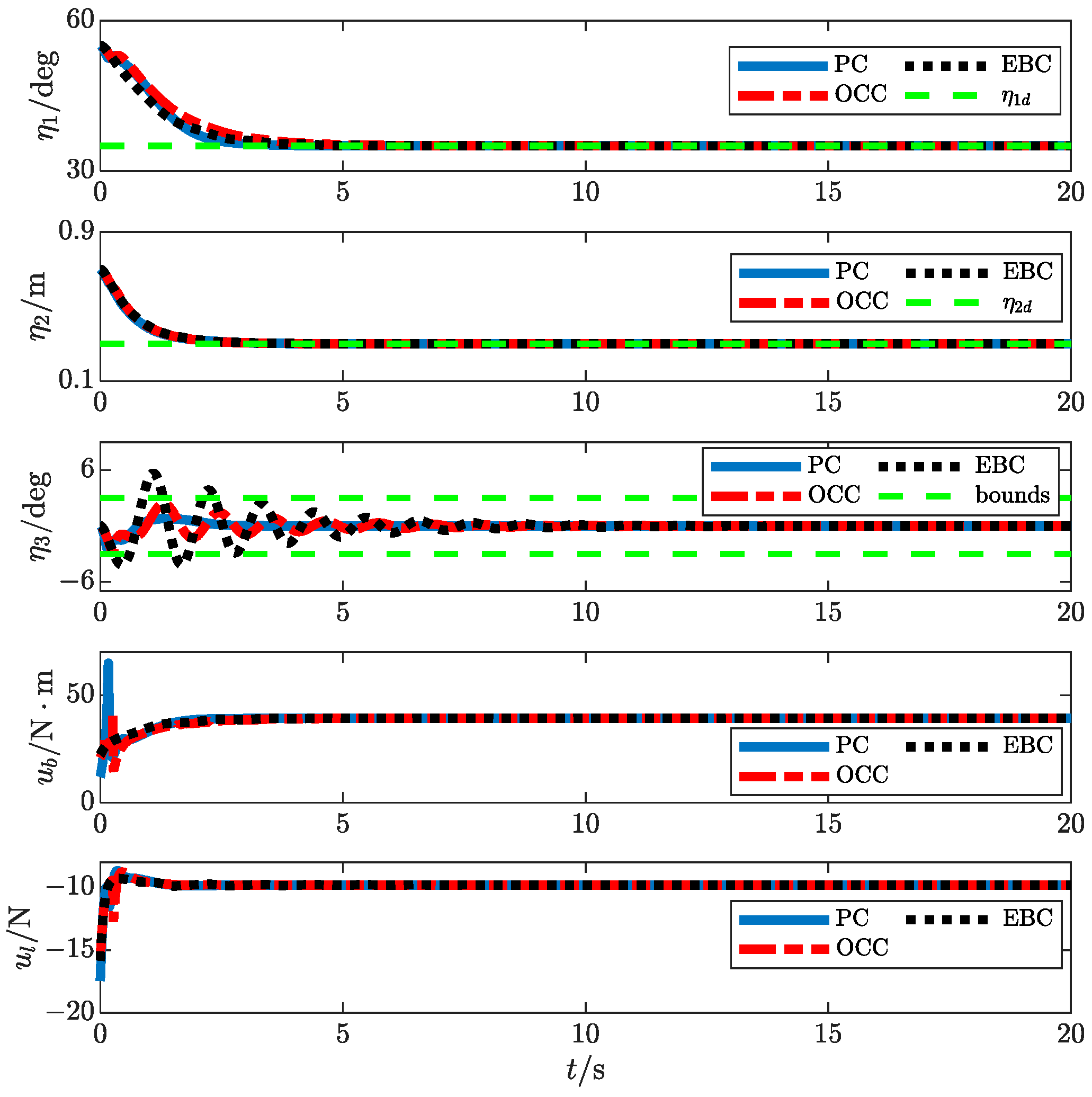
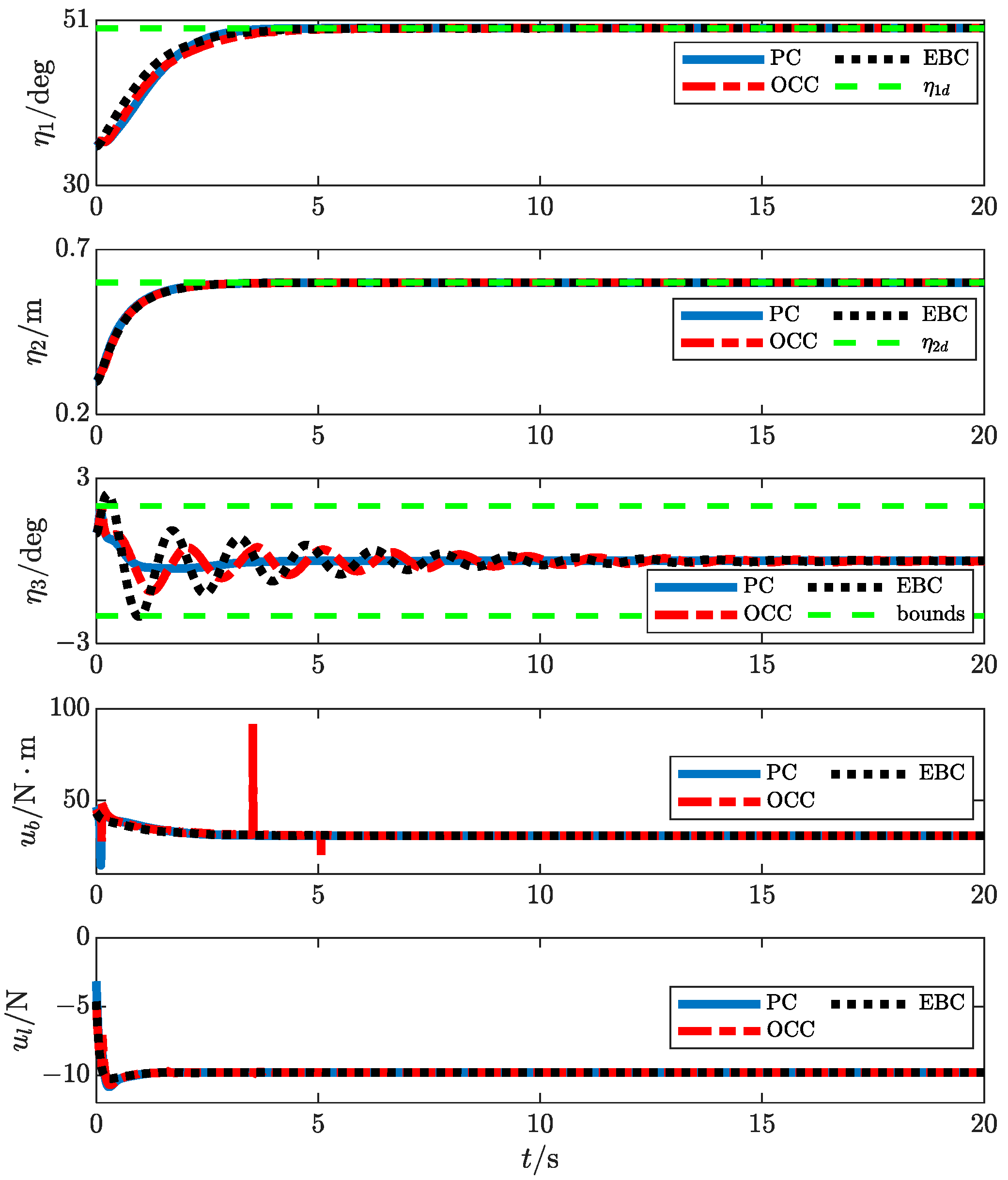
4. Simulation Results

To verify the effectiveness and evaluate the performance of the proposed controller in (30), we set up three simulations based on the MATLAB/Simulink R2014b platform (MathWorks, Natick, MA, USA). The solver was set to ODE3 (Bogacki-Shampine) with a fixed step size of 5 ms. The simulations were run on a computer equipped with an Intel(R) Core(TM) i7-12700H CPU (Intel Corporation, Santa Clara, CA, USA) operating at 2.30 GHz, 16 GB of RAM, an NVIDIA GeForce RTX 3060 Laptop GPU (NVIDIA Corporation, Santa Clara, CA, USA) with 6 GB of VRAM, and the Microsoft Windows 11 operating system (Microsoft Corporation, One Microsoft Way, Redmond, WA, USA).

Figure 3 illustrates the control scheme implemented in the MATLAB/Simulink simulation platform. The detailed implementation of the theoretical model (10)–(14) is located in the lower-right corner of the figure. The entire control scheme utilizes built-in Simulink library blocks, including the “Integrator”, “Derivative”, “Constant”, “In1”, “Out1”, “Demux”, “MATLAB Function”, “Gain”, “Product”, and “Sum”.

In the simulations, to thoroughly verify the effectiveness and performance of the proposed controller, we selected the existing advanced nonlinear anti-swing controllers [30,32] for shipboard boom cranes as benchmarks. Among them, the energy-based controller [30] is similar to PD control and has typical control performance, so the comparison results can intuitively reflect the control effect of the proposed controller; the controller with output constraints [32] has the ability to process symmetrical constraints of output states, which is in sharp contrast to the asymmetric output constraints processing ability of the proposed controller, thereby further verifying the advantage of the proposed controller in constraints processing and the transient performance improvement effect brought by this advantage. For the convenience of description, we denote the energy-based controller [30] as EBC, the controller with output constraints [32] as OCC, and the proposed controller as PC.

To facilitate the analysis of the simulation results, we first define the following performance indicators:

• $t_p$: The time required for the positioning error of the rope length to converge within the range of $(-0.004\mathrm{m},0.004\mathrm{m})$
• ${\eta }_{3\max }$: The payload swing amplitude’s peak value during the control process.
• $t_c$: The time required for the payload swing angle to converge within the range of $(-0.04°,0.04°)$

Group 1.

Performance Comparison. To intuitively reflect the performance of the proposed controller (28), we compare it with EBC and OCC without any disturbances. The simulation parameters are set as follows:

The main physical parameters of the shipboard crane system are as follows:

$$\begin{array}{l}{m}_c=1.0\mathrm{kg},\mathrm{b}=0.9\mathrm{m},m_d=4.0\mathrm{kg}\cdot \mathrm{m},\\ J=2.7\mathrm{kg}\cdot {\mathrm{m}}^2,g=9.8,{\tau }_r=0.05.\end{array}$$

The initial values and desired values of the new states are as follows:

$$\begin{array}{l}{\eta }_1(0)=0 \mathrm{deg},{\eta }_2(0)=0.1\mathrm{m},{\eta }_3(0)=0,\\ {\eta }_{1d}=55 \mathrm{deg},{\eta }_{2d}=0.7\mathrm{m},{\eta }_{3d}=0\mathrm{deg}.\end{array}$$

The state constraints are as follows:

$$\begin{array}{l}{\eta }_1\in (-55\mathrm{deg},60 \mathrm{deg}),{\eta }_2\in (0.1\mathrm{m},0.9\mathrm{m}),\\ {\eta }_3\in (-3\mathrm{deg},3 \mathrm{deg}).\end{array}$$

To ensure the results are comparable when tuning the controller gains, we first ensure the convergence of all states; then, we adjust the convergence times of ${\eta }_1$ and ${\eta }_2$ in all three controllers to be similar without intentionally introducing overshoot; finally, we focus on comparing the convergence performance of ${\eta }_3$ and the controllers’ output constraint capabilities. After careful tuning, the nominal control parameters of PC, EBC, and OCC are selected, as shown in

Table 2. Control gains for PC, EBC, and OCC.

Controllers	Control Gains
PC	$\begin{array}{l}{k}_{p1}=22,k_{d1}=21,k_{r1}=1,k_{r3}=6,k_a=16,k_{p2}=15,\\ k_{d2}=11,k_{r2}=1,M_1=60\mathrm{deg},m_1=-55\mathrm{deg},\\ M_2=0.9{\mathrm{m},\mathrm{m}}_2=0.1\mathrm{m},M_3=3\mathrm{deg},m_3=-3\mathrm{deg},\end{array}$
EBC	$k_{p1}=15,k_{d1}=17,k_{p2}=15,k_{d2}=11,\lambda =0.05$
OCC	$\begin{array}{l}{k}_{p\eta 1}=21,k_{d\eta 1}=25,k_{\delta }=0.005,k_3=0.00001,\\ k_{p\eta 2}=15,k_{d\eta 2}=11,k_l=0.05,{\delta }_{\eta 1}=M_1-{\eta }_{1d},{\eta }_{3r}=M_3\end{array}$

.

The simulation results for Group 1 are shown in Figure 4, with the corresponding quantified results provided in

Table 3. Group 1 comparison results.

Controller	${\mathit{t}}_{\mathit{p}}\mathsf{[}\mathbf{s}\mathsf{]}$	${\mathit{\eta }}_{3\mathbf{m}\mathbf{a}\mathbf{x}}\mathsf{[}\mathbf{d}\mathbf{e}\mathbf{g}\mathsf{]}$	${\mathit{t}}_{\mathit{c}}\mathsf{[}\mathbf{s}\mathsf{]}$
PC	3.9	1	5.7
EBC	3.8	2.7	16.6
OCC	3.8	2.6	10

. It can be observed that all controllers drive the new states to converge asymptotically to their desired values without violating the preset constraints during the process, and neither the boom luffing angle nor the rope length experiences overshooting. Based on the performance indicators, the proposed controller demonstrates superior control performance compared to both the EBC and OCC. Specifically, when the boom luffing angle and rope length converge nearly simultaneously in all controllers, the proposed controller achieves the smallest maximum payload swing angle, which is $1°$. Additionally, the payload swing angle is rapidly suppressed, converging to its desired range in the shortest time of $5.7\mathrm{s}$, with no residual swing observed. In contrast, the maximum load swing angle under OCC control and EBC control is larger for both, and the time they take to converge the payload swing angle to its desired range is longer for both. Particularly, the time EBC takes is more than $16\mathrm{s}$, mainly because it relies on natural damping to eliminate residual swing since the controller does not contain load swing angle information. This fact also reflects the advantages of the auxiliary signal constructed in this paper. It not only introduces the swing angle-related constraint term to ensure the asymmetric constraint and thus improve the transient performance but also cleverly couples the boom amplitude change speed and many swing angle-related information to further improve the coordinated control capability.

Group 2.

Robustness Comparison. To verify the proposed controller’s robustness, we conduct simulations under the following two transport cases.

Case 1: Changes in payload mass. Varying payload mass is a common challenge in shipboard crane operations. To verify the effectiveness and robustness of the proposed controller under this condition, we change the payload mass to M = 3 kg before simulation while keeping the nominal control parameters and other system parameters unchanged.

Case 2: Changes in initial and desired states. Shipboard cranes sometimes face continuous operational tasks, where the system’s initial state and desired values may change between different tasks. To verify the effectiveness and robustness of the proposed controller under this condition, we will change the initial and desired values of the states before simulation. Specifically, the nominal control parameters and system parameters remain consistent with those in Group 1, and the desired values of the states set in the previous simulation are taken as the initial values of the states in this simulation, i.e.,

$${\eta }_1(0)=55\mathrm{deg},{\eta }_2(0)=0.7\mathrm{m},{\eta }_3(3)=0\mathrm{deg},$$

then set the desired values of the states to

$${\eta }_{1d}=35\mathrm{deg},{\eta }_{2d}=0.3\mathrm{m},{\eta }_{3d}=0\mathrm{deg}$$

The robustness performance of the PC is shown in Figure 5 and Figure 6, with the quantitative data provided in

Table 4. Group 2-Case 1 comparison results.

Controller	${\mathit{t}}_{\mathit{p}}\mathsf{[}\mathbf{s}\mathsf{]}$	${\mathit{\eta }}_{3\mathbf{m}\mathbf{a}\mathbf{x}}\mathsf{[}\mathbf{d}\mathbf{e}\mathbf{g}\mathsf{]}$	${\mathit{t}}_{\mathit{c}}\mathsf{[}\mathbf{s}\mathsf{]}$
PC	6	1.1	5.8
EBC	4.4	2.4	7.2
OCC	4.4	2.4	9.7

and

Table 5. Group 2-Case 2 comparison results.

Controller	${\mathit{t}}_{\mathit{p}}\mathsf{[}\mathbf{s}\mathsf{]}$	${\mathit{\eta }}_{3\mathbf{m}\mathbf{a}\mathbf{x}}\mathsf{[}\mathbf{d}\mathbf{e}\mathbf{g}\mathsf{]}$	${\mathit{t}}_{\mathit{c}}\mathsf{[}\mathbf{s}\mathsf{]}$
PC	3.3	2.7	3.3
EBC	3.3	5.6	12.2
OCC	3.3	2.9	10.7

. From the comparison between Figure 4 and Figure 5, it is evident that changes in the payload mass have almost no impact on the control performance of the PC, particularly in terms of swing suppression, where the relevant performance indicators in Table 3 and Table 4 are nearly identical. Additionally, compared to the EBC and OCC, the PC maintains a leading advantage in anti-swing performance. Figure 6 and Table 5 show that even when the initial and desired values of the states change, the PC still demonstrates satisfactory control performance. All state variables converge quickly, and in terms of suppressing the payload’s swing angle, PC significantly outperforms EBC and OCC. The payload swing angle converges to its desired range in the fastest time of $3.3\mathrm{s}$, with no residual swing, and the maximum swing amplitude is limited to $2.7°$. In contrast, the control performance of OCC and EBC declines progressively. Specifically, regarding the control of the payload swing angle, OCC adheres to the predetermined constraints, but the convergence time is slower than the proposed controller’s. EBC, on the other hand, not only severely violates the predetermined constraints, with the maximum swing amplitude reaching about twice the upper limit, but also takes the longest time for the payload swing angle to converge to its expected range.

Group 3.

Stricter Constraints. In practical applications, due to factors such as inertia and friction, the payload swing angle often has an initial non-zero value, which presents a challenge for improving control performance. In this scenario, the preset constraints must still be satisfied to ensure operational safety and enhance transport efficiency. Therefore, we further tightened all output constraints under non-zero initial conditions to verify the proposed controller’s strong performance in handling output constraints.

Therefore, we set the system’s initial conditions as

$${\eta }_1(0)=35\mathrm{deg},{\eta }_2(0)=0.3\mathrm{m},{\eta }_3(3)=1\mathrm{deg}$$

and the states’ desired values as

$${\eta }_{1d}=50\mathrm{deg},{\eta }_{2d}=0.6\mathrm{m},{\eta }_{3d}=0\mathrm{deg}.$$

The stricter constraints are

$${\eta }_1\in (30\mathrm{deg},51\mathrm{deg}),{\eta }_2\in (0.2\mathrm{m},0.7\mathrm{m}),{\eta }_3\in (-2\mathrm{deg},2\mathrm{deg}).$$

Apart from adjusting the parameters related to constraints, such as $M_i,m_i,i=1,2,3$ in the PC controller and ${\delta }_{\eta 1},{\eta }_{3r}$ in the OCC controller according to the constraints, other control parameters and system parameters remain unchanged.

Group 3′s simulation results and their quantified data are shown in Figure 7 and

Table 6. Group 3 comparison results.

Controller	${\mathit{t}}_{\mathit{p}}\mathsf{[}\mathbf{s}\mathsf{]}$	${\mathit{\eta }}_{3\mathbf{m}\mathbf{a}\mathbf{x}}\mathsf{[}\mathbf{d}\mathbf{e}\mathbf{g}\mathsf{]}$	${\mathit{t}}_{\mathit{c}}\mathsf{[}\mathbf{s}\mathsf{]}$
PC	3	1.8	3.5
EBC	3	2.4	14.7
OCC	3	1.9	16

, respectively. In terms of cable length control, the performance of all three controllers is nearly identical. However, in the control of the other two states, the proposed controller demonstrates clear advantages. Specifically, both the boom luffing angle and payload swing angle converge to their desired values in the shortest time, and under non-zero initial conditions, the maximum payload swing angle not only satisfies the contracted constraints but also achieves the smallest swing($1.8°$) among the three controllers. In contrast, both OCC and EBC have significant disadvantages: OCC shows sharp spikes in boom luffing angle control, which could impact the motor’s lifespan, and EBC fails to keep the payload swing angle within the preset constraints while also taking much longer to converge to the desired swing angle range compared to PC. Therefore, even with non-zero initial values and changes in desired values and constraints, the proposed controller still provides superior transient performance and robustness.

5. Conclusions

This paper develops a nonlinear anti-sway control method for underactuated ship-mounted cranes featuring excellent capability in handling asymmetric output constraints. Specifically, after model transformation, an energy-based controller ensuring asymptotic stability is first established using BLFs. Notably, the proposed BLF successfully addresses constraints with the same signs for the rope length by modifying the traditional symmetric BLF. To handle the constraints of underactuated states, an auxiliary signal is introduced, allowing the modified BLF to be cleverly embedded into the controller. To enhance the system’s anti-sway performance further, the auxiliary signal fully couples the boom luffing velocity and payload swing angle information, enabling more refined coordination control. Finally, based on the system’s energy function, the stability of the closed-loop system is theoretically proven using the Lyapunov method, and the effectiveness of the proposed controller is validated through numerical simulations. In the future, we will comprehensively consider system parameter uncertainties and output constraints to promote the practical application of the proposed method in ship-mounted cranes.

The control method proposed in this study not only demonstrates excellent performance in anti-swing control for 3D shipboard boom crane systems but also exhibits significant scalability, making it suitable for shipboard boom crane systems with more degrees of freedom. By further adjusting the control strategy, this method can be extended to other types of cranes, such as tower cranes and bridge cranes, while accounting for system parameter uncertainties and more complex dynamic scenarios. For different ship motion characteristics, future research can focus on optimizing the controller design to better adapt to various operational conditions, thus further enhancing control performance. Additionally, integrating other intelligent control methods (such as adaptive control and robust control) for optimization is expected to further improve the adaptability and efficiency of the control method in complex environments. In this way, the research outcomes will demonstrate their significant value in a broader range of application scenarios.

The main contributions of this paper, both theoretically and practically, are as follows: In terms of swing suppression, the proposed control method demonstrates satisfactory performance, with the auxiliary signal designed to couple the boom and payload motion, providing the controller with more swing feedback. Compared to existing control schemes for marine cranes, the anti-swing performance is significantly improved. Additionally, the asymmetric BLF proposed in this paper effectively addresses the output constraint problem, and the method exhibits strong scalability, making it applicable to a class of second-order nonlinear systems with broad potential for application.

References

1. Küchler, S.; Mahl, T.; Neupert, J.; Schneider, K.; Sawodny, O. Active control for an offshore crane using prediction of the vessel’s motion. IEEE/ASME Trans. Mechatron. 2010, 16, 297–309. [Google Scholar] [CrossRef]
2. Rong, B.; Rui, X.; Lu, K.; Tao, L.; Wang, G.; Yang, F. Dynamics analysis and wave compensation control design of ship’s seaborne supply by discrete time transfer matrix method of multibody system. Mech. Syst. Signal Process. 2019, 128, 50–68. [Google Scholar] [CrossRef]
3. Shi, J.; Hu, M.; Zhang, Y.; Chen, X.; Yang, S.; Hallak, T.S.; Chen, M. Dynamic Analysis of Crane Vessel and Floating Wind Turbine during Temporary Berthing for Offshore On-Site Maintenance Operations. J. Mar. Sci. Eng. 2024, 12, 1393. [Google Scholar] [CrossRef]
4. Huang, J.; Wang, W.; Zhou, J. Adaptive control design for underactuated cranes with guaranteed transient performance: Theoretical design and experimental verification. IEEE Trans. Ind. Electron. 2021, 69, 2822–2832. [Google Scholar] [CrossRef]
5. Liu, Z.; Fu, Y.; Sun, N.; Yang, T.; Fang, Y. Collaborative antiswing hoisting control for dual rotary cranes with motion constraints. IEEE Trans. Ind. Inform. 2021, 18, 6120–6130. [Google Scholar] [CrossRef]
6. Ramli, L.; Mohamed, Z.; Abdullahi, A.M.; Jaafar, H.I.; Lazim, I.M. Control strategies for crane systems: A comprehensive review. Mech. Syst. Signal Process. 2017, 95, 1–23. [Google Scholar] [CrossRef]
7. Wang, T.; Lin, C.; Li, R.; Qiu, J.; He, Y.; Zhou, Z.; Qiu, G. Nonlinear enhanced coupled feedback control for bridge crane with uncertain disturbances: Theoretical and experimental investigations. Nonlinear Dyn. 2023, 111, 19021–19032. [Google Scholar] [CrossRef]
8. Sun, N.; Fang, Y. New energy analytical results for the regulation of underactuated overhead cranes: An end-effector motion-based approach. IEEE Trans. Ind. Electron. 2012, 59, 4723–4734. [Google Scholar] [CrossRef]
9. Sun, N.; Fang, Y.; Wu, X. An enhanced coupling nonlinear control method for bridge cranes. IET Control Theory Appl. 2014, 8, 1215–1223. [Google Scholar] [CrossRef]
10. Zhang, S.; He, X.; Zhu, H.; Li, X.; Liu, X. PID-like coupling control of underactuated overhead cranes with input constraints. Mech. Syst. Signal Process. 2022, 178, 109274. [Google Scholar] [CrossRef]
11. Wang, T.; Tan, N.; Qiu, J.; Zheng, Z.; Lin, C.; Wang, H. A novel model-free adaptive terminal sliding mode controller for bridge cranes. Meas. Control 2023, 56, 1217–1230. [Google Scholar] [CrossRef]
12. Maghsoudi, M.; Ramli, L.; Sudin, S.; Mohamed, Z.; Husain, A.; Wahid, H. Improved unity magnitude input shaping scheme for sway control of an underactuated 3D overhead crane with hoisting. Mech. Syst. Signal Process. 2019, 123, 466–482. [Google Scholar] [CrossRef]
13. Chen, Q.; Cheng, W.; Liu, J.; Du, R. Partial state feedback sliding mode control for double-pendulum overhead cranes with unknown disturbances. Proc. Inst. Mech. Eng. Part C J. Mech. Eng. Sci. 2022, 236, 3902–3911. [Google Scholar] [CrossRef]
14. Chen, H.; Fang, Y.; Sun, N. A swing constraint guaranteed MPC algorithm for underactuated overhead cranes. IEEE/ASME Trans. Mechatron. 2016, 21, 2543–2555. [Google Scholar] [CrossRef]
15. Cao, Y.; Li, T. Review of antiswing control of shipboard cranes. IEEE/CAA J. Autom. Sin. 2020, 7, 346–354. [Google Scholar] [CrossRef]
16. Ngo, Q.H.; Hong, K.-S. Sliding-mode antisway control of an offshore container crane. IEEE/ASME Trans. Mechatron. 2010, 17, 201–209. [Google Scholar] [CrossRef]
17. Saghafi Zanjani, M.; Mobayen, S. Anti-sway control of offshore crane on surface vessel using global sliding mode control. Int. J. Control. 2022, 95, 2267–2278. [Google Scholar] [CrossRef]
18. Kim, G.-H.; Hong, K.-S. Adaptive sliding-mode control of an offshore container crane with unknown disturbances. IEEE/ASME Trans. Mechatron. 2019, 24, 2850–2861. [Google Scholar] [CrossRef]
19. Lu, B.; Fang, Y.; Lin, J.; Hao, Y.; Cao, H. Nonlinear antiswing control for offshore boom cranes subject to ship roll and heave disturbances. Autom. Constr. 2021, 131, 103843. [Google Scholar] [CrossRef]
20. Sun, N.; Yang, T.; Chen, H.; Fang, Y. Dynamic feedback antiswing control of shipboard cranes without velocity measurement: Theory and hardware experiments. IEEE Trans. Ind. Inform. 2018, 15, 2879–2891. [Google Scholar] [CrossRef]
21. Wu, Y.; Sun, N.; Chen, H.; Fang, Y. New adaptive dynamic output feedback control of double-pendulum ship-mounted cranes with accurate gravitational compensation and constrained inputs. IEEE Trans. Ind. Electron. 2021, 69, 9196–9205. [Google Scholar] [CrossRef]
22. Guo, B.; Chen, Y. Fuzzy robust fault-tolerant control for offshore ship-mounted crane system. Inf. Sci. 2020, 526, 119–132. [Google Scholar] [CrossRef]
23. Jang, J.H.; Kwon, S.-H.; Jeung, E.T. Pendulation reduction on ship-mounted container crane via TS fuzzy model. J. Cent. South Univ. 2012, 19, 163–167. [Google Scholar] [CrossRef]
24. Yang, T.; Sun, N.; Chen, H.; Fang, Y. Neural network-based adaptive antiswing control of an underactuated ship-mounted crane with roll motions and input dead zones. IEEE Trans. Neural Netw. Learn. Syst. 2019, 31, 901–914. [Google Scholar] [CrossRef]
25. Li, Z.; Hou, C.; Liu, C. Radical Basis Neural Network Based Anti-swing Control for 5-DOF Ship-Mounted Crane. In Proceedings of the International Conference on Neural Computing for Advanced Applications, Guilin, China, 5–7 July 2024; pp. 18–29. [Google Scholar]
26. Cao, Y.; Li, T.; Hao, L.-Y. Lyapunov-based model predictive control for shipboard boom cranes under input saturation. IEEE Trans. Autom. Sci. Eng. 2022, 20, 2011–2021. [Google Scholar] [CrossRef]
27. Sun, M.; Ji, C.; Luan, T.; Wang, N. LQR pendulation reduction control of ship-mounted crane based on improved grey wolf optimization algorithm. Int. J. Precis. Eng. Manuf. 2023, 24, 395–407. [Google Scholar] [CrossRef]
28. Chen, H.; Sun, N. Nonlinear control of underactuated systems subject to both actuated and unactuated state constraints with experimental verification. IEEE Trans. Ind. Electron. 2019, 67, 7702–7714. [Google Scholar] [CrossRef]
29. Li, E.; Liang, Z.-Z.; Hou, Z.-G.; Tan, M. Energy-based balance control approach to the ball and beam system. Int. J. Control 2009, 82, 981–992. [Google Scholar] [CrossRef]
30. Lu, B.; Fang, Y.; Sun, N.; Wang, X. Antiswing control of offshore boom cranes with ship roll disturbances. IEEE Trans. Control Syst. Technol. 2017, 26, 740–747. [Google Scholar] [CrossRef]
31. Qian, Y.; Hu, D.; Chen, Y.; Fang, Y.; Hu, Y. Adaptive neural network-based tracking control of underactuated offshore ship-to-ship crane systems subject to unknown wave motions disturbances. IEEE Trans. Syst. Man Cybern. Syst. 2021, 52, 3626–3637. [Google Scholar] [CrossRef]
32. Wang, Y.; Yang, T.; Zhai, M.; Fang, Y.; Sun, N. Ship-Mounted Cranes Hoisting Underwater Payloads: Transportation Control With Guaranteed Constraints on Overshoots and Swing. IEEE Trans. Ind. Inform. 2023, 19, 9968–9978. [Google Scholar] [CrossRef]
33. Khalil, H.K. Nonlinear Systems, 3rd ed.; Upper Saddle River Nj Prentice Hall Inc.: Saddle River, NJ, USA, 2002. [Google Scholar]
Figure 1. Schematic illustration of the shipboard boom crane.
Jmse 13 00091 g001
Figure 2. Block diagram of the control strategy.
Jmse 13 00091 g002
Figure 3. Control scheme in MATLAB/Simulink R2014b.
Jmse 13 00091 g003
Figure 4. Group 1 simulation results.
Jmse 13 00091 g004
Figure 5. Group 2-Case 1 simulation results.
Jmse 13 00091 g005
Figure 6. Group 2-Case 2 simulation results.
Jmse 13 00091 g006
Figure 7. Group 3 simulation results.
Jmse 13 00091 g007