Reliable, Energy-Optimized, and Void-Aware (REOVA), Routing Protocol with Strategic Deployment in Mobile Underwater Acoustic Communications

Abstract

The Underwater Acoustic Sensor Networks have gained significant attention because of their wide range of applications in submerged environments. However, ensuring reliable and energy-efficient communication in the submerged environment is challenging due to their distinctive characteristics such as limited energy resources, dynamic topology, extended propagation delays, and node mobility. Additionally, the void hole problem in submerged environments arises due to randomized node deployment. To curtail these issues, this paper introduces a novel way of strategically deploying the nodes based on the underwater depth parameters, which can reduce the likelihood of void hole occurrence. An optimal number of clusters based on the fixed transmission range of cluster heads is used to cater to extensive energy usage. In the proposed routing protocol, the path selection is based on the residual energy, link quality, and proximity to a higher number of nodes. Extensive simulations have been conducted by varying network parameters to analyze the network performance in terms of energy expenditure, packet delivery ratio, network throughput, number of dead nodes, and end-to-end delays. Also, the proposed work provides a performance comparison with some state-of-the-art protocols and exhibits promising results.

1. Introduction

About 70% of the Earth’s surface is water, spanning oceans, seas, rivers, and lakes [1,2]. This vast region likely conceals valued resources, like cobalt, copper, nickel, silver, and gold, yet their exploration remains challenging due to hazardous submerge conditions. Despite their immense importance, around 94% of ocean resources remain untapped [1]. Technological advancements allow for the placement of sensor nodes in river ecosystems, lakes and natural forestry for research purposes. Sensor nodes used in underwater environments can be grouped to form an Underwater Wireless Sensor Network (UWSN) to measure environmental conditions at different depths in bodies of water like seas, oceans, rivers, and lakes. Their uses also include seismic tracking [3], underwater mine detection [4], submarine tracking [5], and monitoring oil and gas pipelines [6].

Due to the peculiar nature of submerged environment, underwater communication differs from terrestrial communication [7,8]. Terrestrial Wireless Sensor Networks operate using radio signals. However, radio signals experience poor propagation and attenuation in underwater conditions, while acoustic signals offer superior wireless communication due to greater range, less attenuation, and increased reliability [9]. Hence, UWSN technologies are used underwater with sensors that utilize acoustic waves for communication, which are known as Underwater Acoustic Sensor Networks (UASNs). The general architecture of a UASN is shown in Figure 1.

The UASN nodes primarily rely on batteries that are challenging to replace, posing difficulties in recharging the sensor nodes [10,11]. Considering the issue, many different routing techniques are suggested to improve energy-efficient usage by utilizing direct or multi-hop data transfer schemes with optimal energy usage. However, cluster-based routing algorithms are generally preferred in UASNs due to their adequate energy conservation performance [12,13,14,15,16].

During cluster-based routing, a cluster is formed by multiple neighboring nodes, and a cluster head is chosen among the sensor nodes using an election mechanism. Once the sensor readings are collected in individual clusters, the cluster heads efficiently transmit the data using nearby cluster heads through multi-hop routing [17]. However, repetitive data transfer depletes the energy of intermediary nodes over time, leading to a lower lifespan compared to other nodes and causing connection failure [6]. The bridges’ failure causes a disconnect between the cluster heads and sinks, which is known as the void-hole issue in UASNs. The void issue illustration can be seen in Figure 2. This issue significantly decreases the network’s lifespan. As a result, many data-forwarding strategies have been proposed for UASN data routing to reduce this unequal energy usage as well as address network void issues [18,19,20,21].

Void regions in UASNs commonly occur due to [9,22,23] (a) sparsely deployed sensor nodes in a network because of their high cost; (b) sensor nodes failing because of premature demise, corrosion, or fouling; (c) the displacement of sensor nodes because of water current; (d) obstructed communication between sensor nodes because of ships or underwater animals; (e) acoustic channel properties affecting because of the variation in the signal strength. However, void regions typically result from the sparse distribution of expensive underwater sensor nodes with restricted transmission range [22]. Therefore, deploying an excessive number of underwater acoustic sensor nodes to cover the underwater monitoring region may not be feasible due to the high price of these nodes. These void regions create detachments in the submerged network, which leads to decreased network connectivity and an increased packet drop ratio. Eventually for successful packet reception at the sink node, multiple retransmissions of similar packets are needed, which require higher energy. Thus, void regions in UASNs can impact network operations in terms of energy efficiency and reliability by interrupting the communication between acoustic nodes.

Therefore, routing protocols must establish alternative paths for transmitting data to the surface sink node for addressing the void region issue as well as preserving energy. Consequently, many routing protocols have evolved recently to optimize the energy utilization of sensor nodes and reduce the occurrence of void regions [9,24,25,26]. However, in all these mentioned studies, the acoustic nodes are deployed randomly in the networking area. This random deployment in the networking region may lead to some areas with denser node populations and other areas with sparser node populations. This eventually becomes the reason for imbalance energy utilization and higher chances of void occurrence [23].

In this research paper, a unique approach for deploying the acoustic sensor nodes is proposed along with a method of optimal clustering and routing based on a cost function. The deployment approach is adopted to mitigate the randomized sensor node deployment which leads to a reduced likelihood of void existence. Furthermore, the clustering and routing approach adopted in this research paper aims to curtail energy usage and increase network reliability. The main contributions of this work are as follows.

• A depth-aware strategic deployment technique is proposed which focuses on the even distribution nodes in the monitoring region in all depths. This deployment technique mitigates the need for an excessive number of sensor node deployments to cover a monitoring region and reduces the chance of void node issues.
• Introduces a clustering-based routing protocol that generates the energy optimal clusters to maximize the UASN life expectancy and avoid routing paths that involve void nodes.
• The proposed Reliable, Energy Optimized and Void-Aware (REOVA) protocol undergoes a thorough evaluation by performing extensive simulations to observe network performance comparing it to the state-of-the-art protocols and analyzing its performance.

The succeeding sections of the paper are prepared in the following manner: Section 2 presents an indication of the related approaches proposed to mitigate the void issue along with excessive energy utilization in UASNs. Section 3 focuses on the problem description followed by Section 4, which provides a detailed discussion related to underwater energy usage and propagation models. Section 5 presents a comprehensive explanation of the proposed Reliable, Energy Optimized, and Void-Aware (REOVA) protocol. Section 6 focuses on the simulation environment. Section 7 provides an evaluation of the proposed protocol by comparison with some of the existing studies. Section 8 provides a comprehensive conclusion.

2. Related Word

Monitoring large regions beneath the water surface requires expensive and non-rechargeable sensors. Therefore, researchers attempt to build routing protocols that minimize energy charges. These routing protocols can be divided into two types: localization-based routing scheme and localization-free routing scheme.

2.1. Localization-Based Routing Protocols

In EECMR [12], the monitoring region is segmented into horizontal layers, and the intermediary node between two consecutive layers functions as a relay node, transmitting data from one cluster to another. While the routing protocol improved energy efficiency and increased network longevity, its performance is strongly dependent on the availability of nodes between the two levels.

In GEDAR [27], the sensor nodes are randomly placed underwater and use sonobuoy signals to locate themselves. This greedy routing protocol prioritizes the surrounding nodes, and only the highest precedence node can transmit data. To keep communicating with other nodes, the void node adjusts depth during void handling. This strategy raised the packet delivery ratio.

2.2. Localization Free Routing Protocols

In DBR [28], the sensor node’s depth parameters are considered to establish a routing path from the source node to the sink node. The packets are routed through randomly deployed sensor nodes by using a greedy routing approach. The forwarder node is chosen based on the depth information of the sensor node.

In HydroCast [29], a greedy approach and a hydraulic pressure indicator for reliable communication is used. The next forwarder node is chosen based on link quality. Whenever a data packet undergoes a void region, it shifts to the shallower node. Thus, the HydroCast protocol fixed the void issue and increased the packet delivery ratio.

In LLSR [30], the succeeding node is selected based on the neighboring node with the least total hop counts to the sink node. If multiple neighboring nodes have similar hop count numbers, the best-quality link is preferred as the successor node. The void node beacon has unlimited hop count as an indicator to avoid being selected as a successor node. This routing approach can reduce delays in route selection.

IVAR [31] is a beacon-based localization-free forwarding scheme that forwards the data greedily. This protocol is structured into two stages. Initially, the sink node broadcasts the beacon messages holding the hop count and depth information. Afterwords randomly positioned nodes reset their hop count value to the lowest and relay the beacon across other nodes. In the second stage, routing, only senders with fewer hops forward messages.

In MLCEE [32], an energy-balanced approach is used for effective energy utilization. The nodes are distributed across various horizontal layers using a random distribution. The cluster heads are chosen based on their remaining battery level and Bayesian probability. Subsequently, data is transferred to the sink nodes via these cluster heads by using a multi-hop approach. This routing technique effectively ensures fair energy distribution inside the network.

In VH-ANCRP [33], the network is partitioned into grids, and a cluster head is affixed at the center of each grid for gathering data from the node of the same grid. Nodes are free to relocate, and in case they leave the network boundaries, it broadcasts a void declaration message. If the void node has neighboring nodes linked to the cluster head, it transmits a response to the void node containing specific instructions on how to establish communication with it. Then, the void node sends its neighbor a route request.

In VAPR [34], the sonobuoys generate beacon signals to the randomly scattered sensor nodes. The beacon signals provide information, i.e., depth measure, hop number, and serial number, to calculate the next hop direction and create a trail to the nearest sonobuoy. When each node receives beacons from previous nodes, it modifies its variables, which include the least hop count, sequence number, data transmission path, and next-hop routing path. To avoid void areas, data are sent over a path with a greater hop count, resulting in extensive end-to-end delay and increased energy use.

In CARP [35], the data forwarding is focused on the hop count value and communication link quality amongst the transmitter and the nearby nodes. The next forwarder node is selected based on its recent track record of effective data transmissions. It uses hop count to avoid loops to effectively route across void regions.

In EECOR [36], the packet is forwarded to the destination node under unfavorable channel conditions using the opportunistic routing method. The source node collects depth information and energy information from its immediate nodes. The forwarding set is formed first, followed by the best relay set, which is selected, and packets are transmitted to these nodes operating fuzzy logic-based relay selection. By coordinating among the certain best relay nodes, the high-priority node sends packets, while other nodes stop packet transmission, making this protocol energy efficient.

In EVAGR [37], a weighted function is applied for the selection of the best sending node. The weighted function is based on the three parameters i.e., potential neighbor node selection, depth value of the potential neighboring nodes, and their remaining energy information. The best neighbor node is chosen based on packet progress to the void spot, and initial packets are sent to network nodes.

In EE-LCHR [38], a layered-based clustering routing protocol is presented where the whole network region is subdivided into multiple layers. All layers consist of a similar number of acoustic nodes deployed. The k-means technique is used to form clusters in individual layers. The cluster head is picked based on fitness value. The data transmission is based on the depth and distance parameters of the nearest neighboring cluster head.

To conclude, the reviewed protocols as shown in

Table 1. Related works in existing UASN routing protocols.

Protocol	Descriptions	Deployment Technique	Merits	Demerits
EECMR [12]	The duration of CH is considered as the selection parameters of CH. The nodes in between layers act as relays	Random and sparse deployment	Improved energy consumption	Random and sparse deployment increases the chances of void region
GEDAR [27]	Geo-opportunistic routing based on depth adjustment	Random deployment	Improved PDR	High energy consumption, increased E2ED
DBR [28]	Use a greedy strategy, to efficiently manage the dynamic network	Random deployment	Improved energy utilization and PDR	Not considered void handling, high E2ED, more energy consumption
HydroCast [29]	Pressure-based routing protocol	Random deployment	Efficiently handles void issues, Improved PDR	High energy consumption
LLSR [30]	Hop-based routing protocol, void nodes can be identified by the beaconing technique	Random deployment	Decreased E2ED	Increased energy consumption and communication overhead
IVAR [31]	Beacon containing hop count and depth value based on greedy forwarding approach	Random deployment	Decreased E2ED, high PDR	High energy consumption due to duplicate packet transmission
MLCEE [32]	In multiple layer-based network architecture, Bayesian probability is used for CH selection	Random deployment	Balanced energy consumption	Increased E2ED, no mechanism provided to handle the void issue
VH-ANCRP [33]	The clustering approach is based on anchor nodes to deal with void nodes	Random deployment	Effective void handling mechanism	The early death of anchored nodes can affect the execution
VAPR [34]	Geo-opportunistic routing with explicit beaconing technique to avoid void areas	Random deployment	Improved PDR	High energy consumption, increased E2ED
CARP [35]	Used link quality and hop count value to avoid void areas	Random deployment	Effectively bypass void areas	Increases E2ED
EECOR [36]	Used opportunistic routing for data forwarding.	Random deployment	Efficient energy consumption	Increases E2ED
EVAGR [37]	The weighted function is applied for the selection of the best forwarding node	Random deployment	Increased reliability and energy efficiency	Increased control packets and E2ED
EE-LCHR [38]	Layer-based clustering routing protocol with CH rotation	Random deployment	Increased reliability and energy efficiency	No mechanism to handle Void issues.

, utilize a random deployment technique which opens up a research gap in addressing the void hole issue. Furthermore, the path selection criteria are predominantly based on energy levels, link quality, or the availability of neighboring nodes. This presents an opportunity to enhance network performance, particularly in terms of energy efficiency and communication reliability.

3. Problem Statement

There is always a possibility for a data packet to be dropped during the packet-forwarding phase if the relay node is unable to discover any qualifying node with upward progress toward the sink node which thus leads to void issues. In such cases, the greedy forwarding approach deteriorates the overall performance of the network. The channel characteristics of UASN can further intensify the difficulty of this issue.

Furthermore, in densely deployed environments, the possibility of void issue occurrence is rare and may occur on a short-term basis; however, in sparsely deployed environments, the possibility of void area occurrence increases, which can stay for longer durations. Another significant challenge for UASN is energy consumption. Unlike terrestrial environments, the underwater environment does not facilitate the replacement or replenishment of batteries. Due to excessive energy utilization, the nodes can battery drain shortly, and network performance can be degraded. Thus, it is necessary to consider energy parameters for designing routing protocols that support network longevity.

Both problems can simply be resolved by raising the number of sensors in the monitoring region; however, a single underwater sensor node can be as expensive as USD 8000 [39]. Due to cost constraints, it is most likely not feasible to expand the number of sensor nodes. Additionally, randomly deployed sensor nodes do not guarantee covering every part of the monitoring region equally.

An UASN faces critical challenges, such as the void hole problem, where data packets fail to find forwarding nodes, and high energy consumption, which shortens network lifespan. These issues are exacerbated by random node deployment. To address this, our research proposes a strategic deployment approach, placing nodes at various depths to mitigate randomization and reduce voids. Additionally, optimal clustering and routing path selection based on energy, node availability, and link quality enhance battery preservation, network longevity, and reliable communication. These solutions collectively improve the packet delivery ratio and extend network life expectancy.

4. Existing Underwater System Models

This section provides the mathematical models used for energy expenditure and noise estimations.

4.1. Underwater Energy Utilization Models

The underwater energy model must consider the conditions required for acoustic communication in an underwater environment such as the frequency of the acoustic waves and its attenuation to computer energy consumption. The model used to estimate the minimal transmission power in marine acoustic communication is derived from the model in [40]. When transmitting data over a distance (d) from one ASN to another, the power level will be computed as

$${\mathrm{P}}_{\mathrm{t}}={\mathrm{P}}_{\mathrm{o}}\mathrm{A}(\mathrm{d},\mathrm{f})$$

(1)

where “${\mathrm{P}}_{\mathrm{o}}$” represents the minimal power required to receive data. Let A(d,f) represent the attenuation of underwater acoustic signals transmitted between two ASNs separated by a distance of d at frequency f. The A (d,f) can be expressed as

$$\mathrm{A}\left(\mathrm{d},\mathrm{f}\right)={\mathrm{d}}^{\mathrm{k}}{\mathrm{a}}^{\mathrm{d}}$$

(2)

The spreading factor for energy, denoted as “k”, is typically set to 1.5 [27,29,34]. The value of “a” is determined by the absorption coefficient, which can be determined from the equation given below:

$$\mathrm{a}={10}^{\mathsf{\alpha }\left(\mathrm{f}\right)/10}$$

(3)

Thorp’s formula is frequently used to calculate the formulation of α(f).

$$\mathsf{\alpha }\left(\mathrm{f}\right)={\displaystyle \frac{0.11{\mathrm{f}}^2}{\left(1+{\mathrm{f}}^2\right)}}+{\displaystyle \frac{44{\mathrm{f}}^2}{4100+{\mathrm{f}}^2}}+0.003+2.75\ast {10}^{-4}{\mathrm{f}}^2$$

(4)

The empirical formula provides estimates of absorption loss for frequencies ranging from 1 kHz to 1 MHz. Therefore, the consumed energy during the transmission can be calculated using the given mathematical equation:

$${\mathrm{E}}_{\mathrm{t}\mathrm{x}}={\mathrm{T}}_{\mathrm{t}}·{\mathrm{P}}_{\mathrm{t}}$$

(5)

where $“{\mathrm{T}}_{\mathrm{t}}$” is the period to send “m” bits at a data rate “B”. Similarly, the energy required by an ASN in receiving “m” bits of data is given below:

$${\mathrm{E}}_{\mathrm{r}\mathrm{x}}={\mathrm{T}}_{\mathrm{t}} {\mathrm{P}}_{\mathrm{r}}$$

(6)

4.2. Underwater Noise Estimation Model

Underwater communication is influenced by various factors including shipping noise “${\mathrm{N}}_{\mathrm{S}\mathrm{H}}$”, thermal noise “${\mathrm{N}}_{\mathrm{T}\mathrm{H}}$”, waves noise “${\mathrm{N}}_{\mathrm{W}\mathrm{V}}$” and turbulence noise “${\mathrm{N}}_{\mathrm{T}\mathrm{R}}$”. These types of noises are characterized by Gaussian statics (GS), and power spectral density (PSD) is defined by [9,20]. The total noise “${\mathrm{N}}_{\mathrm{T}\mathrm{T}}$” can be expressed as

$${\mathrm{N}}_{\mathrm{T}\mathrm{T}}={\mathrm{N}}_{\mathrm{T}\mathrm{R}}+{\mathrm{N}}_{\mathrm{S}\mathrm{H}}+{\mathrm{N}}_{\mathrm{T}\mathrm{H}}+{\mathrm{N}}_{\mathrm{W}\mathrm{V}}$$

(7)

$$10\mathrm{l}\mathrm{o}\mathrm{g}{\mathrm{N}}_{\mathrm{T}\mathrm{R}}\left(\mathrm{f}\right)=17-30\mathrm{l}\mathrm{o}\mathrm{g}\mathrm{f}$$

(8)

$$10\mathrm{l}\mathrm{o}\mathrm{g}{\mathrm{N}}_{\mathrm{S}\mathrm{H}}\left(\mathrm{f}\right)=40-60\log \left(\mathrm{f}+0.03\right)-20\left(\mathrm{S}\mathrm{H}-0.5\right)+26\log \mathrm{f}$$

(9)

$$10\mathrm{l}\mathrm{o}\mathrm{g}{\mathrm{N}}_{\mathrm{T}\mathrm{H}}\left(\mathrm{f}\right)=-15+20\mathrm{l}\mathrm{o}\mathrm{g}\mathrm{f}$$

(10)

$$10\mathrm{l}\mathrm{o}\mathrm{g}{\mathrm{N}}_{\mathrm{W}\mathrm{V}}\left(\mathrm{f}\right)=50+7.5\surd \mathrm{W}\mathrm{V}+20\mathrm{l}\mathrm{o}\mathrm{g}\mathrm{f}-40\mathrm{l}\mathrm{o}\mathrm{g}(\mathrm{f}+0.4)$$

(11)

The shipping factor “SH” ranges from 0 to 1, whereas the wind velocity “WV” ranges from 0 to 10 m/s [36,41,42]. Empirical evidence suggests that there is a positive relationship between noise levels and factors such as shipping, carrier frequency, and wind velocity. The signal-to-noise ratio (SNR) of this system can be calculated by

$$\mathrm{S}\mathrm{N}\mathrm{R}={\displaystyle \frac{\mathrm{P}}{\mathrm{A}\left(\mathrm{d},\mathrm{f}\right)·{\mathrm{N}}_{\mathrm{T}\mathrm{T}}}}$$

(12)

where “P” denotes the transmission power in (watts) and ${\mathrm{N}}_{\mathrm{T}\mathrm{T}}$ In (W/Hz) is the noise power spectral density (PSD). Shannon–Hartley theorem can be applied to compute the underwater channel capacity (CC) [43] in bits/sec.

$$\mathrm{C}\mathrm{C}\left(\mathrm{d},\mathrm{f}\right)=\mathrm{B}{\mathrm{l}\mathrm{o}\mathrm{g}}_2\left(1+\mathrm{S}\mathrm{N}\mathrm{R}(\mathrm{d},\mathrm{f})\right)$$

(13)

where “B” represents the bandwidth of the channel in (Hz). The channel capacity “CC” is inversely proportional to the channel noise. The higher the noise between two nodes, the lower the link quality (LQ).

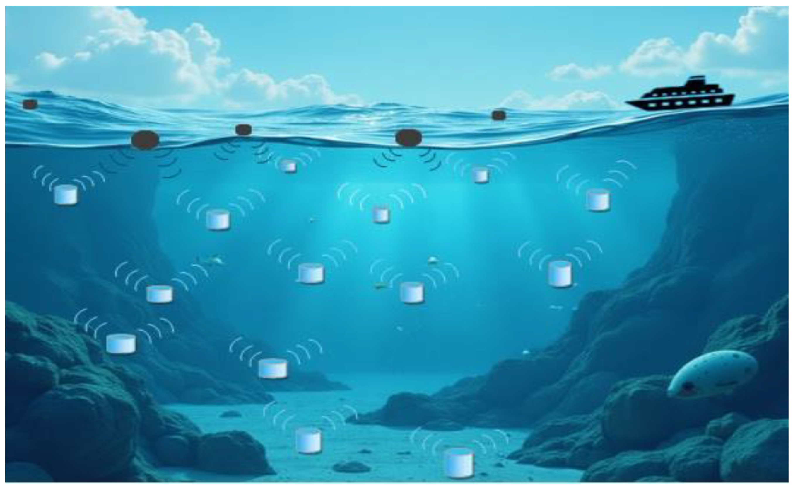
5. Proposed Reliable, Energy Optimized and Void Aware Routing Protocol

This research study proposes the implementation of a clustering-based routing protocol to reinforce network performance by cutting down the incidence of void issues and efficient energy utilization by balancing the energy usage among nodes. In this aspect, the nodes are positioned strategically within the underwater region.

5.1. Underwater Network Model Assumptions

The underwater network is assumed to be a 3D model. The networking elements are based on surface sink nodes (SSNs) and multiple acoustic sensor nodes (ASNs). The SSNs are outfitted with both RF modems and acoustic modems for onshore and underwater communication. However, the ASNs are only capable of acoustic communication with each other and the SSNs. The ASNs have been installed with a buoyancy control system that enables each ASN to maintain a specific depth within each layer [32]. The ASNs at each layer can move with the flow of water at a velocity ranging from 1 to 3 m per second. Vertically, an ASN may have a slight difference in depth, which is typically considered insignificant [44].

The battery life of SSNs is infinite but the battery life of every ASN is finite. Once depleted, ASNs are unable to sense, process, transmit, or receive. To conserve ASN and cluster head’s energy, the algorithm runs on sink nodes, leveraging their superior computational capacity and resources. SSNs use their global view of the network topology to make optimal routing decisions, effectively resolving void issues and enhancing data delivery reliability. The sink nodes disseminate routing decisions through control messages, which are received by cluster heads and shared with member nodes. Periodic beaconing ensures network synchronization while minimizing unnecessary overhead.

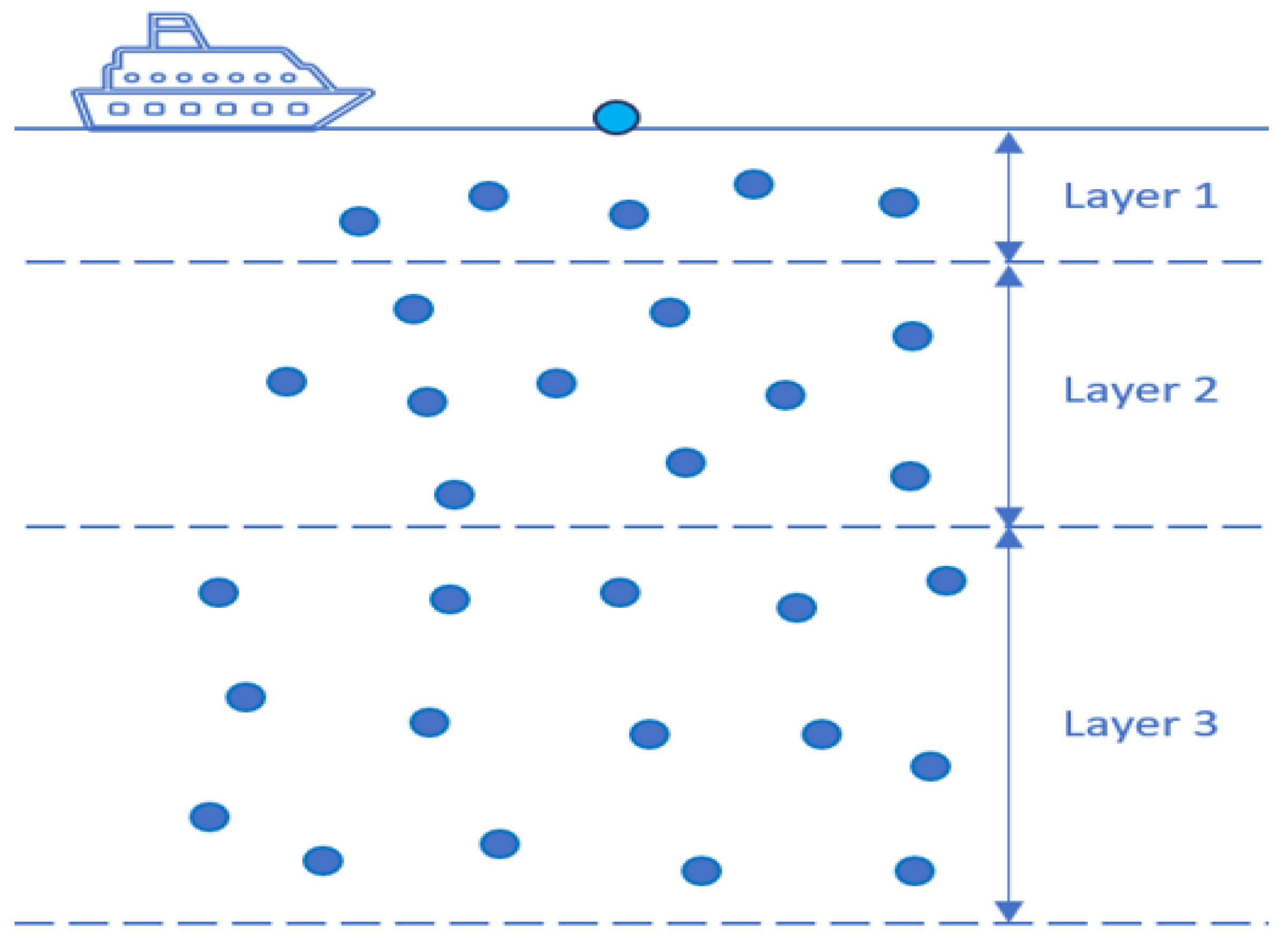
5.2. Strategic Deployment of Sensor Nodes

The 3D UASN network model is adopted from the research conducted in [23], where the underwater environment is segmented into unequal virtual layers. The first layer which is closest to the SSN has the smallest width, whereas the widths of the remaining layers increased with an arithmetic progression. The uniform distribution of ASNs in each unequal layer can increase the chances of sparser deployment in the widest layer, which triggers the possibility of void area occurrence [23,45,46].

For example, as per the deployment of ASNs considered in [47], the total sum of ASNs deployed in each layer is 100, and the volume (in cubic meters) of the first layer is 500 × 500 × 50 which is equivalent to 12,500,000, whereas the volume (in cubic meters) for the fifth layer is 500 × 500 × 150, which is equivalent to 37,500,000. There is a massive difference between the volumes of two distinctive layers. This massive difference affects the sparsity of the ASN deployment in each layer.

Consequently, there is a greater likelihood of void regions in the network. The designed routing protocol may not be suitable to be deployed in underwater monitoring regions having higher depths. Since there is no mechanism provided for controlling the void issue, the ASNs are high priced; therefore, strategically placing them in the submerged region will be favorable. The mathematical expression given below can be used to obtain the number of ASNs to be placed in each layer based on the width while keeping the ASN density constant.

$${\mathsf{{\rm N}}}_{\mathrm{\aleph }}={\mathrm{A}\mathrm{S}\mathrm{N}}_{\mathrm{d}}\times {\mathsf{\varpi }}_{\mathrm{\aleph }}$$

(14)

where ${\mathsf{{\rm N}}}_{\mathrm{\aleph }}$ is the total number of ASNs to be deployed in layer $\mathrm{\aleph }$, ${\mathrm{A}\mathrm{S}\mathrm{N}}_{\mathrm{d}}$ is the desired ASN density (nodes per unit width) and ${\mathsf{\varpi }}_{\mathrm{\aleph }}$ is the width of the layer $\mathrm{\aleph }$. Equation (14) ensures that the ASN density remains constant across all layers. The ASN density can be determined through Equation (15) by dividing the total sum of ASNs (${\mathrm{A}\mathrm{S}\mathrm{N}}_{\mathrm{T}}$) by the total width of the underwater networking region (${\mathsf{\varpi }}_{\mathrm{T}}$).

$${\mathrm{A}\mathrm{S}\mathrm{N}}_{\mathrm{d}}={\displaystyle \frac{{\mathrm{A}\mathrm{S}\mathrm{N}}_{\mathrm{T}}}{{\mathsf{\varpi }}_{\mathrm{T}}}}$$

(15)

To maintain uniform node density across all the layers, the number of ASNs to be deployed can be strategically placed in proportion to the width of the layer. This ensures that the ASNs density remains constant across all layers at the time of initial deployment. For instance, if the ${\mathsf{\varpi }}_1=100 \mathrm{m},{\mathsf{\varpi }}_2=150 \mathrm{m}$, ${\mathsf{\varpi }}_3=200 \mathrm{m},{\mathsf{\varpi }}_4=250 \mathrm{m}$, and ${\mathsf{\varpi }}_5=300 \mathrm{m},$ then the total number of ASNs to be deployed in each layer will be ${\mathsf{{\rm N}}}_1$ = 100 ASNs, ${\mathsf{{\rm N}}}_2$ = 150 ASNs, ${\mathsf{{\rm N}}}_3$ = 200 ASNs, ${\mathsf{{\rm N}}}_4$ = 250 ASNs, and ${\mathsf{{\rm N}}}_5$ = 300 ASNs. By doing so, each layer will have the same node density of one node per meter of width, ensuring uniform sparsity across all layers, which reduces the occurrence of the void region in the underwater networking region: for instance, as illustrated in Figure 3.

5.3. Information Dissemination

Since the ASNs are uninformed about the status of other neighboring ASNs; therefore, they initiate a Hello_Message containing their ID, residual energy, layer number, and depth information. The ASNs having built-in depth measuring gauges help in determining their depth values. Let us assume that n represents the total number of horizontal layers, beginning from the surface of the ocean. ${\mathsf{\varpi }}_{\mathrm{\aleph }}$ represents the width of the $\mathrm{\aleph }$th layer, while Ln represents the total depth of the nth layer. Each ASN can compute its layer identification using the following equation [47].

$${\mathrm{L}}_{\mathrm{n}}=\sum _{\mathrm{i}=1}^{\mathrm{n}}{\mathsf{\varpi }}_{\mathrm{\aleph }}$$

(16)

The layer identification at a certain depth dt can be determined by each ASN using the expression given below [47].

$${\mathrm{L}}_{\mathrm{n}}\le {\mathrm{d}}_{\mathrm{n}}<{\mathrm{L}}_{\mathrm{n}+1}$$

(17)

The Received Signal Strength Indicator (RSSI) of Hello_Message serves as an indicator of separation between neighboring ASNs. Each ASN compiles a list of other ASNs in the immediate vicinity after receiving the Hello_Message. To avoid excessive delays, the timeout duration is kept constant, which is equivalent to the maximum delay (dm) in transmitting data between two adjacent ASNs.

$$\mathrm{d}\mathrm{m}={\displaystyle \frac{{\mathrm{R}}_{\mathrm{t}}}{\mathrm{v}}}$$

(18)

where ${\mathrm{R}}_{\mathrm{t}}$ and $\mathrm{v}$ are the maximum transmission limits of ASN and the speed of sound underwater, which is 1500 m/s [17,38,48].

5.4. Clustering Process

The cluster formation and selection of cluster heads play a considerable role in the UASN environment. The proposed clustering procedure dynamically clusters the ASNs and selects a suitable cluster head for each cluster. However, before clustering, the optimal number of clusters is challenging.

Optimal Sum of Clusters

The optimal number of clustering is essential to accomplish energy efficiency among ASNs. A higher number of clusters while maintaining an equivalent processing load on each cluster head will result in the formation of numerous smaller-sized clusters; however, the communication overhead will also be higher. So, the energy expenditure is higher. Conversely, a smaller number of clusters will result in many larger-sized clusters, where the ASNs that are located further apart require a higher amount of energy to send data packets to their associated cluster head. Therefore, to preserve energy among acoustic sensor nodes, it is essential to choose the optimal sum of clusters. Optimizing the number of clusters enhances the longevity of the network, increases energy efficiency, and improves scalability. The studies in [49,50,51] used the K-means clustering to determine the optimal sum of clusters. However, the K-means algorithm requires the user to choose the number of clusters (K) before the clustering process begins. Additionally, if the locations of the ASNs do not vary once they are clustered, the network topology is fixed, which can result in an imbalance in energy usage among ASNs and leads to reduced lifespan. Therefore, in this paper, Algorithm 1 is proposed for the optimal number of clusters. The optimal number of clusters (K) can be calculated below.

Algorithm 1: Optimal Cluster Formation

Input: 3 Dimensions of Underwater Networking Region and Transmission Range Output: Optimal Number of Clusters Formation

For each layer i in depth Dn Calculate the % of the CH needed in each layer Calculate the total number of CH need in each layer End for For each node i in each layer Assign node to the nearest cluster center End for

$$\mathrm{K}={\displaystyle \frac{3\mathrm{L}\mathrm{B}\mathrm{D}}{4\mathsf{\pi }{{\mathrm{R}}_{\mathrm{t}}}^3}}$$

(19)

Here, L, B, and D, are the length in the X, breadth in the Y, and depth in the Z directions. ${\mathrm{R}}_{\mathrm{t}}$ is the maximum transmission range of ASN. Soon after the calculation of the optimal sum of clusters (K) required to cover the networking region, the ASNs are grouped into K clusters based on their submerged positions. The total number of clusters in each layer ${\mathrm{C}}_{\mathrm{\aleph }}$ can be calculated using the following expression.

$${\mathsf{\eta }}_{\mathrm{\aleph }}={\displaystyle \frac{{\mathsf{\varpi }}_{\mathrm{\aleph }}}{\mathrm{D}}}$$

(20)

$${\mathrm{C}}_{\mathrm{\aleph }}=\mathrm{K}\ast {\mathsf{\eta }}_{\mathrm{\aleph }}$$

(21)

Here, ${\mathsf{\eta }}_{\mathrm{i}}$ is the percentage of cluster formation in layer $\mathrm{\aleph }$, and D is the total depth assumed for the networking region.

$${\mathrm{D}}_{\mathrm{i}}={\displaystyle \frac{1}{\mathrm{N}-1}}\sum _{\mathrm{j}\ne \mathrm{i}}{\displaystyle \frac{1}{{\mathrm{R}\mathrm{S}\mathrm{S}\mathrm{I}}_{\mathrm{i},\mathrm{j}}}}$$

(22)

The higher RSSI values indicate the closer proximity of an ASN to the neighboring ASNs.

Residual Energy of the ASN: The cluster head expends a significantly higher amount of energy as compared to other ASNs. An ASN may prematurely die from excessive energy expenditure if it is frequently chosen as the cluster head and the chances of void area occurrence increase. The ASN with higher residual energy is a potential candidate to be selected as a cluster head. However, to reduce the occurrence of void area issues, a specific energy threshold is established for every ASN. Since the ASNs have less remaining energy than the mean remaining energy of cluster ASNs, it is unlikely to be chosen as the cluster- head. Consequently, the void area issue can be avoided by adopting a rotation policy while keeping the ASNs functional for a longer duration. The normalized value for the residual energy (${\mathrm{e}}_{\mathrm{R}\mathrm{e}\mathrm{s}}$) of ASN i can be calculated as follows.

$${\mathrm{e}}_{\mathrm{R}\mathrm{e}\mathrm{s}}={\displaystyle \frac{{\mathrm{E}}_{\mathrm{R}\mathrm{e}\mathrm{s}}-{\mathrm{E}}_{\mathrm{m}\mathrm{i}\mathrm{n}}}{{\mathrm{E}}_{\mathrm{m}\mathrm{a}\mathrm{x}}-{\mathrm{E}}_{\mathrm{m}\mathrm{i}\mathrm{n}}}}$$

(23)

Here, ${\mathrm{E}}_{\mathrm{m}\mathrm{a}\mathrm{x}},{\mathrm{a}\mathrm{n}\mathrm{d}\mathrm{E}}_{\mathrm{m}\mathrm{i}\mathrm{n}}$ are the maximum and minimum residual energy of all ASNs in the cluster. To select the optimal cluster head, we need a combined metric that considers both criteria. Algorithm 2 is proposed for the selection of Best Cluster Head. The combined metric best cluster head (BCH) for any ASN can be formulated as

$$\mathrm{B}\mathrm{C}\mathrm{H}=\mathsf{\alpha }{\mathrm{D}}_{\mathrm{i}}+\mathsf{\beta }\left({1-\mathrm{e}}_{\mathrm{R}\mathrm{e}\mathrm{s}}\right)$$

(24)

Here, α and β are the weighted parameters. The ASN having the highest BCH values in comparison to the other ASNs in a cluster will declare itself as a cluster head node by broadcasting a declared message. The ASNs respond to the declaration message by sending an acknowledgment message and agree to participate in the cluster as a member ASN.

Algorithm 2: Cluster Head Selection

Input: Optimal Number of Clusters Formation Output: Cluster Head Selection

For each cluster i in each layer For each node i in cluster Calculate the RSSI of node j Compare the residual energy of node j End For Calculate the best cluster head value If best cluster head value < Best Score Best cluster head value = Node_i End if End for

5.5. Routing Path Discovery Process

The cluster heads maintain a routing table that possesses the information of the nearby cluster heads by sending a beacon message. To reduce the overhead messaging, the transmission range of cluster heads is limited. Additionally, these beacon messages will only be received by the neighboring cluster heads that reside in the cluster head transmission range.

The beacon message contains the ASN ID, residual energy, depth value, and neighboring cluster head value. The routing path will be discovered based on the cost function given below.

$$\mathrm{R}\mathrm{P}=\mathsf{\delta }\left({\displaystyle \frac{{\mathrm{E}}_{\mathrm{R}\mathrm{E}\mathrm{S}}}{{\mathrm{E}}_{\mathrm{I}\mathrm{N}\mathrm{I}}}}\right)+\mathsf{\epsilon }\left(1-{\displaystyle \frac{{\mathrm{D}}_{\mathrm{C}\mathrm{H}}}{\mathrm{D}}}\right)+\mathsf{\rho }\left({\displaystyle \frac{{\mathrm{N}}_{\mathrm{C}\mathrm{H}}}{{\mathrm{T}}_{\mathrm{C}\mathrm{H}}}}\right)+{\mathsf{\sigma }\mathrm{L}}_{\mathrm{Q}}$$

(25)

where $\mathsf{\delta }+\mathsf{\epsilon }+\mathsf{\rho }+\mathsf{\sigma }=1$. ERES and EINI are the residual energy and initial energy of the cluster head, respectively. ${\mathrm{D}}_{\mathrm{C}\mathrm{H}}$ is the current depth value of the cluster head. ${\mathrm{N}}_{\mathrm{C}\mathrm{H}}$ and ${\mathrm{T}}_{\mathrm{C}\mathrm{H}}$ are the neighboring cluster heads and total cluster heads, respectively. LQ is the link quality of the cluster head. The cost function given in Equation (25) comprises the cluster head’s energy level, which indicates that the cluster head selection for the routing path having the higher residual energy will minimize the chances of early exhaustion of the network.

The depth parameter of the cluster head is also inducted in the cost function. The reason for introducing the depth parameter of the cluster head into the cost function is to preserve the energy of the node by reducing the chances of route selection being farther from the SSN. Furthermore, the neighboring cluster heads of the node are also considered as one of the factors of the cost function to lower the likelihood of void node problems, maintain network connectivity, and improve the packet delivery ratio. Also, the link quality is taken into consideration for calculating the cost function to make sure that the selected link is healthy enough to send data packets. The ASN having the maximum value of the cost function is the optimal choice for the next forwarder node among all the available neighboring cluster heads. Algorithm 3 is proposed for the reliable, energy optimized and void aware routing discovery.

Algorithm 3: Reliable, Energy Optimized and Void Aware Route Discovery

Input: Cluster Heads, Source Node Output: Optimal Routing Path Discovery

Initialize random node as source node. While the surface sink node is not found For each node i Calculate the routing path (RP) If RP > Best RP Best RP = RP Best neighbor = neighbor End If End For If the surface sink node is in the neighbor Send data directly to the surface sink nodes End if If no neighbor is found If waiting round > 2 then Drop packet End if Else Generate routing path End if End while

6. Simulation Environment

This section is bifurcated into simulation parameters and performance metrics.

6.1. Simulation Parameters

The simulations are conducted within a 3D underwater region, measuring 10 km × 10 km × 10 km. The sum of acoustic sensor nodes deployed in this environment varied between 100 and 500, which was distributed randomly yet strategically to ensure comprehensive coverage of the region. These acoustic sensor nodes are considered homogenous with an initial energy of 100 joules and a communication range of 2000 m. To facilitate communication, nine surface sink nodes are affixed on the water surface equidistant from each other to optimize data collection. The acoustic sensor nodes, subject to water current dynamics, exhibit horizontal mobility with the water flow at speeds ranging from 1 to 3 m per second. However, they are inhibited from abandoning the networking region. The data payload size is fixed to 200 bytes. A TDMA-based approach is assumed to handle potential packet collision and ensure efficient communication between nodes. This prevents simultaneous transmissions, thus avoiding interference and collisions regardless of node density. The packet transmission rate is influenced by the channel parameters, specifically the bandwidth (4 kHz) and channel bit rate (10 kbps), which define the theoretical data-handling capacity of the network. These simulation settings related to network dimensions, sinks, acoustic sensor nodes, and their movement within the defined region allowed the study of various performance metrics.

6.2. Performance Metrics

This subsection highlights the performance metrics of our proposed routing protocol as follows.

Packet Delivery Ratio (PDR): The packet delivery ratio is a way to measure the reliability of the network and can be defined as the ratio of total number of data packets positively received by the surface sink nodes to the total number of data packets transmitted by the source node. A higher PDR indicates better network performance in terms of reliability. Mathematically, PDR can be calculated as

$$\mathrm{P}\mathrm{D}\mathrm{R}=\left({\displaystyle \frac{\mathrm{P}\mathrm{a}\mathrm{c}\mathrm{k}\mathrm{e}\mathrm{t}\mathrm{s} \mathrm{r}\mathrm{e}\mathrm{c}\mathrm{e}\mathrm{i}\mathrm{v}\mathrm{e}\mathrm{d} \mathrm{b}\mathrm{y} \mathrm{s}\mathrm{i}\mathrm{n}\mathrm{k}}{\mathrm{P}\mathrm{a}\mathrm{c}\mathrm{k}\mathrm{e}\mathrm{t} \mathrm{t}\mathrm{r}\mathrm{a}\mathrm{n}\mathrm{s}\mathrm{m}\mathrm{i}\mathrm{t}\mathrm{t}\mathrm{e}\mathrm{d} \mathrm{b}\mathrm{y} \mathrm{s}\mathrm{o}\mathrm{u}\mathrm{r}\mathrm{c}\mathrm{e}}}\right)\times 100$$

(26)

Average Energy Consumption (AEC): Average energy consumption (AEC) represents the amount of energy utilized by the sensor nodes during the network operation. It can be defined by taking the difference between the initial energy (Einitial) and the remaining energy (Eresidual) of all the sensor nodes and dividing it by the total number of sensor nodes (N). Mathematically, it can be calculated as

$$\mathrm{A}\mathrm{E}\mathrm{C}={\displaystyle \frac{\sum _{\mathrm{i}=1}^{\mathrm{N}}\left({\mathrm{E}}_{\mathrm{i}\mathrm{n}\mathrm{i}\mathrm{t}\mathrm{i}\mathrm{a}\mathrm{l},\mathrm{i}}-{\mathrm{E}}_{\mathrm{r}\mathrm{e}\mathrm{s}\mathrm{i}\mathrm{d}\mathrm{u}\mathrm{a}\mathrm{l}},\mathrm{i}\right)}{\mathrm{N}}}$$

(27)

Average End-to-End Delay (AE2ED): Average end-to-end delay involves measuring the time it takes a data packet (P) to successfully travel from the source node ${(\mathrm{T}}_{\mathrm{s}\mathrm{e}\mathrm{n}\mathrm{d}})$ to the sink node (${\mathrm{T}}_{\mathrm{a}\mathrm{r}\mathrm{r}\mathrm{i}\mathrm{v}\mathrm{a}\mathrm{l}}$). It includes transmission delays, propagation delays, processing delays, and queuing delays. Mathematically, it can be calculated as

$$\mathrm{A}\mathrm{E}2\mathrm{E}\mathrm{D}={\displaystyle \frac{\sum _{\mathrm{i}=1}^{\mathrm{P}}\left({\mathrm{T}}_{\mathrm{a}\mathrm{r}\mathrm{r}\mathrm{i}\mathrm{v}\mathrm{a}\mathrm{l},\mathrm{i}}-{\mathrm{T}}_{\mathrm{s}\mathrm{e}\mathrm{n}\mathrm{d},\mathrm{i}}\right)}{\mathrm{P}}}$$

(28)

Dead Nodes (DN): Dead nodes (DNs) refer to the number of nodes that have exhausted their energy and can no longer participate in network operations. Dead nodes are crucial for understanding the longevity and sustainability of the network. Mathematically, they can be calculated as the difference of the deployed nodes (N) to the operational nodes (ON):

$$\mathrm{D}\mathrm{N}=\mathrm{N}-\mathrm{O}\mathrm{N}$$

(29)

Total Energy Consumption (TEC): Total energy consumption is the absolute energy used by all the sensor nodes in the network. It is based on the transmission energy, reception energy, and the energy consumed by all the nodes remaining in the idle state. This work only considered the energy consumed during activities such as transmission and reception.

$$\mathrm{T}\mathrm{E}\mathrm{C}={\sum }_{\mathrm{i}=1}^{\mathrm{N}}({\mathrm{E}}_{\mathrm{t}\mathrm{x}}^{\mathrm{i}}+{\mathrm{E}}_{\mathrm{r}\mathrm{x}}^{\mathrm{i}})$$

(30)

Network Throughput (NT): Network throughput is defined as the total amount of data successfully delivered to the sink nodes per unit of time. It is measured in kilobits per second. Mathematically, it can be calculated as

$$\mathrm{N}\mathrm{T}=\left({\displaystyle \frac{\mathrm{P}\mathrm{a}\mathrm{c}\mathrm{k}\mathrm{e}\mathrm{t}\mathrm{s} \mathrm{r}\mathrm{e}\mathrm{c}\mathrm{e}\mathrm{i}\mathrm{v}\mathrm{e}\mathrm{d} \mathrm{b}\mathrm{y} \mathrm{s}\mathrm{i}\mathrm{n}\mathrm{k}}{\mathrm{T}\mathrm{o}\mathrm{t}\mathrm{a}\mathrm{l} \mathrm{T}\mathrm{i}\mathrm{m}\mathrm{e}}}\right)\times 1000$$

(31)

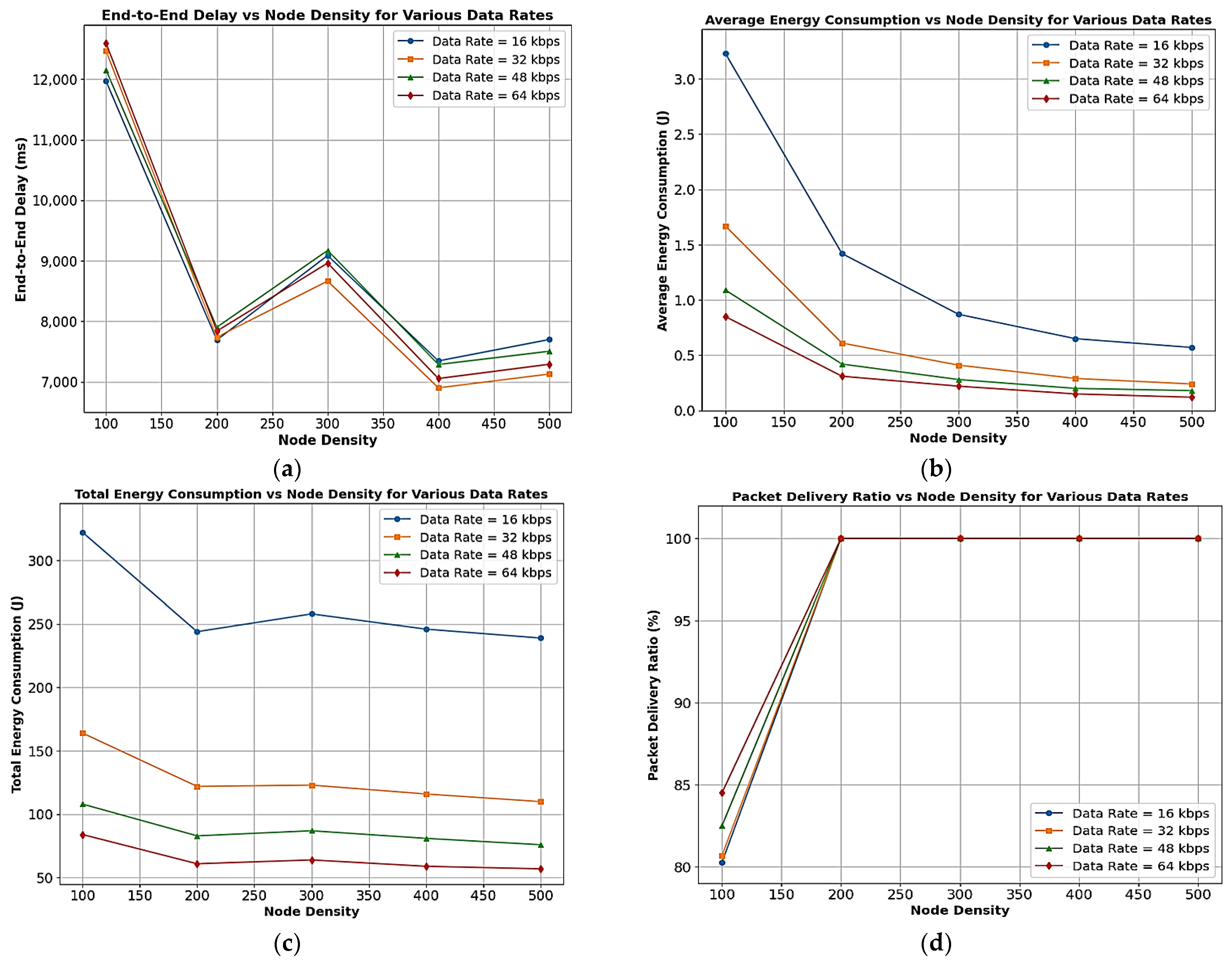
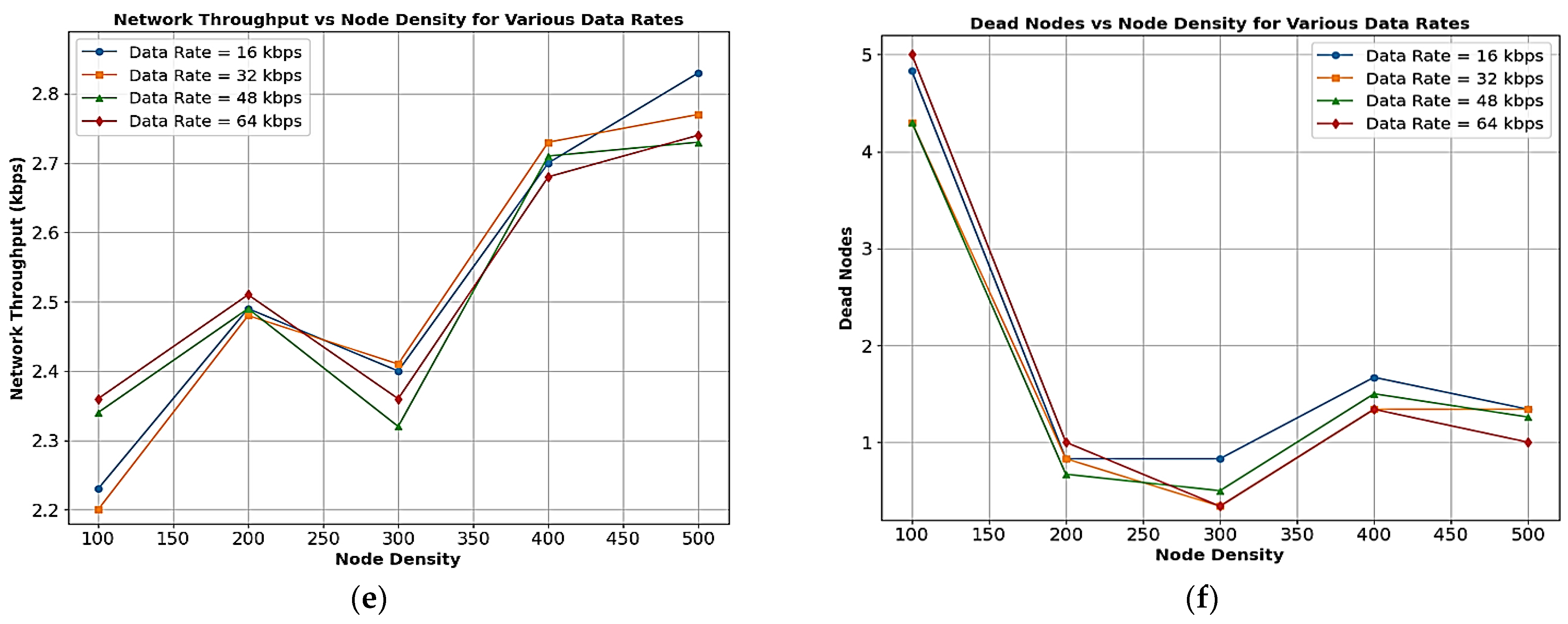
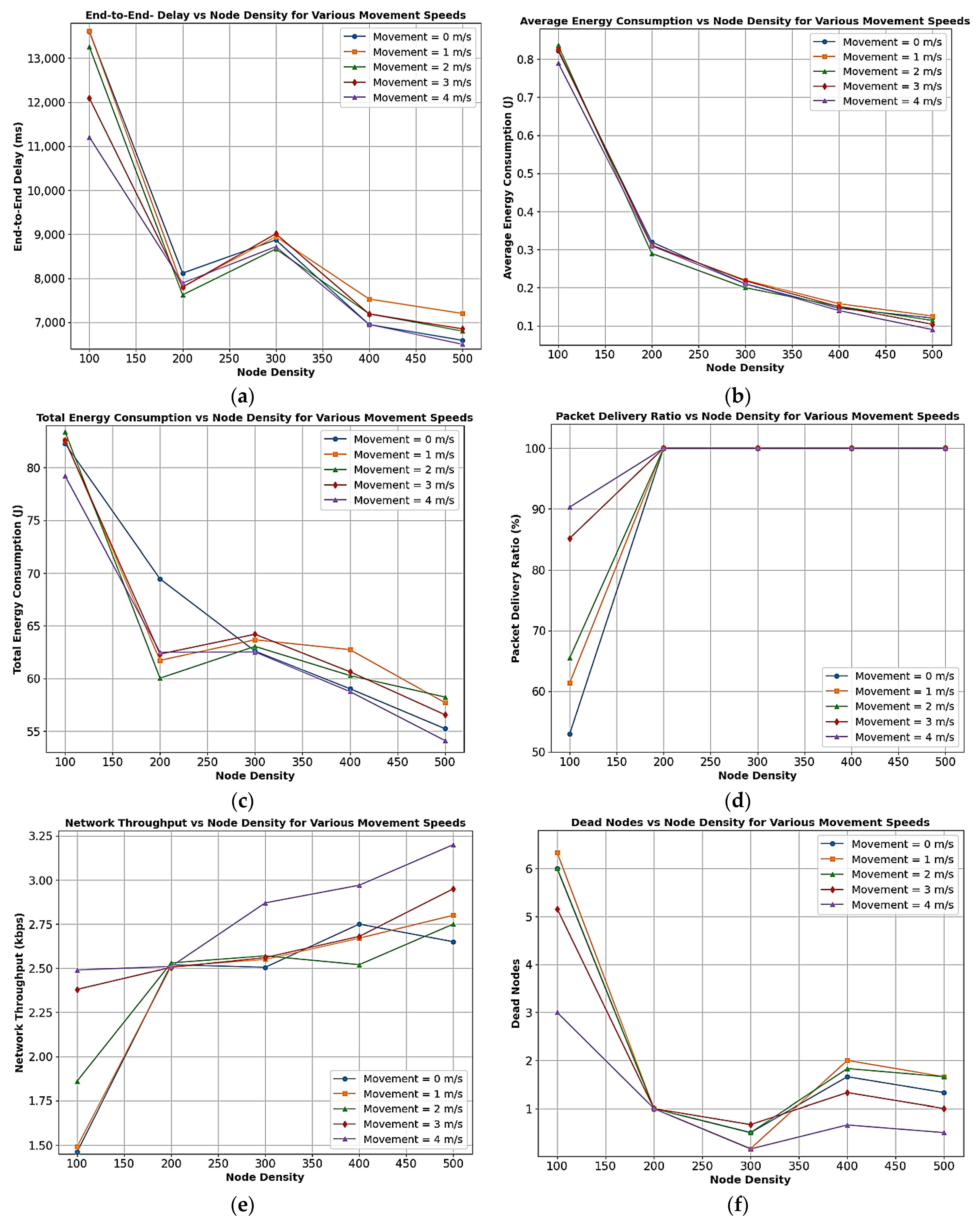
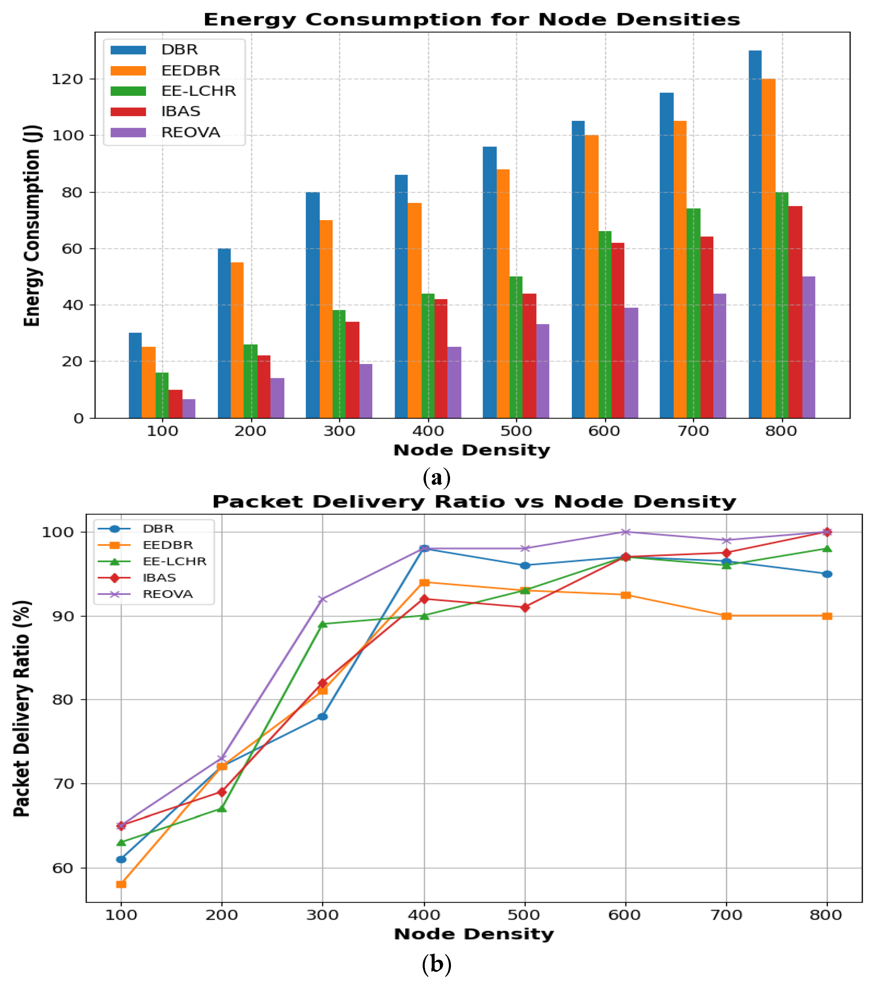
7. Results and Discussion

This section investigates how different network parameters influence the performance of our proposed routing protocol. The analysis focuses on examining the impact of each parameter individually by altering one at a time while keeping the remaining network parameters unchanged.

Effect of Data Rates: To examine the effect of data rates on the network performance, a series of simulations with fixed data rates of 16, 32, 48, and 64 kbps has been performed. The results from these simulations are illustrated in Figure 4 and explained below.

Figure 4a illustrates the end-to-end delay as data rates and node density varied. The end-to-end delay declines with an increase in data rates and node density because, with the higher data rates, the packets are transmitted faster across the network, reducing the time span for data to travel from the source to the destination. Additionally, the higher data rates allow the network to handle more data in a short time, reducing congestion. Consequently, the data packet experiences fewer delays waiting for transmission, which leads to quicker end-to-end delay. Furthermore, with higher node density, there are more available paths for routing data, increasing the likelihood of finding shorter and faster routes. More nodes also improve connectivity, minimizing the likelihood of experiencing void regions and further lowering the delays.

Figure 4b illustrates the average energy consumption by nodes as the data rates and node density varied. The observed reduction in average energy consumption by nodes as data rates and node density increase can be explained by several factors. Firstly, higher data rates enable faster packet transmission, thereby reducing the time nodes spend in transmission mode, which directly lowers energy usage, as energy consumption is directly related to the duration of transmission. Secondly, with the greater node density, the data packet can be transmitted over a shorter distance, which leads to lower power requirements for communication, further reducing energy usage. Lastly, the combination of higher data rates and increased node density improves overall network reliability, decreasing the likelihood of packet loss and consequently reducing the need for energy-intensive retransmission.

Figure 4c illustrates the total energy consumption by the network as the data rates and node density varied. There is a slight decline in TEC across the network as the data rates and node density increase due to the usage of higher data rates, which improves the energy efficiency by allowing rapid data transmission, thereby reducing the time spent in transmission mode. This leads to overall lower energy usage.

Additionally, the higher node density enhances network reliability by offering a higher number of available paths for data transmission, which lowers the possibility of packet loss and/or retransmission. Also, the implementation of void-aware route selection ensures that data are directed through energy-efficient routes, avoiding sparsely populated areas and resulting in lower energy consumption.

Figure 4d illustrates the packet delivery ratio as the data rates and node density varied. The PDR increases with the rise in data rates and node density. The cause for improved PDR is the higher node density, which provides more available routes to choose an optimal path for data transmission, significantly reducing the possibility of experiencing void regions with sparse or no node coverage. Void-aware routing ensures that data are directed through the most efficient path, bypassing all problematic regions, which enhances the overall PDR. Furthermore, the use of higher data rates speeds up the transmission, minimizing packet loss and further improving network reliability.

Figure 4e illustrates the network throughput as the data rates and node density varied. There is an increase in NT with rising data rates and node density, despite a slight dip at 300 nodes. Higher data rates enable faster data transmission, allowing the network to process larger volumes of data in less time, thus improving the network throughput. Furthermore, as the node density increases, connectivity improves, which reduces the congestion and increases data flow. The slight dip at 300 nodes may result from temporary network congestion or increased collision due to suboptimal routing. However, as the node count reaches 400 and 500, the network recovers, benefiting from better connectivity and more efficient path selection that enhances the network throughput. Also, with the higher node density, the network can distribute the communication load more evenly. This reduces the burden on individual nodes and prevents congestion at a specific point, which leads to smoother data flow and improved network throughput.

Figure 4f illustrates the sum of dead nodes as the data rates and node density varied. There is a significant reduction in the sum of DNs as the node density increases. At lower node density, fewer nodes are available to relay the data packets, which results in longer transmission distances and higher energy consumed per node, which leads to premature node death. As the node density increases, the average distance between nodes decreases, which allows more energy-efficient communication. Additionally, with the increase in the data rates, the number of DN reduces as faster data transmission reduces the time spent in transmission mode. This enhanced energy efficiency at higher data rates, particularly in less dense networks, further contributes to the observed reduction in dead nodes.

Effect of Node Movement with Various Speeds: To examine the effect of node movement with different speeds on network performance, we carried out a series of simulations with fixed node movement speeds of static (fixed nodes), 1, 2, 3, and 4 m/s. The results from these simulations are illustrated in Figure 5 and explained in the paragraphs below.

Figure 5a illustrates the end-to-end delay as the node movement (0 to 4 m/s) and node density varied. There is a significant decrease in end-to-end delay as the node density increases particularly in the range of 100 to 200 nodes with a gradual decline after this point. This reduction can be attributed to the higher availability of communication paths in denser networks, which shortens the average transmission distance between nodes, thereby dropping the sum of hops required to deliver the data packets to the destination. Given the relatively slow propagation speed of sound in underwater environments, shorter transmission distances significantly reduce propagation delay, hence improving the overall network performance. Furthermore, the impact of node movement speed on the routing stability becomes evident at higher speeds, particularly at 3 and 4 m/s, where frequent changes in topology lead to route discovery delays and link breakages, slightly increasing the end-to-end delay. In contrast, at lower movement speeds, particularly 0 m/s and 1 m/s, the network experiences fewer disruptions, resulting in more stable and reliable routing.

Figure 5b illustrates the average energy utilization per node as the node movement (0 to 4 m/s) and node density varied. Although the AEC per node has decreased significantly, the node movement has a relatively minor effect on the overall trend of the average energy utilization. As the node density rises, the network can maintain efficient routing, even with nodes moving at faster speeds. The high density allows for a larger number of potential nodes, ensuring that disruptions caused by node mobility are quickly compensated by alternative routing paths. At lower node density, faster movement speed may cause a minor raise in energy expenditure as fewer adjacent nodes are available for routing and need frequency route recalculations. However, in higher density, this variation in energy consumption across different movement speeds becomes negligible as the network’s ability to adapt to topology changes balances the potential energy cost.

Figure 5c illustrates the total energy consumption as the node movement (0 m/s to 4 m/s) and node density varied. As node density increases, the total energy expenditure decreases. As node density rises, the proximity of neighboring nodes reduces the transmission distance, leading to lower energy utilization. This not only optimized energy efficiency but also enhances the reliability of the network by providing more alternative routing options, which helps to mitigate the risks associated with void areas. In lower node density, the void region forces nodes to send them over greater distances, which increases energy usage. However, higher node density reduces the possibility of encountering void holes, facilitating more energy-efficient routing. Furthermore, while node movement speed introduces some variation in energy consumption, its impact diminishes as node density increases.

Figure 5d illustrates the packet delivery ratio as the node movement (0 m/s to 4 m/s) and node density varied. The PDR increases with the increase in the node movement as well as node density. As the node density increases, the network becomes more robust due to the higher availability of neighboring nodes. The greater node availability reduces the chances of void regions without node availability, which could lead to packet loss. Also, mobile nodes increase more routing opportunities as they move, increasing the possibility of maintaining connectivity and finding alternate routes around void nodes. This adaptability allows the network to adjust its routing paths in real time, enhancing the probability that packets will reach their destination successfully. Both the node density and movement contribute to the observed 100% reliability in the PDR. By selecting routes with higher node availability, movement, and optimal link quality, the network minimizes the chances of packet loss, ensuring reliable packet delivery.

Figure 5e illustrates the network throughput as the node movement (0 m/s to 4 m/s) and node density varied. The graphical representation demonstrates a positive correlation between the NT and increased node density and movement speed. As node density increases, it improves the connectivity by reducing void regions and shortens the transmission distances, enhancing both energy efficiency and reliability. Additionally, moderate node movement (1 m/s to 3 m/s) provides more dynamic routing opportunities, which allow for adaptive path selection that mitigates void issues and maintains high reliability. At higher node movement speeds, with the NT elevated, the network stability can be compromised due to rapid topology changes. The combined effect of these factors highlights how void-aware, energy-efficient routing optimizes throughput while maintaining reliability in dynamic underwater environments.

Figure 5f illustrates the number of dead nodes as the node movement (0 m/s to 4 m/s) and node density varied. As the node density increases, the number of dead nodes decreases significantly. This can be due to improved connectivity and reduced void regions. At higher node density (400 nodes to 500 nodes) and with increased node movement speeds, the network maintains stability due to an increased number of alternative paths, which mitigates the impact of topological changes caused by faster-moving nodes. Although faster node movement speeds can introduce instability, the higher node density compensates for it by ensuring continuous route availability, leading to minimal node failures.

Effect of Payload: To examine the effect of data payload on network performance, we carried out a series of simulations with data payloads of 200, 300, 400, and 500 bytes. The results from these simulations are shown in Figure 6 and explained in the paragraphs below.

Figure 6a illustrates the end-to-end delay as payload (200 bytes to 500 bytes) and node density varied. The graph indicates a significant drop in end-to-end delay as the node density increases, which is because of improved network connectivity at higher node densities. The nodes having more neighboring nodes in their transmission range reduce the number of hops required for data transmission. Fewer hops lead to lower overall transmission delays. Larger payload sizes take more time to transmit due to the increased data volume, resulting in slightly higher delays. However, in denser networks, the negative impact of larger payload size is mitigated by the availability of more efficient routes, which compensates for the longer transmission delays. This highlights that higher node densities not only reduce delay but also make the network more robust to the challenges posed by larger data packets. Consequently, the network maintains lower delays even with heavier data traffic, optimizing the overall performance.

Figure 6b illustrates the average energy expenditure per node as the payload (200 bytes to 500 bytes) and node density varied. The mean energy expenditure decreases as node density increases, which can be explained by the shorter communication paths available in denser networks. With more nodes in the network, data packets require fewer hops to reach their destination, reducing the energy expended by each node during transmission. Smaller payloads such as 200 bytes consume less energy, since they require less transmission time. Larger payloads such as 500 bytes, while consuming more energy initially due to their size, benefit from the efficiency of higher node densities, which compensates for the additional energy costs. The decrease in energy consumption is more obvious due to densely populated regions as the availability of alternative routes helps avoid energy-intensive long-distance transmissions.

Figure 6c illustrates the total energy expenditure as the payload and node density varied. The total energy consumption graph reflects a downward trend as node density increases, like the average energy consumption. A larger payload size such as 500 bytes results in higher total energy consumption. However, as the node density increases, the efficiency of the network improves due to a shorter communication path, leading to a decrease in total energy consumption. Denser networks reduce void regions where nodes would waste energy searching for available routes.

Figure 6d illustrates the packet delivery ratio as the payload and node density varied. The packet delivery ratio increases rapidly as the node density rises. This is because the higher node density provides more robust connectivity and different paths for data transmission, which helps mitigate the effects of packet loss due to void regions. Also, with larger payloads like 500 bytes, which could increase the chance of packet loss due to longer transmission times, the packet delivery ratio remains high in dense networks. The graph highlights that network density plays a more critical role in ensuring reliable data transmission than payload size, as a dense network can handle lager data volumes without compromising packet delivery.

Figure 6e illustrates the network throughput as the payload and node density varied. The network throughput improves as node density increases with larger payload sizes, such as 500 bytes, consistently achieving higher network throughput compared to smaller payload sizes. This is because of the enhanced efficiency of data transmission in larger payloads as they allow more data to be sent per packet, reducing the overall number of packets needed for transmission. Additionally, larger payloads reduce the ratio of packet overhead to the actual data transmitted. Also, higher node density and route selection based on neighboring nodes provide more robust networks with more available routes, which reduces the possibility of void regions.

Figure 6f illustrates the number of dead nodes as payload (200 bytes to 500 bytes) and node density varied. The number of dead nodes decreases as node density increases. In sparse networks, nodes are more likely to deplete their energy rapidly, especially when transmitting larger-sized payloads such as 500 bytes, due to the longer distances required for communication and fewer available nodes. Larger payloads can lead to higher energy consumption, which can lead to a higher number of dead nodes prematurely. However, as node density increases, the network becomes more energy efficient and prolongs their network lifetime.

Network Performance Comparative Analysis: This proposed research work provides a network performance comparison with some of the existing state-of-the-art routing protocols. The network performance of our proposed routing strategy, REOVA, is compared with DBR [28], EE-LCHR [38], EEDBR [48], and IBAS [52].

The network performance of our proposed routing protocol REOVA is compared with the routing protocols based on three performance metrics, e.g., energy consumption, packet delivery ratio, and end-to-end delay. The total number of considered nodes is 100 with a difference of 100 nodes to the maximum number of nodes of 800. The 3D underwater network boundaries are defined as 1000 m on each X, Y, and Z plane. Each node has an initial energy of 10,000 µJ, with the transmission mode power consumption, and it receives mode power consumption of 2 µJ and 0.5 µJ, respectively. The maximum transmission distance, the packet size, and simulations are defined as 250 m, 50 bytes, and 50, respectively. The simulation parameters are defined to ensure fair comparison as in [38].

Figure 7a illustrates the comparison of our proposed routing protocol with some existing routing protocols in terms of energy consumption (EC). The EC of our proposed protocol is much less than that of other routing protocols. DBR consumed the highest energy. The energy expenditure of EEDBR is much higher as compared to all the other routing protocols because data packets often either travel longer paths or repeatedly burden specific nodes, which leads to higher energy tax.

The EE-LCHR used a residual energy-based cluster head rotation mechanism. However, its energy consumption is also higher than IBAS and the proposed scheme. The IBAS protocol election of a cluster head on the fitness function emphasized direct communication from the cluster head to the sink node and never considered the communication path quality and nearby node to preserve energy.

Our proposed routing protocol is significantly efficient in terms of energy usage due to the proposed combination of strategic node deployment and the efficient selection of routing path based on residual energy, link quality, and neighboring cluster head node density, outperforming the other existing approaches.

Figure 7b illustrates the comparison of our proposed routing protocol with some existent routing protocols in terms of packet delivery ratio. The node densities in all the routing protocols, which are considered for the comparison of PDR, are the decisive factor in successfully routing data packets to their destination. The DBR and EEDBR are slightly less reliable in routing data packets to their destination due to the frequent selection of similar nodes for routing packets. This could lead to the early demise of such nodes and create larger gaps between nodes, which can disrupt communication. Likewise, in EE-LCHR and IBAS, the node deployment is random, which may create some regions densely populated and others sparsely populated. Additionally, the forwarding mechanism disregards the link quality and unconsidered the void areas before making routing decisions. Our proposed routing scheme ensures the selection efficient path selection and hence surpasses the remaining routing protocols even at the lesser node densities.

Figure 7c illustrates the comparison of our proposed routing protocol with some existing routing protocols in terms of end-to-end-delay. The DBR and EEDBR routing protocols suffer from the issue of void regions where no nodes are available to route the packet to the destination. This problem is significantly higher, especially in lesser node density networks, and causes longer end-to-end delay. The EE-LCHR and IBAS exhibit almost similar end-to-end-delay, which is the least among all the compared routing protocols. The end-to-end-delay experienced by our proposed routing protocol is significantly shorter than DBR and EEDBR; however, it is slightly longer than EE-LCHR and IBAS. Our proposed strategy is focused on transferring the data to the cluster head, having better link quality. In dynamic environments, the link stability swings rapidly, which leads to packet transmission to the nearest cluster head. This brings in a higher number of hop counts. Although the reliability increases, and energy is preserved, the end-to-end delay increases.

8. Conclusions

This research paper proposed a multi-hop routing protocol for Underwater Acoustic Sensor Networks. The study examines various existing routing protocols and addresses the triple challenges of reliability, energy conservation, and void hole mitigation. Through a novel way of strategic node deployment, optimal clustering, and void-aware routing path selection, our findings demonstrate a significant improvement in network efficiency, achieving reduced energy consumption while enhancing the packet delivery ratio. This study offers an energy-efficient and reliable UASN network, promoting sustainable oceanographic data collection and monitoring. The results suggest that our proposed methodology can contribute to prolonging the network lifespan of UASNs in challenging underwater environments, offering practical solutions for real-world applications where data timeliness is less critical. Future work may explore the improvement toward reducing the longer delays, which may significantly improve the network performance, especially for the applications where quicker transmissions are needed to make time-critical decisions.

References

1. Shah, S.M.; Sun, Z.; Zaman, K.; Hussain, A.; Ullah, I.; Ghadi, Y.Y.; Khan, M.A.; Nasimov, R. Advancements in Neighboring-Based Energy-Efficient Routing Protocol (NBEER) for Underwater Wireless Sensor Networks. Sensors 2023, 23, 6025. [Google Scholar] [CrossRef] [PubMed]
2. Shakila, R.; Paramasivan, B. An improvised optimization algorithm for submarine detection in underwater wireless sensor networks. Microsyst. Technol. 2024, 30, 185–196. [Google Scholar] [CrossRef]
3. Khan, A.; Khan, M.; Ahmed, S.; Iqbal, N.; Abd Rahman, M.A.; Abdul Karim, M.K.; Mustafa, M.S.; Yaakob, Y. EH-IRSP: Energy Harvesting Based Intelligent Relay Selection Protocol. IEEE Access 2021, 9, 64189–64199. [Google Scholar] [CrossRef]
4. Wibisono, A.; Piran, M.J.; Song, H.K.; Lee, B.M. A Survey on Unmanned Underwater Vehicles: Challenges, Enabling Technologies, and Future Research Directions. Sensors 2023, 23, 7321. [Google Scholar] [CrossRef]
5. Wang, Z.; Han, G.; Qin, H.; Zhang, S.; Sui, Y. An Energy-Aware and Void-Avoidable Routing Protocol for Underwater Sensor Networks. IEEE Access 2018, 6, 7792–7801. [Google Scholar] [CrossRef]
6. Khan, A.M.; Luque-Nieto, M.A.; Siddique, A.A. Underwater Efficient Data Routing: Clustering-Travel Salesman Protocol (CTSP). IEEE Access 2024, 12, 26428–26440. [Google Scholar] [CrossRef]
7. Khasawneh, A.M.; Kaiwartya, O.; Lloret, J.; Abuaddous, H.Y.; Abualigah, L.; Al Shinwan, M.; Al-Khasawneh, M.A.; Mahmoud, M.; Kharel, R. Green communication for underwater wireless sensor networks: Triangle metric based multi-layered routing protocol. Sensors 2020, 20, 7278. [Google Scholar] [CrossRef]
8. Gola, K.K. A Comprehensive Survey of Localization Schemes and Routing Protocols with Fault Tolerant Mechanism in UWSN- Recent Progress and Future Prospects; Springer: New York, NY, USA, 2024; ISBN 0123456789. [Google Scholar]
9. Mhemed, R.; Comeau, F.; Phillips, W.; Aslam, N. Void avoidance opportunistic routing protocol for underwater wireless sensor networks. Sensors 2021, 21, 1942. [Google Scholar] [CrossRef]
10. Tian, K.; Zhou, C.; Zhang, J. Improved LEACH Protocol Based on Underwater Energy Propagation Model, Parallel Transmission, and Replication Computing for Underwater Acoustic Sensor Networks. Sensors 2024, 24, 556. [Google Scholar] [CrossRef]
11. Yu, W.; Chen, Y.; Wan, L.; Zhang, X.; Zhu, P.; Xu, X. An Energy Optimization Clustering Scheme for Multi-Hop Underwater Acoustic Cooperative Sensor Networks. IEEE Access 2020, 8, 89171–89184. [Google Scholar] [CrossRef]
12. Nguyen, N.T.; Le, T.T.T.; Nguyen, H.H.; Voznak, M. Energy-efficient clustering multi-hop routing protocol in a UWSN. Sensors 2021, 21, 627. [Google Scholar] [CrossRef]
13. Latif, K.; Javaid, N.; Ullah, I.; Kaleem, Z.; Malik, Z.A.; Nguyen, L.D. Dieer: Delay-intolerant energy-efficient routing with sink mobility in underwater wireless sensor networks. Sensors 2020, 20, 3467. [Google Scholar] [CrossRef] [PubMed]
14. Joshi, S.; Anithaashri, T.P.; Rastogi, R.; Choudhary, G.; Dragoni, N. IEDA-HGEO: Improved Energy Efficient with Clustering-Based Data Aggregation and Transmission Protocol for Underwater Wireless Sensor Networks. Energies 2023, 16, 353. [Google Scholar] [CrossRef]
15. Xiao, X.; Huang, H. A clustering routing algorithm based on improved ant colony optimization algorithms for underwater wireless sensor networks. Algorithms 2020, 13, 250. [Google Scholar] [CrossRef]
16. Zhang, J.; Wang, X.; Wang, B.; Sun, W.; Du, H.; Zhao, Y. Energy-Efficient Data Transmission for Underwater Wireless Sensor Networks: A Novel Hierarchical Underwater Wireless Sensor Transmission Framework. Sensors 2023, 23, 5759. [Google Scholar] [CrossRef]
17. Karim, S.; Shaikh, F.K.; Aurangzeb, K.; Chowdhry, B.S.; Alhussein, M. Anchor Nodes Assisted Cluster-Based Routing Protocol for Reliable Data Transfer in Underwater Wireless Sensor Networks. IEEE Access 2021, 9, 36730–36747. [Google Scholar] [CrossRef]
18. Ganesh, N. Performance Evaluation of Depth Adjustment and Void Aware Pressure Routing (DA-VAPR) Protocol for Underwater Wireless Sensor Networks. Comput. J. 2020, 63, 193–202. [Google Scholar] [CrossRef]
19. Zhu, R.; Jiang, Q.; Huang, X.; Li, D.; Yang, Q. A Reinforcement-Learning-Based Opportunistic Routing Protocol for Energy-Efficient and Void-Avoided UASNs. IEEE Sens. J. 2022, 22, 13589–13601. [Google Scholar] [CrossRef]
20. Singh, B.; Gupta, B. An Energy Efficient Optimal Path Routing (EEOPR) for Void Avoidance in Underwater Acoustic Sensor Networks. Int. J. Comput. Netw. Inf. Secur. 2022, 14, 19–32. [Google Scholar] [CrossRef]
21. Jin, Z.; Zhao, Q.; Luo, Y. Routing Void Prediction and Repairing in AUV-Assisted Underwater Acoustic Sensor Networks. IEEE Access 2020, 8, 54200–54212. [Google Scholar] [CrossRef]
22. Yildiz, H.U. Joint Effects of Void Region Size and Sink Architecture on Underwater WSNs Lifetime. IEEE Sens. J. 2023, 23, 11046–11056. [Google Scholar] [CrossRef]
23. Deng, X.; Shi, L.; Li, Y.; Luo, L.; Zheng, L. A Void-Avoidable and Reliability-Based Opportunistic Energy Efficiency Routing for Mobile Sparse Underwater Acoustic Sensor Network. In Proceedings of the 2021 IEEE/ACIS 20th International Fall Conference on Computer and Information Science (ICIS Fall), Xi’an, China, 13–15 October 2021; pp. 269–274. [Google Scholar] [CrossRef]
24. Bouk, S.H.; Ahmed, S.H.; Park, K.J.; Eun, Y. EDOVE: Energy and depth variance-based opportunistic void avoidance scheme for underwater acoustic sensor networks. Sensors 2017, 17, 2212. [Google Scholar] [CrossRef]
25. Sher, A.; Khan, A.; Javaid, N.; Ahmed, S.H.; Aalsalem, M.Y.; Khan, W.Z. Void hole avoidance for reliable data delivery in IoT enabled underwater wireless sensor networks. Sensors 2018, 18, 3271. [Google Scholar] [CrossRef]
26. Gola, K.K.; Gupta, B. Underwater Acoustic Sensor Networks: An Energy Efficient and Void Avoidance Routing Based on Grey Wolf Optimization Algorithm. Arab. J. Sci. Eng. 2021, 46, 3939–3954. [Google Scholar] [CrossRef]
27. Coutinho, R.W.L.; Boukerche, A.; Vieira, L.F.M.; Loureiro, A.A.F. GEDAR: Geographic and opportunistic routing protocol with Depth Adjustment for mobile underwater sensor networks. In Proceedings of the 2014 IEEE International Conference on Communications (ICC), Sydney, NSW, Australia, 10–14 June 2014; pp. 251–256. [Google Scholar] [CrossRef]
28. Yan, H.; Shi, Z.J.; Cui, J.H. DBR: Depth-based routing for underwater sensor networks. In Proceedings of the 7th International IFIP-TC6 Networking Conference, Singapore, 5–9 May 2008; pp. 72–86. [Google Scholar] [CrossRef]
29. Noh, Y.; Lee, U.; Lee, S.; Wang, P.; Vieira, L.F.M.; Cui, J.H.; Gerla, M.; Kim, K. HydroCast: Pressure routing for underwater sensor networks. IEEE Trans. Veh. Technol. 2016, 65, 333–347. [Google Scholar] [CrossRef]
30. Barbeau, M.; Blouin, S.; Cervera, G.; Garcia-alfaro, J.; Barbeau, M.; Blouin, S.; Cervera, G.; Garcia-alfaro, J.; Kranakis, E. Location-free link state routing for underwater acoustic sensor networks. To cite this version: HAL Id: Hal-01263407 Location-free Link State Routing for Underwater Acoustic Sensor Networks. In Proceedings of the 2015 IEEE 28th Canadian Conference on Electrical and Computer Engineering (CCECE), Halifax, NS, Canada, 3–6 May 2016. [Google Scholar]
31. Ghoreyshi, S.M.; Shahrabi, A.; Boutaleb, T. An inherently void avoidance routing protocol for underwater sensor networks. In Proceedings of the 2015 International Symposium on Wireless Communication Systems (ISWCS), Brussels, Belgium, 25–28 August 2015; pp. 361–365. [Google Scholar] [CrossRef]
32. Khan, W.; Wang, H.; Anwar, M.S.; Ayaz, M.; Ahmad, S.; Ullah, I. A Multi-Layer Cluster Based Energy Efficient Routing Scheme for UWSNs. IEEE Access 2019, 7, 77398–77410. [Google Scholar] [CrossRef]
33. Karim, S.; Shaikh, F.K.; Chowdhry, B.S. Void Handling in Routing Protocols for Underwater Wireless Sensor Networks: A Quantitative Analysis. In Proceedings of the 2021 IEEE 18th International Conference on Smart Communities: Improving Quality of Life Using ICT, IoT and AI (HONET), Karachi, Pakistan, 11–13 October 2021; pp. 137–142. [Google Scholar] [CrossRef]
34. Noh, Y.; Lee, U.; Wang, P.; Choi, B.S.C.; Gerla, M. VAPR: Void-aware pressure routing for underwater sensor networks. IEEE Trans. Mob. Comput. 2013, 12, 895–908. [Google Scholar] [CrossRef]
35. Basagni, S.; Petrioli, C.; Petroccia, R.; Spaccini, D. CARP: A Channel-aware routing protocol for underwater acoustic wireless networks. Ad Hoc Netw. 2015, 34, 92–104. [Google Scholar] [CrossRef]
36. Rahman, M.A.; Lee, Y.; Koo, I. EECOR: An Energy-Efficient Cooperative Opportunistic Routing Protocol for Underwater Acoustic Sensor Networks. IEEE Access 2017, 5, 14119–14132. [Google Scholar] [CrossRef]
37. Alasarpanahi, H.; Ayatollahitafti, V.; Gandomi, A. Energy-efficient void avoidance geographic routing protocol for underwater sensor networks. Int. J. Commun. Syst. 2020, 33, e4218. [Google Scholar] [CrossRef]
38. Datta, A.; Dasgupta, M. Energy Efficient Layered Cluster Head Rotation Based Routing Protocol for Underwater Wireless Sensor Networks. Wirel. Pers. Commun. 2022, 125, 2497–2514. [Google Scholar] [CrossRef]
39. Benson, B.; Kastner, R. Design of a low-cost underwater acoustic modem. In Optical, Acoustic, Magnetic, and Mechanical Sensor Technologies; Taylor & Francis: London, UK, 2017; pp. 175–209. [Google Scholar] [CrossRef]
40. Zhu, J.; Chen, Y.; Sun, X.; Wu, J.; Liu, Z.; Xu, X. ECRKQ: Machine Learning-Based Energy-Efficient Clustering and Cooperative Routing for Mobile Underwater Acoustic Sensor Networks. IEEE Access 2021, 9, 70843–70855. [Google Scholar] [CrossRef]
41. Khan, M.U.; Aamir, M.; Shams, R.; Otero, P.; Jilani, U.; Saleem, F. Comparative Evaluation of Acoustic Channel Characteristics for Reliable Design of Underwater Acoustic Sensor Networks (UASN). In Proceedings of the 2023 Global Conference on Wireless and Optical Technologies (GCWOT), Malaga, Spain, 24–27 January 2023; pp. 1–7. [Google Scholar] [CrossRef]
42. Stojanovic, M.; Preisig, J. Underwater Acoustic Communication Channels: Propagation Models and Statistical Characterization. IEEE Commun. Mag. 2009, 47, 84–89. [Google Scholar] [CrossRef]
43. Hong, Z.; Pan, X.; Chen, P.; Su, X.; Wang, N.; Lu, W. A topology control with energy balance in underwater wireless sensor networks for iot-based application. Sensors 2018, 18, 2306. [Google Scholar] [CrossRef] [PubMed]
44. Ahmed, G.; Zhao, X.; Fareed, M.M.S.; Fareed, M.Z. An energy-efficient redundant transmission control clustering approach for underwater acoustic networks. Sensors 2019, 19, 4241. [Google Scholar] [CrossRef]
45. Mateen, A.; Awais, M.; Javaid, N.; Ishmanov, F.; Afzal, M.K.; Kazmi, S. Geographic and opportunistic recovery with depth and power transmission adjustment for energy-efficiency and void hole alleviation in UWSNs. Sensors 2018, 19, 709. [Google Scholar] [CrossRef]
46. Khan, Z.A.; Awais, M.; Alghamdi, T.A.; Khalid, A.; Fatima, A.; Akbar, M.; Javaid, N. Region Aware Proactive Routing Approaches Exploiting Energy Efficient Paths for Void Hole Avoidance in Underwater WSNs. IEEE Access 2019, 7, 140703–140722. [Google Scholar] [CrossRef]
47. Khan, M.U.; Otero, P.; Aamir, M. An Energy Efficient Clustering Routing Protocol based on Arithmetic Progression for Underwater Acoustic Sensor Networks. IEEE Sens. J. 2024, 24, 6964–6975. [Google Scholar] [CrossRef]
48. Wahid, A.; Lee, S.; Jeong, H.; Kim, D. EEDBR: Energy-Efficient Depth-Based Routing Protocol for Underwater Wireless Sensor Networks. In Advanced Computer Science and Information Technology: Proceedings of the Third International Conference, AST 2011, Seoul, Republic of Korea, 27–29 September 2011; Proceedings; Springer: Berlin/Heidelberg, Germany, 2011; pp. 223–234. [Google Scholar]
49. Li, L.; Qiu, Y.; Xu, J. A K-Means Clustered Routing Algorithm with Location and Energy Awareness for Underwater Wireless Sensor Networks. Photonics 2022, 9, 282. [Google Scholar] [CrossRef]
50. Bai, Q.; Jin, C. A K -Means and Ant Colony Optimization-Based Routing in Underwater Sensor Networks. Mob. Inf. Syst. 2022, 2022, 12. [Google Scholar] [CrossRef]
51. Omeke, K.G.; Mollel, M.S.; Ozturk, M.; Ansari, S.; Zhang, L.; Abbasi, Q.H.; Imran, M.A. DEKCS: A Dynamic Clustering Protocol to Prolong Underwater Sensor Networks. IEEE Sens. J. 2021, 21, 9457–9464. [Google Scholar] [CrossRef]
52. Khan, S.; Singh, Y.V.; Yadav, P.S.; Sharma, V.; Lin, C.C.; Jung, K.H. An Intelligent Bio-Inspired Autonomous Surveillance System Using Underwater Sensor Networks. Sensors 2023, 23, 7839. [Google Scholar] [CrossRef] [PubMed]
Figure 1. Underwater Acoustic Sensor Network architecture.
Jmse 12 02215 g001
Figure 2. Routing void hole issue.
Jmse 12 02215 g002
Figure 3. Proposed model for the ASN deployment in each layer.
Jmse 12 02215 g003
Figure 4. Impact of data rate on (a) end-to-end delay, (b) average energy consumption, (c) total energy consumption, (d) packet delivery ratio, (e) network throughput, and (f) dead nodes.
Jmse 12 02215 g004aJmse 12 02215 g004b
Figure 5. Impact of movement speed of the node on (a) end-to-end delay, (b) average energy consumption, (c) total energy consumption, (d) packet delivery ratio, (e) network throughput, and (f) dead nodes.
Jmse 12 02215 g005
Figure 6. Impact of payload on (a) end-to-end delay, (b) average energy consumption, (c) total energy consumption, (d) packet delivery ratio, (e) network throughput, and (f) dead nodes.
Jmse 12 02215 g006
Figure 7. Network performance (a) energy consumption, (b) packet delivery ratio, (c) end-to-end delay.
Jmse 12 02215 g007aJmse 12 02215 g007b