Research on Collision Avoidance Methods for Unmanned Surface Vehicles Based on Boundary Potential Field

Abstract

In recent years, unmanned surface vehicles (USVs) have gained increasing attention in industry due to their efficiency and versatility in marine operations. Artificial potential field (APF) methods, with their strong adaptability and simplicity of implementation, are widely used in USV path planning tasks. However, the naive APF method struggles in static complex environments, due to the local minima problem. Not to mention that actual navigations may involve other dynamic traffic participants. In this work, an improved APF algorithm integrating the boundary potential field method and the International Regulations for Preventing Collisions at Sea (COLREGs) is proposed. By incorporating the boundary potential field method, this novel approach effectively reduces the computational burden caused by clusters of land obstacles in complex environments, significantly improving computational efficiency. Furthermore, the APF method is refined to ensure the algorithm strictly adheres to COLREGs in head-on, overtaking, and crossing encounters, generating smooth and safe collision avoidance paths. The proposed method was tested in numerous complex scenarios derived from electronic navigational charts. The simulation results demonstrated the robustness and efficiency of the proposed algorithm for collision avoidance within complex maritime environments, providing reliable technical support for autonomous obstacle avoidance in dynamic ocean conditions.

1. Introduction

In recent years, unmanned surface vehicles (USVs) have become progressively employed in ocean monitoring, port security, rescue operations, and military applications. For example, in 2020, Yunzhou USVs conducted surveys of Poyang Lake and Xinjiang dikes during flood relief efforts in Jiangxi Province [1], and in 2022, Saildrone deployed unmanned sailboats in Pacific hurricane zones to collect real-time meteorological data [2]. However, USVs face significant challenges, one of which is the need to comply with the complex International Regulations for Preventing Collisions at Sea (COLREGs), which require decision-making in dynamic environments with multiple vessels and obstacles.

Heuristic search methods like Dijkstra [3,4] and A* [5] can efficiently find optimal paths, but they struggle with heading adjustments and dynamic obstacles, making it difficult to apply COLREGs for accurate collision avoidance [6,7,8]. The RRT algorithm [9] is adaptable but faces challenges with randomness and handling dynamic obstacles [10,11]. In contrast, the artificial potential field (APF) method is efficient, flexible, and integrates well with COLREGs, making it more effective for real-time collision avoidance in complex environments [12].

Therefore, researchers have proposed various methods combining the improved APF approach with COLREGs to enhance collision avoidance for USVs. Liu W et al. [13] improved the APF method by adjusting attractive and repulsive forces to ensure dynamic collision avoidance in compliance with COLREGs. However, their experiments were limited to open waters. A. Kailas Jadhav et al. [12] enhanced the APF method with harmonic functions to improve dynamic obstacle avoidance, but they did not fully address both static and dynamic obstacles. Han S et al. [14] presented an improved dynamic window approach combined with COLREGs for the automation of docking procedures, but the influence of environmental loads was ignored, which may limit the methods use in more complex or real-time scenarios. However, none of these methods successfully integrated the improved APF approach with COLREGs in complex maritime chart scenarios, where the interactions between static and dynamic obstacles, as well as environmental factors, become more significant.

In chart scenarios, there are land obstacles and irregular waterway boundaries, which make path planning more complex and challenging. Gridding the land obstacles and applying repulsive forces to each grid can help address large obstacle clusters. However, as the number of obstacles increases after gridding, the repulsive forces also grow, potentially leading to local minima and higher computational costs. Many studies have shown that boundary potential fields offer significant advantages in solving path planning problems in narrow waterways, effectively avoiding the risk of paths approaching waterway boundaries. For example, Yuan W et al. [15] improved the search and evaluation functions of the A* algorithm to successfully prevent paths from approaching the waterway boundaries; Gan L et al. [16] introduced a safety potential field, considering both static and dynamic obstacles, to quantify navigation risks; Wang Z et al. [17] enhanced the APF algorithm by introducing repulsive potential fields, addressing issues of dynamic obstacles and waterway boundaries in narrow waterways. Both chart and narrow waterway scenarios share clear boundary constraints. Therefore, boundary potential fields can be utilized to effectively avoid obstacles, without the need for repulsive forces to be applied to all obstacles. This approach reduces computational complexity and the risk of falling into local minima, resulting in more efficient and effective path planning in complex maritime scenarios.

An improved APF method is presented in this paper to enhance path planning efficiency and achieve better integration with COLREGs. Firstly, it addresses computational challenges from clustered land obstacles in rasterized nautical charts by using the boundary potential field method, reducing computational load and improving real-time performance. In addition, it integrates the improved APF method with COLREGs to enable dynamic collision avoidance for USVs in nautical chart scenarios, enhancing navigation safety and reliability in complex marine environments.

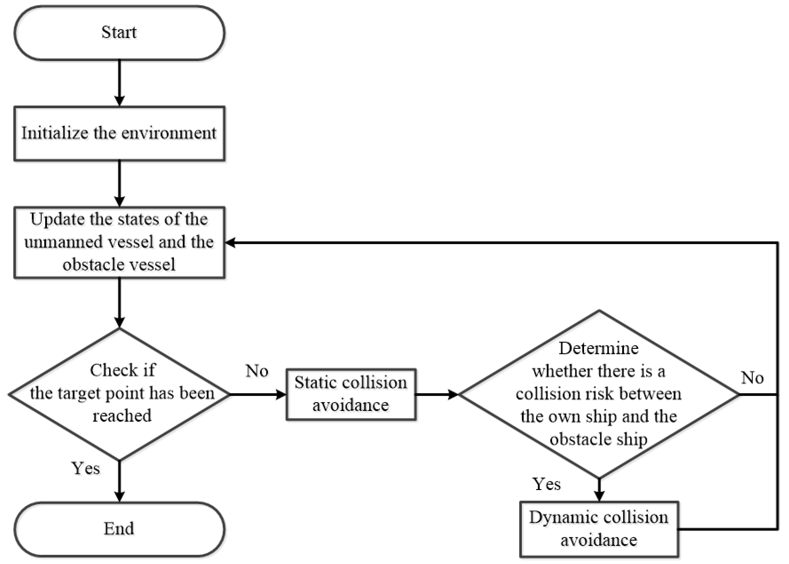
2. Methodology

2.1. Theoretical Background

This section first introduces the APF method, followed by collision risk theory, both of which are foundational to our research on safe navigation for USVs.

2.1.1. Artificial Potential Field (APF) Method

The APF [18] method is a popular path planning algorithm in robotics and autonomous navigation [19,20,21]. It uses virtual attractive and repulsive forces to help systems avoid obstacles and move toward a target. An attractive force field pulls the USV toward the target, while a repulsive force field keeps it clear of obstacles, ensuring safe navigation. Figure 1 shows the working principle of the APF, where orange circles represent obstacles, and the blue triangle marks the target point.

The attractive potential field function is

$$U_{att}={\displaystyle \frac{1}{2}}\eta d^2\left(x,x_{goal}\right),$$

(1)

where $x$ is the current position of the USV, $x_{goal}$ is the target position, $\eta$ is a positive scaling factor, and $d(x,x_{goal})$ is the distance and direction from the USV to the target.

The attractive force is

$$F_{att}=-\nabla U_{att}=-\eta d(x,x_{goal}).$$

(2)

The repulsive potential field function is

$$U_{rep}=\left\{\begin{array}{c}{\displaystyle \frac{1}{2}}k{({\displaystyle \frac{1}{d\left(x,x_{obs}\right)}}-{\displaystyle \frac{1}{d_0}})}^2,d\left(x,x_{obs}\right)\le d_0\\ 0,d\left(x,x_{obs}\right)>d_0\end{array}\right.,$$

(3)

where $x_{obs}$ is the position of the obstacle, $k$ is a positive scaling factor, and $d_0$ is the influence range of the obstacle.

The repulsive force is

$$F_{rep}=-\nabla U_{rep}=\left\{\begin{array}{c}k({\displaystyle \frac{1}{d\left(x,x_{obs}\right)}}-{\displaystyle \frac{1}{d_0}}){\displaystyle \frac{\nabla d(x,x_{obs})}{d^2(x,x_{obs})}},d\left(x,x_{obs}\right)\le d_0\\ 0,d\left(x,x_{obs}\right)>d_0\end{array}\right..$$

(4)

2.1.2. Ship Collision Risk

In the context of USV navigation, collision risk theory plays a crucial role in assessing the likelihood of collisions during encounters [22]. This theory evaluates the collision risk based on the relative positions, velocities, and environmental conditions of vessels, thus guiding decision-making in collision avoidance. Collision risk theory is integrated into the path planning process in this study to enhance the safety and reliability of USVs, ensuring effective responses to collision risks in various maritime scenarios. By accounting for dynamic vessel interactions, the theory helps determine the evasive maneuvers necessary to prevent potential collisions.

• The 1972 International Regulations for Preventing Collisions at Sea (COLREGs)

To apply collision risk theory in maritime navigation, it is important to follow international rules like the COLREGs. These rules, made for manned vessels, provide a safety framework for all vessels, including USVs. The 13th, 14th, and 15th Articles of the COLREGs outline guidelines for encounter situations that USVs may face while navigating [23].

• Overtaking: A vessel shall be deemed to be overtaking when coming up with another vessel from a direction more than 22.5 degrees abaft her beam. Any vessel overtaking any other shall must keep out of the way of the vessel being overtaken, as shown in Figure 2a;
• Head-on Situation: When two power-driven vessels are meeting on reciprocal or nearly reciprocal courses so as to involve risk of collision each shall alter her course to starboard so that each shall pass on the port side of the other, as shown in Figure 2b;
• Crossing Situation: When two power-driven vessels are crossing so as to involve risk of collision, the vessel which has the other on her own starboard side shall keep out of the way and shall, if the circumstances of the case admit, avoid crossing ahead of the other vessel, as shown in Figure 2c,d.

These provisions facilitate the secure navigation of unmanned vessels, aiding in effective collision avoidance and path planning within complex maritime environments [24,25,26,27].

2.

Distance of Closest Point of Approach (DCPA) and Time of Closest Point of Approach (TCPA)

In maritime collision avoidance, DCPA (distance to closest point of approach) and TCPA (time to closest point of approach) are widely utilized metrics for assessing potential collision risks [28,29].

DCPA represents the closest distance that two vessels will approach each other during an encounter, calculated based on their relative positions and velocities. Generally, a smaller DCPA leads to a higher likelihood of collision during the encounter. The formula for DCPA is

$$DCPA={\displaystyle \frac{\left|{\overrightarrow{r}}_B\left(t\right)-{\overrightarrow{r}}_A\left(t\right)\right|}{‖{\overrightarrow{v}}_A-{\overrightarrow{v}}_B‖}},$$

(5)

where, ${\overrightarrow{r}}_A\left(t\right)$ and ${\overrightarrow{r}}_B\left(t\right)$ are the positions of vessels A and B, and ${\overrightarrow{v}}_A$ and ${\overrightarrow{v}}_B$ are their velocity vectors.

TCPA represents the time it will take for the vessels to reach the closest point. This can be calculated by dividing DCPA by the relative velocity between the vessels:

$$TCPA={\displaystyle \frac{DCPA}{‖{\overrightarrow{v}}_A-{\overrightarrow{v}}_B‖}}.$$

(6)

3.

Space Collision Risk (SCR) and Time Collision Risk (TCR)

Collision risk incidence (CRI) is a measure of the likelihood of a collision between two vessels, ranging from 0 (no risk) to 1 (certain collision). The CRI can be divided into two components: space collision risk (SCR) and time collision risk (TCR) [30].

SCR measures the risk of a collision based on the closest point of approach (DCPA) between the vessels. The membership function for DCPA is defined as

$${\gamma }_{\mathrm{D}\mathrm{C}\mathrm{P}\mathrm{A}}=\left\{\begin{array}{c}1,\left|DCPA\right|<d_1\\ {\displaystyle \frac{1}{2}}-{\displaystyle \frac{1}{2}}sin\left[{\displaystyle \frac{\pi }{d_2-d_1}}\left(\left|DCPA\right|-{\displaystyle \frac{d_1+d_2}{2}}\right)\right]\\ 0,d_2<\left|DCPA\right|\end{array}\right.,d_1\le \left|DCPA\right|\le d_2,$$

(7)

where $d_1$ is the minimum safe distance, below which there is a high risk of collision, and $d_2$ represents the boundary where there is no collision risk. This function calculates the risk based on how close the vessels will get, with closer approaches indicating higher risks.

TCR assesses the urgency of avoiding a collision based on the time to the closest point of approach (TCPA). The membership function for TCPA is

$${\gamma }_{\mathrm{D}\mathrm{C}\mathrm{P}\mathrm{A}}=\left\{\begin{array}{c}1,TCPA\le t_1\\ {\left({\displaystyle \frac{t_2-TCPA}{t_2-t_1}}\right)}^2\\ 0,t_2<TCPA\end{array}\right.,t_1\le TCPA\le t_2,$$

(8)

where $t_1$ is the time it takes for the vessels to reach the closest point if they do not take evasive action. $t_2$ is the time threshold for when evasive action should be considered. The smaller the TCPA, the higher the urgency to avoid a collision.

The overall collision risk is a weighted combination of SCR and TCR:

$$\gamma =0.5{\gamma }_{\mathrm{D}\mathrm{C}\mathrm{P}\mathrm{A}}+0.5{\gamma }_{\mathrm{T}\mathrm{C}\mathrm{P}\mathrm{A}},$$

(9)

this combined risk helps assess the overall likelihood of a collision, guiding the necessary avoidance actions.

2.2. Path Planning Implementation

A path planning method for USVs is presented in this paper, combining the improved APF method with maritime regulations to address complex collision avoidance scenarios. The APF method helps guide the USV’s path by using attractive forces towards the target and repulsive forces to avoid obstacles. Additionally, the method adjusts the strength and direction of these forces based on the COLREGS. This ensures that the USV avoids collisions, while following the safety rules set by the regulations.

Figure 3 illustrates the main steps of the proposed method. In the environment generating process, the electronic nautical chart is turned into a raster map to create the navigation environment, and the boundary obstacles are identified. Then, the initial conditions for both the unmanned vessel and the obstacle vessel are set, including the unmanned vessel’s starting position, target, speed, and heading, as well as the obstacle vessel’s starting position and heading.

In the path planning process, the algorithm first checks if the USV has reached its target. If the USV has reached the target, the task is complete, and the path planning ends. If the target has not been reached, the algorithm proceeds to the next step, which is static collision avoidance. Then, based on the relative positions of the USV and the obstacle vessel, the algorithm evaluates if there is a risk of collision. If a collision risk is detected, the algorithm switches to dynamic collision avoidance mode. If no risk is found, the USV continues along its current path until it nears the target and completes the task.

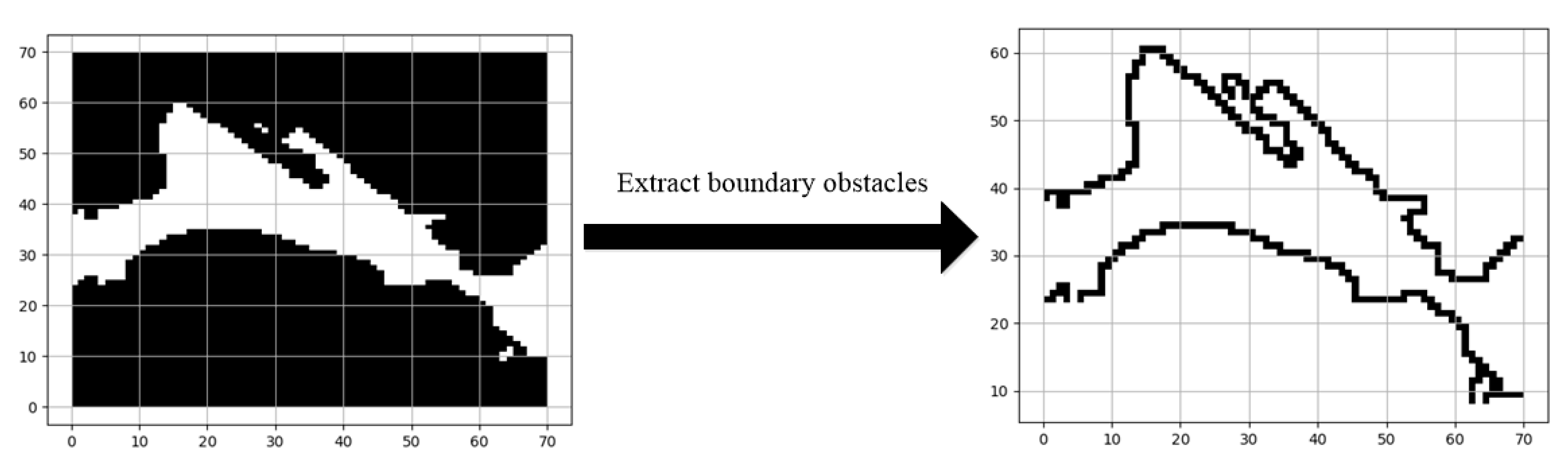
2.2.1. Discrete Boundary Potential Field Design

In traditional path planning algorithms, large obstacles are divided into smaller grid cells, and each of these grid cells generates a repulsive force to prevent the unmanned vessel from colliding with the obstacle. This method works well when obstacles are scattered and easy to avoid. However, in nautical chart scenarios, obstacles are often closely grouped together. If all obstacles create repulsive forces on the unmanned vessel, the algorithm might get stuck in local minima and become much slower. To solve this, using boundary potential fields is an important approach. Traditional algorithms are mainly designed for narrow channels, but in maritime environments with irregular boundaries, applying boundary potential fields is just as crucial to make path planning more efficient.

The method works as follows: First, the non-navigable areas of the nautical charts are converted into a raster format. Next, the boundary obstacles are identified, and a boundary potential field is created based on these obstacles.

Let $R(i,j)$ represent the raster grid, where

$$R(i,j)=\left\{\begin{array}{c}0,if\left(i,j\right)isanobstacle\\ 1,if(i,j)isnavigable\end{array}\right.,$$

(10)

where $(i,j)$ represents the position of the cell in the raster grid. A cell $R(i,j)$ is considered part of the boundary obstacle if it is an obstacle and has at least one adjacent cell that is navigable.

$$B\left(i,j\right)=1,ifR\left(i,j\right)=1and\exists R\left(i^{\prime },j^{\prime }\right)=0,$$

(11)

where $B\left(i,j\right)$ is the boundary indicator, and $\left(i^{\prime },j^{\prime }\right)\in \left\{\left(i+1,j\right),\left(i-1,j\right),\left(i,j-1\right),\left(i,j+1\right),\left(i+1,j-1\right),\left(i+1,j+1\right)\right\}$ are the adjacent cells.

To avoid collisions, the unmanned vessel only reacts to the repulsive forces from the boundary potential field. This approach is effective because, by focusing on the boundary obstacles, the vessel can still avoid collisions. Additionally, this method reduces the computational load, making the path planning process faster and more efficient.

By dividing the raster grid into sufficiently small cells, the boundary obstacles can be represented as a set of discrete points $P=\left\{\left(x_i,y_i\right)\right\}$. For each discrete point $P_i=(x_i,y_i)$, a repulsive potential field function is defined based on its distance $d$ from the main position $(x,y)$:

$$U\left(d\right)=\left\{\begin{array}{c}k·{\left({\displaystyle \frac{1}{d}}-{\displaystyle \frac{1}{d_{safe}}}\right)}^2,d<d_{safe}\\ 0,d\ge d_{safe}\end{array}\right.,$$

(12)

where $d=\sqrt{{\left(x-x_i\right)}^2+{\left(y-y_i\right)}^2}$, $d_{safe}$ is the effective range of the potential field, and $k$ is a parameter that adjusts the strength of the repulsive force.

The potential fields from all discrete points are superimposed to construct the overall boundary potential field:

$$U_{boundary}\left(x,y\right)={\sum }_i{U}_i\left(d_i\right).$$

(13)

At the same time, the contribution of each point to the potential field gradient (i.e., the repulsive force) is calculated as

$${\overrightarrow{F}}_{boundary}=\sum _i\nabla U_i\left(d_i\right)$$

(14)

where $\overrightarrow{r_i}=\left(x-x_i,y-y_i\right)$ is the vector from the main position to the point.

2.2.2. COLREGs-Based Collision Design

Figure 4 illustrates the dynamic collision avoidance phase of the algorithm. In this phase, the algorithm comprehensively considers the impact of moving obstacle vessels to ensure the safe navigation of the unmanned vessel in complex environments. First, the algorithm determines the encounter type based on the relative bearing and relative position between the two vessels, including head-on encounters, right crossings, left crossings, and overtaking situations. For a left crossing situation, the unmanned vessel will maintain its current course and end the collision avoidance task. For other situations, the algorithm calculates the safe passing distance (SCR) and time to collision (TCR), and further evaluates the potential collision risk.

If a collision risk is identified, the algorithm initiates an avoidance maneuver, in which the unmanned vessel turns a fixed number of degrees to the right to avoid the obstacle. Throughout the avoidance process, the algorithm continuously monitors the SCR and TCR and checks if there is still a collision risk. If the risk persists, the avoidance strategy will be iterated until the SCR satisfies the safe distance condition and the TCR meets the safe time condition, thereby ensuring the collision is successfully avoided. Finally, when no further collision risk exists, the vessel returns to its intended course, and the task is completed.

3. Simulation Results

3.1. Simulation Setup

The simulation was conducted in a rectangular area with boundaries defined by longitude 114.18° to 114.25° and latitude 22.26° to 22.33°. This area was discretized with a resolution of 0.001°, and a grid-based coordinate system was adopted. In this system, the coordinates are not based on latitude and longitude but are instead defined relative to the grid, starting from (0, 0) at the bottom-left corner. The boundaries of these obstacles were identified and marked, as shown in Figure 5. In this scenario, the black regions represent areas where potential fields are generated, while the white areas indicate navigable regions. The APF parameters used in the simulation were as follows: the attractive parameter $k_{att}$ was 15, the repulsive parameter $k_{rep}$ was 25, the effective range of the potential field $d_{safe}$ was 20, and the right turning angle ${\theta }_{right}$ was $1°$.

To evaluate the performance of the boundary potential field method in handling complex and irregular obstacle boundaries, comparative simulation experiments were designed and conducted. The traditional APF method combined with simulated annealing was used as the baseline, while the proposed boundary potential field method was tested as the experimental approach. The experiments were divided into two groups: in Experiment 1, 20 sets of coordinates were randomly selected as start and end points, and tests were performed using two different step sizes (0.01 and 0.05); in Experiment 2, 20 obstacles were randomly generated, and the 20 sets of start and end coordinates from Experiment 1 were tested again under the same two step size conditions. Key metrics, including arrival success rate, path length, and computation time, were recorded for each test.

To further showcase the algorithm’s ability to handle dynamic collision avoidance, simulations were performed following the COLREGS. Since no course change is needed in a left-crossing situation, this scenario was excluded. A simulation of two vessels encountering each other was conducted, with a route from the start point (20.87, 54.80) to the end point (30, 50) Three encounter scenarios were tested: head-on, overtaking, and right-crossing. These tests aimed to show how well the improved algorithm could adapt to real-world situations and effectively handle dynamic collision avoidance in various scenarios.

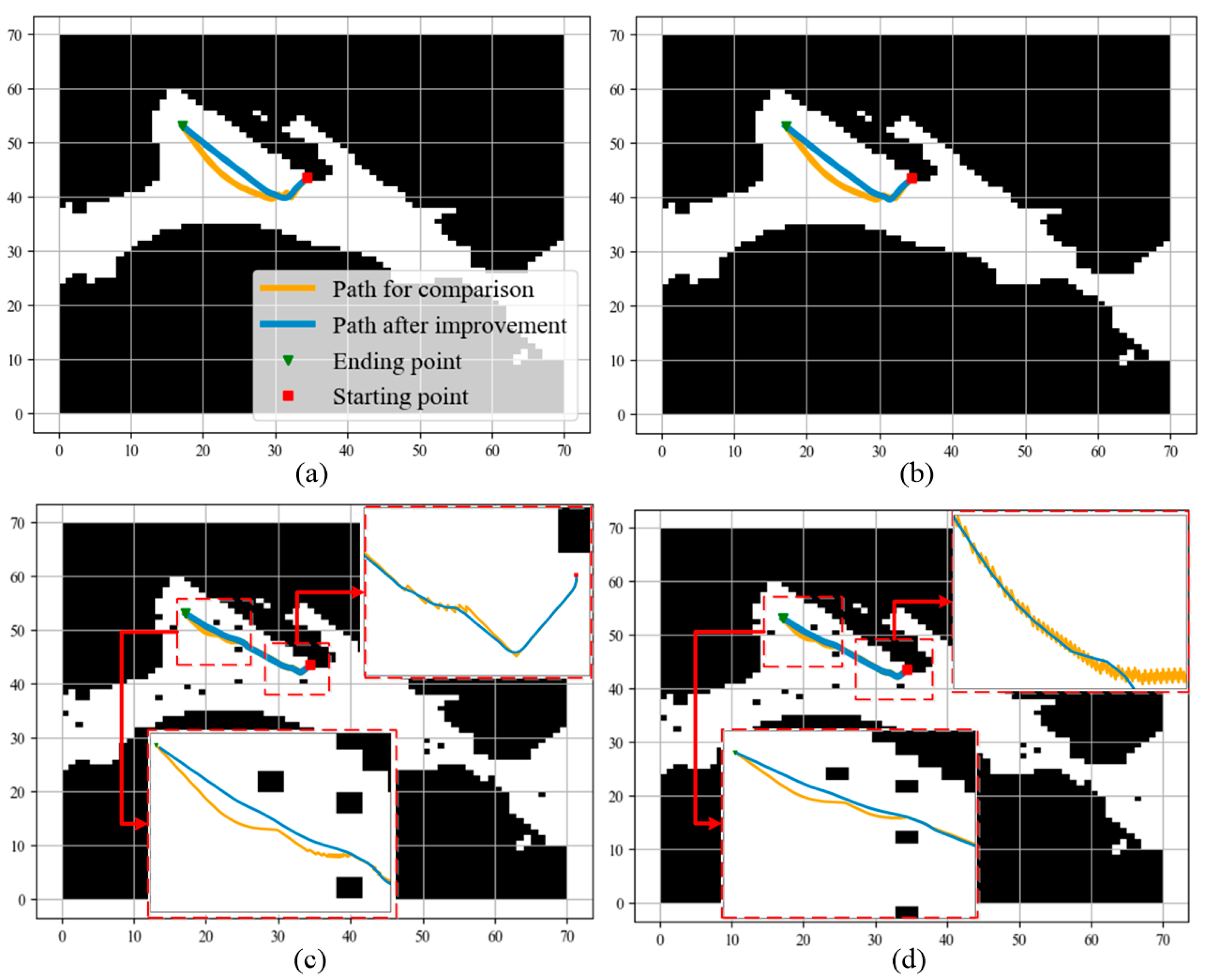
3.2. Static Environment Collision Avoidance

In Experiment 1, the arrival success rate was consistent across the different step sizes. The APF method combined with simulated annealing successfully reached the target 16 times, achieving an 80% success rate. In contrast, the improved boundary potential field method successfully reached the target in all 20 cases, achieving a 100% success rate. Similarly, in Experiment 2, the arrival success rate remained the same across the different step sizes. Consistently with the results of Experiment 1, the cases where the target was not reached in Experiment 1 also failed to reach the target in Experiment 2. However, the traditional method successfully reached the target only 12 times, resulting in a 60% success rate, while the improved method successfully reached the target in all 20 cases, maintaining a 100% success rate. This result indicates that the improved algorithm demonstrates higher stability and reliability when faced with more complex situations.

Figure 6 shows the results for cases where the target was successfully reached, comparing the performance of the traditional method and the improved algorithm in terms of path length and computation time under the different step sizes and obstacle conditions. Figure 6a,c compare the path length and computation time under the condition with no obstacles, while Figure 6b,d compare them under the condition with 20 random obstacles. Orange represents the traditional APF method combined with simulated annealing, and blue represents the improved boundary potential field algorithm. Dark colors indicate a step size of 0.01, while light colors represent a step size of 0.05.

In Figure 6a,b, although the yellow and blue lines are close to each other, the yellow line is generally above the blue line, indicating that the improved algorithm outperformed the traditional algorithm in terms of path length. Additionally, it can be observed that the dark and light lines nearly overlap, suggesting that the step size had little impact on the path length.

In terms of computation time, there was a significant difference between the two algorithms. In Figure 6c,d, it can be seen that the yellow line is consistently above the blue line, indicating that the improved algorithm outperformed the traditional algorithm in terms of computation time. Additionally, the dark lines are above the light lines, suggesting that smaller step sizes resulted in longer computation times. However, the dark blue line is only slightly higher than the light blue line, indicating that the step size had less impact on the improved algorithm. In contrast, the computation time of the traditional algorithm with a step size of 0.01 (dark yellow line) was much higher than that with a step size of 0.05 (light yellow line), which suggests that the traditional algorithm was more sensitive to the step size, leading to significantly longer computation times with smaller step sizes.

To visually demonstrate the improved performance of the proposed method, a path where both the improved algorithm and the traditional algorithm successfully reached the endpoint under four different conditions was selected, as shown in Figure 7. The starting point of the path was (34.38, 43.6), and the endpoint was (17.1, 53.2).

In Figure 7, the red square marks the starting point, the green triangle marks the endpoint, the yellow line represents the path of the APF method combined with simulated annealing, and the blue line represents the path of the APF method combined with the boundary potential field method. Additionally, key areas have been locally magnified for better visualization.

Figure 7a,b illustrate the path comparisons without random obstacles under step sizes of 0.05 and 0.01, respectively. Consistent with the experimental results for path length, the overall paths generated by the traditional algorithm and the improved algorithm were nearly identical under varying step size conditions. However, it is evident from the figures that the yellow path is longer and more convoluted than the blue path, demonstrating the superior performance of the improved algorithm.

Figure 7c,d depict the path comparisons in the presence of random obstacles under step sizes of 0.05 and 0.01, respectively. Similarly to the earlier results, the step size had minimal impact on the performance of both algorithms. However, when avoiding random obstacles, the path generated by the traditional algorithm (yellow line) was more winding and exhibited noticeable fluctuations, resulting in a longer path length. In contrast, the path generated by the improved algorithm (blue line) was shorter and smoother, underscoring its enhanced effectiveness in complex environments.

In summary, the improved algorithm not only achieved a significantly higher success rate than the traditional algorithm, but it also outperformed it in terms of both path length and computation time across the different test scenarios. By handling complex and irregular obstacles more effectively, the boundary potential field method reduced detours, shortened travel time, and improved the overall path planning efficiency. These advantages make it more suitable for practical applications.

3.3. Dynamic Environment Collision Avoidance

To further test the effectiveness of the improved algorithm in dynamic collision avoidance, a two-vessel encounter simulation was carried out. Unlike traditional dynamic collision avoidance approaches that typically ignore complex static obstacles, this scenario presented a significant challenge by incorporating both dynamic interactions and intricate static boundary obstacles, making it a more realistic and demanding test case.

Figure 8 shows the results of a head-on encounter scenario. In the figure, the yellow line represents the path of the obstacle vessel, the blue line shows the path generated by the proposed algorithm, and the black dots indicate the turning and course recovery points. The step size for the own ship was set to 0.015, while the obstacle vessel started at (44, 32.4) with a step size of 0.006, moving in a north-by-west 56-degree direction.

In this scenario, the unmanned vessel initially moved towards the center of the channel due to the influence of the boundary potential field (Figure 8a). When the own ship detected a collision risk with the obstacle vessel at (29.01, 42.57), it turned to the right (Figure 8b) to avoid the collision, which complied with COLREGS. As the vessel reached (33.42, 35.50), it detected that the collision risk had disappeared and returned to its original course (Figure 8c). Additionally, after recovering its course, the path near the destination exhibited a slight curvature due to the influence of the boundary potential field.

Figure 9 shows the results of a right-crossing encounter scenario. In this case, the own ship’s step size was set to 0.015, while the obstacle vessel started at (19, 37.2) and moved eastward with a step size of 0.01. As seen in Figure 9a, similarly to the head-on encounter scenario, the own ship initially headed toward the center of the channel under the influence of the boundary potential field. When it reached the position (22.76, 49.18), a collision risk was detected, prompting the vessel to turn right. Continuing its course to (27.13, 38.39), the collision risk with the obstacle vessel disappeared (Figure b), allowing the own ship to resume its original heading (Figure 9c).

Figure 10 shows the results of an overtaking scenario. The own ship had a step size of 0.01, while the obstacle vessel started at (26.6, 46.8) with a step size of 0.005, moving in the southeast direction at an angle of 50° east of south. In Figure 10a, similarly to the previous scenarios, the own ship first moved away from the boundary towards the center of the channel, and a collision risk was detected at (26.36, 45.08). In Figure 10b, the own ship turned right to overtake the obstacle vessel and successfully overtook it at (31.27, 38.98). In Figure 10c, the unmanned vessel recovered its course and continued towards the destination.

In summary, the proposed algorithm leveraged the advantages of the boundary potential field method to achieve dynamic collision avoidance in complex environments, while adhering to the COLREGS. The algorithm effectively addressed both static obstacles and dynamic collision risks, and optimized path planning by guiding the vessel with the boundary potential field, resulting in a smoother and more efficient avoidance process. Therefore, the algorithm demonstrated good stability and reliability in various complex scenarios, providing valuable insights for further research, with particularly significant potential for application in dynamic collision avoidance and complex navigation environments.

4. Discussion

Given the complexity of nautical chart scenarios, with many obstacles and irregular boundaries, and the challenges of applying COLREGs in such situations, an improved path planning method based on the boundary potential field technique was proposed in this paper. The method optimizes the navigation path and better incorporates the COLREGs, ensuring the safe sailing of unmanned vessels in complex environments.

Firstly, to reduce the computational burden caused by land obstacles in nautical charts, the boundary potential field method was introduced. This method simplifies obstacle handling and reduces both computation time and path length, particularly in areas with dense obstacles. Secondly, dynamic obstacle avoidance, considering the COLREGs, was incorporated into the path planning, building on the static collision avoidance using the boundary potential field method. This approach effectively implements dynamic obstacle avoidance in complex maritime environments, generating smooth paths. The simulation results showed that the boundary potential field method reduced the computation time and path length in static collision avoidance, while also performing well in dynamic obstacle avoidance when combined with maritime regulations.

Although progress has been made in this paper, there are still aspects that could be improved. For instance, the paper did not account for sudden course changes when encountering obstacle vessels that require emergency handling. Additionally, the effects of wind, waves, and currents could be incorporated into the model to better reflect real-world maritime conditions.

References

- Yunzhou Technology. Available online: www.yunzhou-tech.com/info/13900.html (accessed on 4 December 2024).
- Saildrone. Available online: www.saildrone.com/news/fleet-goes-on-mission-amid-already-busy-hurricane-season (accessed on 4 December 2024).
- Sedeño-Noda, A.; Colebrook, M. A biobjective Dijkstra algorithm. Eur. J. Oper. Res. 2019, 276, 106–118. [Google Scholar] [CrossRef]
- Dijkstra, E.W. A note on two problems in connexion with graphs. In Edsger Wybe Dijkstra: His Life, Work, and Legacy; Dijkstra, E.W., Ed.; Association for Computing Machinery: New York, NY, USA, 2022; pp. 287–290. [Google Scholar]
- Hart, P.E.; Nilsson, N.J.; Raphael, B. A formal basis for the heuristic determination of minimum cost paths. IEEE Trans. Syst. Sci. Cybern. 1968, 4, 100–107. [Google Scholar] [CrossRef]
- Sun, Y.; Fang, M.; Su, Y. AGV path planning based on improved Dijkstra algorithm. In Proceedings of the 3rd International Conference on Modeling, Simulation and Optimization Technologies and Applications (MSOTA), Beijing, China, 22–23 November 2020. [Google Scholar]
- Han, Z.; Wu, D.; Zhang, J.; Huang, T.; Han, Q.L.; Zhang, M. COLREGs-adaptive trajectory planning and decision-making in maritime autonomous surface ships. Ocean Eng. 2024, 312, 119308. [Google Scholar] [CrossRef]
- Xu, D.; Yang, J.; Zhou, X.; Xu, H. Hybrid path planning method for USV using bidirectional A and improved DWA considering the manoeuvrability and COLREGs. Ocean Eng. 2024, 298, 117210. [Google Scholar] [CrossRef]
- Karaman, S.; Frazzoli, E. Optimal kinodynamic motion planning using incremental sampling-based methods. In Proceedings of the 49th IEEE Conference on Decision and Control (CDC), Atlanta, GA, USA, 15–17 December 2010. [Google Scholar]
- Zhang, J.; Zhang, H.; Liu, J.; Wu, D.; Soares, C.G. A two-stage path planning algorithm based on rapid-exploring random tree for ships navigating in multi-obstacle water areas considering COLREGs. J. Mar. Sci. Eng. 2022, 10, 1441. [Google Scholar] [CrossRef]
- Chiang, H.T.L.; Tapia, L. COLREG-RRT: An RRT-based COLREGS-compliant motion planner for surface vehicle navigation. IEEE Robot. Autom. Lett. 2018, 3, 2024–2031. [Google Scholar] [CrossRef]
- Jadhav, A.K.; Pandi, A.R.; Somayajula, A. Collision avoidance for autonomous surface vessels using novel artificial potential fields. Ocean Eng. 2023, 288, 116011. [Google Scholar] [CrossRef]
- Liu, W.; Qiu, K.; Yang, X.; Wang, R.; Xiang, Z.; Wang, Y.; Xu, W. COLREGS-based collision avoidance algorithm for unmanned surface vehicles using modified artificial potential fields. Phys. Commun. 2023, 57, 101980. [Google Scholar] [CrossRef]
- Han, S.; Wang, L.; Wang, Y. A potential field-based trajectory planning and tracking approach for automatic berthing and COLREGs-compliant collision avoidance. Ocean Eng. 2022, 266, 112877. [Google Scholar] [CrossRef]
- Yuan, W.; Gao, P. Model predictive control-based collision avoidance for autonomous surface vehicles in congested inland waters. Math. Probl. Eng. 2022, 2022, 7584489. [Google Scholar] [CrossRef]
- Gan, L.; Yan, Z.; Zhang, L.; Liu, K.; Zheng, Y.; Zhou, C.; Shu, Y. Ship path planning based on safety potential field in inland rivers. Ocean Eng. 2022, 260, 111928. [Google Scholar] [CrossRef]
- Wang, Z.; Im, N. Enhanced artificial potential field for MASS’s path planning navigation in restricted waterways. Appl. Ocean Res. 2024, 149, 104052. [Google Scholar] [CrossRef]
- Khatib, O. Real-time obstacle avoidance for manipulators and mobile robots. Int. J. Robot. Res. 1986, 5, 90–98. [Google Scholar] [CrossRef]
- Lyu, H.; Yin, Y. COLREGS-constrained real-time path planning for autonomous ships using modified artificial potential fields. J. Navig. 2019, 72, 588–608. [Google Scholar] [CrossRef]
- Yao, Q.; Zheng, Z.; Qi, L.; Yuan, H.; Guo, X.; Zhao, M.; Liu, Z.; Yang, T. Path planning method with improved artificial potential field—A reinforcement learning perspective. IEEE Access 2020, 8, 135513–135523. [Google Scholar] [CrossRef]
- He, Z.; Chu, X.; Liu, C.; Wu, W. A novel model predictive artificial potential field based ship motion planning method considering COLREGs for complex encounter scenarios. ISA Trans. 2023, 134, 58–73. [Google Scholar] [CrossRef]
- Xu, Q.; Wang, N. A survey on ship collision risk evaluation. Promet-Traffic Transp. 2014, 26, 475–486. [Google Scholar] [CrossRef]
- International Maritime Organization (IMO). Convention on the International Regulations for Preventing Collisions at Sea, 1972 (COLREGs); IMO: London, UK, 1972. [Google Scholar]
- Naeem, W.; Henrique, S.C.; Hu, L. A reactive COLREGs-compliant navigation strategy for autonomous maritime navigation. IFAC-PapersOnLine 2016, 49, 207–213. [Google Scholar] [CrossRef]
- Lyu, H.; Yin, Y. Ship’s trajectory planning for collision avoidance at sea based on modified artificial potential field. In Proceedings of the 2017 2nd International Conference on Robotics and Automation Engineering (ICRAE), Shanghai, China, 29–31 December 2017. [Google Scholar]
- Huang, Y.; Zhao, S.; Zhao, S. Ship trajectory planning and optimization via ensemble hybrid A* and multi-target point artificial potential field model. J. Mar. Sci. Eng. 2024, 12, 1372. [Google Scholar] [CrossRef]
- Imazu, H.; Koyama, T. The determination of collision avoidance action. J. Jpn. Inst. Navig. 1984, 70, 31–37. [Google Scholar]
- Kang, L.; Lu, Z.; Meng, Q.; Gao, S.; Wang, F. Maritime simulator based determination of minimum DCPA and TCPA in head-on ship-to-ship collision avoidance in confined waters. Transp. A Transp. Sci. 2019, 15, 1124–1144. [Google Scholar] [CrossRef]
- Chen, G.; Huang, Z.; Wang, W.; Yang, S. A novel dynamically adjusted entropy algorithm for collision avoidance in autonomous ships based on deep reinforcement learning. J. Mar. Sci. Eng. 2024, 12, 1562. [Google Scholar] [CrossRef]
- Zheng, Z.Y.; Wu, Z.L. A new model of ship collision risk. J. Dalian Marit. Univ. 2002, 28, 1–5. (In Chinese) [Google Scholar]
Disclaimer/Publisher’s Note: The statements, opinions and data contained in all publications are solely those of the individual author(s) and contributor(s) and not of MDPI and/or the editor(s). MDPI and/or the editor(s) disclaim responsibility for any injury to people or property resulting from any ideas, methods, instructions or products referred to in the content. |
© 2025 by the authors. Licensee MDPI, Basel, Switzerland. This article is an open access article distributed under the terms and conditions of the Creative Commons Attribution (CC BY) license (https://creativecommons.org/licenses/by/4.0/).
Share and Cite
Li, Y.; Hou, P.; Cheng, C.; Wang, B. Research on Collision Avoidance Methods for Unmanned Surface Vehicles Based on Boundary Potential Field. J. Mar. Sci. Eng. 2025, 13, 88. https://doi.org/10.3390/jmse13010088
Li Y, Hou P, Cheng C, Wang B. Research on Collision Avoidance Methods for Unmanned Surface Vehicles Based on Boundary Potential Field. Journal of Marine Science and Engineering. 2025; 13(1):88. https://doi.org/10.3390/jmse13010088
Chicago/Turabian StyleLi, Yongzheng, Panpan Hou, Chen Cheng, and Biwei Wang. 2025. "Research on Collision Avoidance Methods for Unmanned Surface Vehicles Based on Boundary Potential Field" Journal of Marine Science and Engineering 13, no. 1: 88. https://doi.org/10.3390/jmse13010088
APA StyleLi, Y., Hou, P., Cheng, C., & Wang, B. (2025). Research on Collision Avoidance Methods for Unmanned Surface Vehicles Based on Boundary Potential Field. Journal of Marine Science and Engineering, 13(1), 88. https://doi.org/10.3390/jmse13010088