Investigation into the Prediction of Ship Heave Motion in Complex Sea Conditions Utilizing Hybrid Neural Networks

Abstract

While navigating at sea, ships are influenced by various factors, including wind, waves, and currents, which can result in heave motion that significantly impacts operations and potentially leads to accidents. Accurate forecasting of ship heaving is essential to guarantee the safety of maritime navigation. Consequently, this paper proposes a hybrid neural network method that combines Convolutional Neural Networks (CNNs), Bidirectional Long Short-Term Memory Networks (BiLSTMs), and an Attention Mechanism to predict the heaving motion of ships in moderate to complex sea conditions. The data feature extraction ability of CNNs, the temporal analysis capabilities of BiLSTMs, and the dynamic adjustment function of Attention on feature weights were comprehensively utilized to predict a ship’s heave motion. Simulations of a standard container ship’s motion time series under complex sea state conditions were carried out. The model training and validation results indicate that, under sea conditions 4, 5, and 6, the CNN-BiLSTM-Attention method demonstrated significant improvements in MAPE, APE, and RMSE when compared to the traditional LSTM, Attention, and LSTM-Attention methods. The CNN-BiLSTM-Attention method could enhance the accuracy of the prediction. Heave displacement, pitch displacement, pitch velocity, pitch acceleration, and incoming wave height were chosen as key input features. Sensitivity analysis was conducted to optimize the prediction performance of the CNN-BiLSTM-Attention hybrid neural network method, resulting in a significant improvement in MAPE and enhancing the accuracy of ship motion prediction. The research presented in this paper establishes a foundation for future studies on ship motion prediction.

1. Introduction

When ships navigate at sea, they are influenced by various factors such as wind, waves, and currents, leading to heave motions. The lack of control and prediction of these motions can result in serious impacts on operations and potentially cause accidents [1]. Forecasting methods rooted in hydrodynamic theory, such as the Kalman filter method, utilize principles of fluid mechanics pertaining to ships [2]. These methods simulate the flow field of a ship’s heaving motion in waves by numerically solving for the associated hydrodynamic coefficients and then predict the ship’s heaving motion based on these calculations [3,4]. On the one hand, this method is primarily utilized in the initial design of ships and for evaluating the ship’s heave motion response, but it falls short in providing short-term, real-time forecasting of the ship’s heave motion attitude during navigation. On the other hand, this method necessitates the acquisition of hydrodynamic coefficients, Lagrange boundary value conditions, power spectrum, and other relevant data, which entail a significant calculation load, leading to low calculation efficiency and potentially failing to meet practical engineering accuracy requirements for predictions.

Time series analysis serves as a crucial methodology for predicting ship motions. By utilizing time series data related to ship heave motion, a customized method for predicting such motion can be formulated, with the Auto-Regressive (AR) model serving as an example [5]. Furthermore, the Autoregressive Integrated Moving Average (ARIMA) method presents another viable alternative [6]. This methodology exclusively utilizes historical motion data of ships or waves for the purposes of modeling and predicting. Adopting this approach eliminates the need for complex physical modeling, thereby simplifying the prediction process while maintaining a high level of accuracy.

In recent years, advancements in artificial intelligence and nonlinear theory have led to an increasing use of neural network methods rooted in nonlinear theory for ship motion forecasting. Initially, the BP (Back Propagation) neural network was the pioneering artificial neural network in this domain [7,8,9]. Subsequently, the rapid evolution of GPU technology and machine learning algorithms has brought deep learning techniques to the forefront.

In this current research, scholars have employed Long Short-Term Memory (LSTM) neural network models to investigate the prediction of ship motion posture. To tackle the optimization issues associated with LSTM models, they have developed LSTM architectures with varying degrees of freedom (single, double, triple, and six degrees of freedom) and integrated coupled features to predict ship motions across low and moderate sea state conditions. Furthermore, numerous studies have utilized Bidirectional Long Short-Term Memory (BiLSTM) models to predict the pitch, heave, and roll motions of ships (Wang et al., 2012; Lawal et al.; Adytia et al., 2024; Benelmir et al., 2022; Jiang et al., 2024; Wei et al., 2022; Zhang et al., 2023; Li et al., 2022) [10,11,12,13,14,15,16,17]. In general, previous studies have shown that standalone neural network methods perform well in predicting ship motions, but they mainly focus on low and moderate sea states; standalone neural network models still face challenges in complex sea conditions.

Conventional probabilistic approaches demonstrate greater sensitivity to linear datasets, whereas neural network techniques show superior accuracy in predicting intricate nonlinear data. To effectively describe the heaving motion of ships and greatly enhance prediction precision, hybrid forecasting techniques utilizing neural networks have been extensively employed to predict ship heaving behavior. These methods integrate neural networks with wavelet decomposition, hyperparameter optimization, and feature extraction techniques [18,19,20,21,22,23,24]. Currently, there is limited research on forecasting ship motion using deep neural network technology, with most studies relying on somewhat idealized ship motion forecasting data. The effectiveness and robustness of ship motion forecasting techniques based on deep neural networks still necessitate further validation [25].

Inspired by the latest studies, this study focuses on the prediction of ship heave motions in complex sea conditions, comprehensively investigating the effects of the feature variables and designing the specific learning algorithm. To address the aforementioned issue, this paper introduces a CNN-BiLSTM-Attention hybrid neural network method for short-term forecasting of ship heaving motion in waves. Firstly, a CNN is used to extract features of ship motion and environmental conditions. Subsequently, the extracted feature sequences are fed into the bidirectional LSTM layers, which analyze the inherent relationships between the current data and both past and future data, considering both forward and backward directions. An Attention mechanism is integrated to assign different weights to various features, thereby enhancing the importance of significant features. Ultimately, the SHAP sensitivity coefficient analysis method is utilized to filter ship motion and environmental parameters, with the aim of eliminating feature redundancy and enhancing the accuracy of the CNN-BiLSTM-Attention neural network method.

The main content of this paper is organized into six sections. Section 2 introduces the internal structure of the CNN-BiLSTM-Attention model. Section 3 provides a detailed description of the data sources utilized in this study. Section 4 presents several common neural network forecasting models and compares them with the CNN-BiLSTM-Attention model to validate its effectiveness and investigate the impact of input sequence length on forecasting accuracy. Section 5 employs SHAP sensitivity analysis to select ship motion and environmental features, thereby enhancing the accuracy of the CNN-BiLSTM-Attention model. Section 6 further validates the aforementioned procedures using the KCS ship model under level four sea conditions, traveling at a speed of 20 knots, and a heading of 150°. Finally, Section 7 summarizes the findings of this paper.

2. Neural Networks

In this study, we propose a CNN-BiLSTM-Attention hybrid neural network model to predict the heave motion of ships under moderate to complex sea conditions. The model begins by receiving pre-processed ship motion and environmental data through the input layer. Subsequently, feature extraction is performed via the CNN layer. These extracted features are then fed into the BiLSTM layer for temporal analysis. Finally, an Attention mechanism is applied to weigh the key features, thereby enhancing the model’s predictive accuracy. This chapter will provide a detailed description of the model’s internal structure and working principles, along with its integration of CNN, BiLSTM, and Attention mechanisms to achieve the forecasting of ship heave motion.

2.1. Convolutional Neural Networks

A Convolutional Neural Network (CNN) is a feedforward neural network characterized by convolutional computations and a deep learning architecture. The network structure within a CNN consists of an input layer, hidden layers, and an output layer. The hidden layers include convolutional layers, pooling layers, and fully connected layers, which are interconnected through activation functions and undergo nonlinear transformations. Each convolutional and pooling layer performs feature extraction and down-sampling operations on the input data, with the results automatically passed to the subsequent layer. The fully connected layer maps the features extracted by the preceding layers to the final output [26]. Due to their multi-layer neural network structure, CNNs are capable of learning features at various levels of abstraction.

Convolutional Neural Networks (CNNs) employ convolutional operations during the computation process, thereby enhancing the efficiency of matrix operations. The convolutional and pooling layers are responsible for feature extraction and dimensionality reduction in features. Figure 1 illustrates a typical structure of a Convolutional Neural Network.

2.2. Bidirectional Long Short-Term Memory Network

As shown in Figure 2, the Bidirectional Long Short-Term Memory (BiLSTM) neural network signifies refined enhancement compared to the conventional unidirectional Long Short-Term Memory (LSTM) network. A BiLSTM comprises two standard LSTMs—a forward LSTM layer and a backward LSTM layer—both of which contribute to the generation of the final output. The unidirectional LSTM is limited to extracting feature information from time series data in a forward direction, from past to future, and lacks the ability to capture information from future to past. This limitation may result in decreased learning efficiency in ship ultra-short-term motion prediction methods and adversely affect the method’s predictive accuracy [27,28]. By contrast, the BiLSTM captures time series data information in both directions, enabling it to utilize ship motion data from past moments and to learn features from future moments. This continuous improvement in the learning capability of the neural network prediction method, coupled with the enhanced utilization rate of time series data, subsequently results in improved predictive accuracy.

2.3. Attention Mechanism

The Attention mechanism in deep learning emulates the human process of selective focus. When humans observe their surroundings, they quickly scan the entire scene to identify objects that require focused attention. Subsequently, they focus their attention on these focal points, considering them key elements while automatically discarding irrelevant details. Similarly, the Attention mechanism is fundamentally a process of resource reallocation, where the internal neural network assigns different weights to input data based on the importance of the information. This enables the mechanism to focus its attention on the critical parts. Consequently, the Attention mechanism can learn autonomously and selectively prioritize key information within the input. It addresses the issue of information loss in recurrent neural networks when handling long-range sequences, enhances computational efficiency, and improves the method’s performance and generalization capabilities [29]. The basic framework of the Attention mechanism is depicted in Figure 3.

The vectors $Q$ (query matrix), $K$ (key matrix), and $V$ (value matrix) are derived from the input features. Here, $Q$ represents the query matrix, $K$ represents the key matrix, and $V$ represents the value matrix. These vectors represent the input features, and the feature vectors used to compute the attention weights are also derived from the input features. The Attention mechanism multiplies the vectors by their respective weights, based on the level of attention assigned to each. The self-Attention mechanism can be formulated as follows:

$$\left\{\begin{array}{c}Q=X{W}^Q\\ K=X{W}^K\\ V=X{W}^{\nu }\end{array}\right.$$

(1)

$$output=softmax({\displaystyle \frac{Q{K}^T}{\sqrt{d}}})V$$

(2)

The vectors $Q$, $K$, and $V$ are obtained from the input matrix $X$ through linear transformations. The Attention mechanism does not directly use $X$, but instead the input matrix $X$ is multiplied by $W^Q$, $W^K$, and $W^{\nu }$ to generate $Q$, $K$, and $V$, respectively, with each undergoing a linear transformation. Utilizing these three trainable parameter matrices enhances the fitting capability of the neural network method. Equation (2) represents the core formula of the Attention mechanism.

$d$ denotes the dimensionality of Q and K, and the Softmax function, also known as the normalized exponential function, is an activation function that compresses any N-dimensional real vector to a vector in the range (0, 1) with all elements summing to 1. Dividing by $\sqrt{d}$ helps to scale the data, preventing the vanishing gradient problem.

2.4. CNN-BiLSTM-Attention Neural Network Method

To enhance the precision of predicting the motion status of ships, this study introduces a hybrid neural network approach that integrates Convolutional Neural Networks (CNNs), Bidirectional Long Short-Term Memory (BiLSTM), and Attention mechanisms for the short-term predicting of ship heaving motion in wave conditions, as depicted in Figure 4. The internal hyperparameter settings of the network are shown in

Table 1. Structures of the proposed method.

Block	Layer	Number/Size/Stride of Kernels or Number of Neurons
Feature extraction block	Conv1	[32, 64, 128, 256]/64/1
	Max-pooling	[32, 64, 128, 256]/2/1
	Flatten	-
Sequence learning block	BiLSTM1	[32, 64, 128, 256]
Attention block	Attention	[32, 64, 128, 256]
Prediction block	FC1	[32, 64, 128, 256]
	FC2	20

.

3. Case Study

For complex sea conditions with a large amplitude of ship motions, available datasets are scarce due to high cost and navigational safety risks. CFD-based methods provide a way to obtain relatively realistic numerical results [30,31,32,33]. Datasets play a key role in model training and evaluation. However, available datasets for complex sea states are scarce due to the high cost and navigational safety risks. In this study, a technique based on CFD is applied to obtain fidelity data on ship motion in complex sea conditions.

The CNN-BiLSTM-Attention neural network, proposed for characterizing the heave motion of ships, was demonstrated using a hydrodynamic software simulation for a KCS hull shape. The basic parameters of the KCS ship are shown in

Table 2. Dimension of KCS.

Dimensions	Units	Value
Length between the perpendiculars	m	230.00
Beam at waterline	m	32.20
Beam at waterline	m	32.20
Depth	m	19.00
Draft	m	10.80
Displacement	m3	52,030.00
Longitudinal center of gravity from the aft	m	111.60
Design speed	kn	20.00

. The core of the CFD calculation scheme lies in solving the interaction problem between waves and the hull. Firstly, the Pierson-Moskowitz (P-M) two-parameter wave spectrum method is utilized to simulate the generation and evolution of ocean waves. The specific formula is presented in Equation (3). The initial boundary value problem is then solved using the potential flow boundary element method, followed by the calculation of the hull pressure distribution, including the second-order term, using Bernoulli’s equation, to obtain the three-dimensional perturbed velocity potential.

When a ship navigates in wind and waves, it is influenced by the wind, waves, and currents, resulting in a coupled motion characterized by six degrees of freedom. In addition to the effects of sea wind and waves, nonlinear and complex interdependencies exist among various influencing factors during the ship’s navigation. To improve the forecasting accuracy of the ship’s heaving motion, it is crucial to consider other time-series data that are highly correlated with the motion being predicted and to refine the existing methods of ship motion prediction. By integrating the inherent connections among data, we can attain more precise forecasting outcomes based on this framework. It is important to highlight that the subsequent discourse is founded on the equations that dictate the ship’s swaying motion [34].

$$\left(I_{\mathrm{xx}}+\Delta I_{\mathrm{xx}}\right)\ddot{\varphi }+2N_{xx}\dot{\varphi }+D_{xx}\varphi =F_{roll}$$

(3)

$$\left(I_{\mathrm{yy}}+\Delta I_{yy}\right)\ddot{\varphi }+2N_{yy}\dot{\varphi }+D_{yy}\varphi =F_{pitch}$$

(4)

$$Z=Z_{m}sin({\omega }_{h}t+a)$$

(5)

In the above equations, where $I_{\mathrm{xx}}$ and $I_{\mathrm{yy}}$ are the moments of inertia of the ship around the x-axis and y-axis, $\Delta I_{\mathrm{xx}}$ and $\Delta I_{yy}$ are the changes in the moments of inertia caused by the added masses; $N_{xx}$ and $N_{yy}$ are the damping coefficients for roll and pitch; and $D_{xx}$ and $D_{yy}$ are the restoring moments. $Z$ is the vertical displacement of the hull, $Z_m$ is the amplitude, representing the maximum displacement of the ship’s heave motion, and $a$ is the phase angle, indicating the initial phase of the ship’s motion relative to a certain reference point.

It is widely recognized that there is not only an interdependent relationship among roll, pitch, and heave motions but also a significant correlation with the forces exerted on the ship and its present location.

Variations in scattering intensity and frequency can lead to a significant reduction in the average values of heave motion and its velocity amplitude, consequently diminishing the intensity of the ship’s heaving motion. When evaluating the influence of waves on vessel dynamics, the height of incoming waves (which correlates with scattering intensity) may have a more significant impact on heave motion compared to wave velocity (which is related to scattering frequency) [35]. As a result, this study selects incoming wave height as an environmental variable to analyze its influence on short-term ship motion forecasting.

Based on the analysis above, this paper ultimately employs the CFD to calculate the ship motion data for a container ship traveling at a speed of 20 knots in head seas, specifically under sea states four, five, and six, at a heading of 180°. The selected ship motion data, which serves as model input features, includes the roll velocity, heave velocity, pitch velocity, roll displacement, heave displacement, pitch displacement, roll acceleration, heave acceleration, pitch acceleration, and incoming wave.

In the analysis of ship heaving motion and their influence on wave patterns, it is essential to identify the key parameters of significant incoming wave height (Hs) and characteristic period (Tp) across various maritime conditions. The significant incoming wave height represents the average height of the highest one-third of the waves, whereas the characteristic period signifies the average time interval between consecutive waves. These two parameters serve as key indicators for describing sea states. The process of selecting the significant incoming wave height (Hs) and characteristic period (Tp) is intricate and requires the evaluation of various factors, such as wave properties, ship specifications, hydrodynamic coefficients, frequency distribution of encounters, wave orientation, ship handling capabilities, and environmental conditions [36].

The dataset utilized in the experiment was sourced through simulation, utilizing CFD software [37] to compute the motion data of a container ship traveling at 20 knots in head seas under sea states four, five, and six. This dataset primarily encompassed the ship’s roll angle, heave displacement, pitch angle, roll angular velocity and acceleration, heave velocity and acceleration, pitch angular velocity and acceleration, and incoming wave. Figure 5a,b depict partial raw data regarding the ship’s heave motion and an instance dataset.

4. Date Validation

4.1. Error Assessment Criteria

To assess the performance of the selected method, this paper employs the Mean Absolute Percentage Error (MAPE), Absolute Percentage Error (APE), and Root Mean Square Error (RMSE) as evaluation metrics for the forecasting results. The specific calculation formulas are as follows:

$$\mathrm{MAPE}={\displaystyle \frac{1}{n}}{\displaystyle \sum _{i=1}^n\left|\frac{\widehat{x}(i)-x(i)}{x(i)}\right|}\times 100\%$$

(6)

$$APE={\displaystyle \frac{{\max }_{1\le i\le n}\left(\left|\widehat{x_i}-x_i\right|\right)}{x_i}}$$

(7)

$$\mathrm{RMSE}=\sqrt{{\displaystyle \frac{{\displaystyle \sum _{j=1}^n}{\left(x_j-{\widehat{x}}_j\right)}^2}{n}}}$$

(8)

The Root Mean Square Error (RMSE) quantifies the average magnitude of discrepancies between observed and predicted values, whereas the Mean Absolute Percentage Error (MAPE) reflects the average percentage divergence of the predicted values from the actual values. Considering the relatively low magnitude of the values within the dataset, employing RMSE as a loss function could yield a loss value that appears numerically insignificant, despite potentially inadequate forecasting performance. Therefore, in our simulation experiments, we adopt the key metric MAPE as the primary loss function. It is important to highlight that RMSE serves as a significant error metric in the experiment, as it accurately represents the predictive precision of the neural network approach concerning absolute discrepancies.

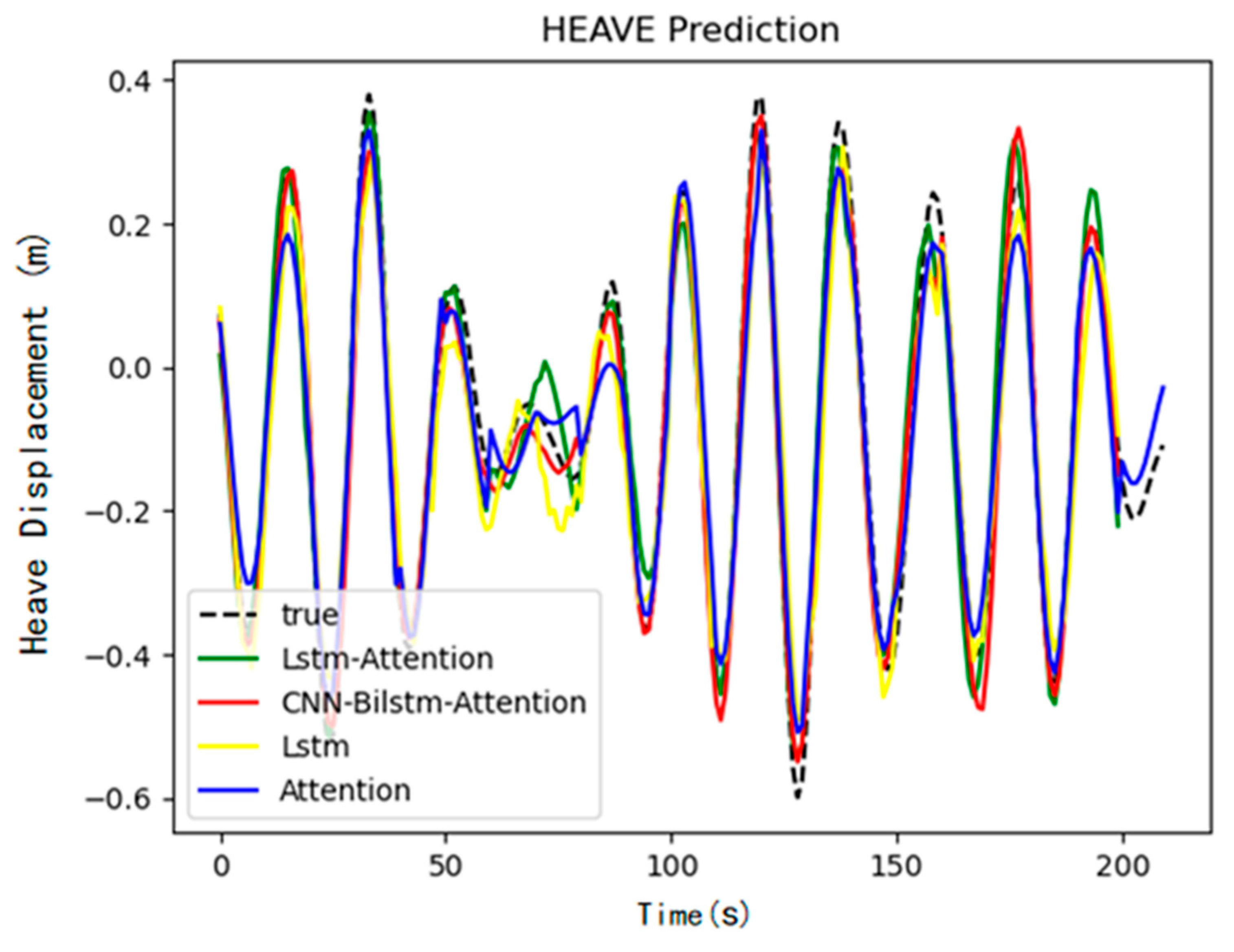
4.2. Comparison of Forecasting Accuracy of Different Methods

In this research, we compared the forecasting accuracy of various models for predicting the heave motion of ships under different sea conditions. The models under consideration included Long Short-Term Memory (LSTM), Attention, LSTM-Attention, and CNN-BiLSTM-Attention. The input data for these models comprised roll, pitch, heave, roll angular velocity, pitch angular velocity, heave velocity, roll angular acceleration, pitch angular acceleration, heave acceleration, and incoming wave measured 5 m ahead of the bow. The internal hyperparameter settings of the network are shown in

Table 3. Modeling parameters.

Method	Epoch	Search Scope	Learning Rate
LSTM	300	[32, 64, 128, 256]	0.001–0.0001
Attention	300	[32, 64, 128, 256]	0.001–0.0001
LSTM-Attention	300	[32, 64, 128, 256]	0.001–0.0001
CNN-BiLSTM-Attention	300	[32, 64, 128, 256]	0.001–0.0001

. The training period (Epoch) for all models was uniformly set at 300, and early stopping was utilized to enhance the training procedure with various optimizers. The validation loss (val_loss) on the validation dataset acted as the benchmark for implementing early stopping. If the validation loss did not show improvement of at least a defined threshold (min_delta = 1 × 10⁻²) over the course of 50 epochs, the model training was considered finished, and the training process was halted. The prediction errors for the various methods under sea state four, five, and six conditions are detailed in the Figure 6, Figure 7 and Figure 8 and

Table 4. Forecasting errors of different methods under sea-state-four conditions.

Algorithm Method	MAPE (%)	APE (%)	RMSE
LSTM	39.8529	34.7442	0.0047
Attention	45.0247	51.0200	0.0087
LSTM-Attention	34.0827	30.6340	0.0044
CNN-BiLSTM-Attention	20.6654	2.3391	0.0049

,

Table 5. Forecasting errors of different methods under sea-state-five conditions.

Algorithm Method	MAPE (%)	APE (%)	RMSE (%)
LSTM	52.1384	37.3193	0.0511
Attention	61.8964	57.691	0.0652
LSTM-Attention	39.8529	34.7442	0.0466
CNN-BiLSTM-Attention	13.7541	16.1682	0.0296

and

Table 6. Forecasting errors of different methods under sea-state-six conditions.

Algorithm Method	MAPE (%)	APE (%)	RMSE
LSTM	85.8167	63.4507	0.1371
Attention	87.7659	63.4866	0.1382
LSTM-Attention	59.5770	23.4311	0.0922
CNN-BiLSTM-Attention	55.1988	8.5259	0.0741

.

Taking sea state four as an example, the Mean Absolute Percentage Error (MAPE) for the LSTM, Attention, LSTM-Attention, and CNN-BiLSTM-Attention methods were 39.8529%, 45.0247%, 34.0827%, and 20.6654%, respectively. The Absolute Percentage Error (APE) for these methods was 34.7442%, 51.0200%, 30.6340%, and 23.391%, respectively; the Root Mean Square Error (RMSE) was 0.0047, 0.0087, 0.0044, and 0.0049, respectively (note: RMSE values are typically not expressed in percentage form). By synthesizing the statistical errors, it can be observed that the CNN-BiLSTM-Attention method exhibits the smallest forecasting error across different datasets. As the lead steps increase, the forecasting errors of the LSTM, Attention, and LSTM-Attention networks tend to be larger than those of the CNN-BiLSTM-Attention network.

4.3. The Impact of Input Sequence Length on Forecasting Accuracy

The length of the input sequence influences the precision and effectiveness of machine learning techniques. In this section, we utilize the heaving motion of a ship in oblique waves as a test case. By comparing the forecasting accuracy associated with various lengths of input data and considering the time required for method training and forecasting, we comprehensively determine the optimal input data length suitable for this method. The input sequence length varies from 20 to 100, which corresponds to a duration of 10 to 50 s, assuming each unit length equates to 0.5 s. The Mean Absolute Error (MAE) serves as the loss function. The CNN-BiLSTM-Attention hybrid neural network method employs stochastic gradient descent with a learning rate of 0.001 and utilizes the Dropout method to mitigate method overfitting [38]. A batch training approach is utilized, featuring a batch size of 128 data samples for each iteration. The predicted results are shown in

Table 7. Forecasting results of the CNN-BiLSTM-Attention method under sea state four conditions.

Input Sequence Length	MAPE (%)	APE (%)	RMSE
20	40.0913	17.8982	0.0088
30	28.4440	7.4996	0.0065
40	27.7298	11.7755	0.0073
50	25.9142	9.3645	0.0065
60	21.9325	2.8663	0.0050
70	23.0533	5.188	0.0049
80	20.6654	2.3391	0.0049
90	40.0913	17.8982	0.0088
100	28.444	7.4996	0.0065

,

Table 8. Forecasting results of the CNN-BiLSTM-Attention method under sea state five conditions.

Input Sequence Length	MAPE (%)	APE (%)	RMSE
20	20.922	23.9372	0.0509
30	16.1432	14.7023	0.0450
40	27.9656	16.9696	0.0433
50	16.2810	2.9479	0.0384
60	17.1256	14.2950	0.0424
70	18.4146	13.6242	0.0416
80	13.4406	12.1682	0.0354
90	14.4060	14.9068	0.0422
100	15.9607	15.6451	0.0406

and

Table 9. Forecasting results of the CNN-BiLSTM-Attention method under sea state six conditions.

Input Sequence Length	MAPE (%)	APE (%)	RMSE
20	63.3917	5.7230	0.0848
30	49.9763	5.1494	0.0816
40	72.2531	9.3186	0.0907
50	54.0273	8.7084	0.0761
60	50.0174	8.0507	0.0761
70	58.2433	6.3570	0.0844
80	50.1988	5.5259	0.0741
90	53.9695	5.9610	0.0816
100	68.8507	7.1328	0.0667

and Figure 9, Figure 10 and Figure 11.

An input sequence that is excessively brief may impede the method’s capacity to gather adequate historical data, thus undermining its predictive efficacy; conversely, an excessively lengthy input sequence may include superfluous information, intensifying the computational load on the method and potentially heightening the likelihood of overfitting. Considering the periodic nature of the heaving motion and the computational efficiency of the hybrid neural network approach, an input sequence length of 80 has been determined. This selection not only allows the method to utilize essential historical data for precise predictions but also reduces the negative impacts linked to overly lengthy sequences.

This chapter validates the effectiveness of the proposed CNN-BiLSTM-Attention method for ultra-short-term forecasting of ship heaving motion by comparing it with LSTM, Attention, and LSTM-Attention neural network methods. The Mean Absolute Percentage Error (MAPE), Absolute Percentage Error (APE), and Root Mean Square Error (RMSE) are employed as evaluation metrics. The results reveal that under sea states four, five, and six, the CNN-BiLSTM-Attention method achieved reductions in MAPE by 54.10%, 78.23%, and 37.11%, respectively, and reductions in APE by 95.41%, 78.23%, and 86.57%, respectively, thereby demonstrating higher predictive accuracy and stability compared to the other methods. Additionally, the influence of input sequence length on the forecasting accuracy of the method was examined, leading to the identification of an optimal input sequence length. This further reinforces the exceptional efficacy of the CNN-BiLSTM-Attention approach in predicting ship motion.

5. Sensitivity Analysis Study

Sensitivity analysis is a technique within uncertainty analysis that quantitatively evaluates the extent to which variations in pertinent factors affect one or a series of key indicators. Essentially, it involves systematically manipulating each input variable according to a predefined pattern and then scrutinizing the resultant impact on the output variable, often expressed through sensitivity indices.

5.1. Basic Principles

Since this paper is focused on ultra-short-term ship motion forecasting, a type of time series prediction, the most common sensitivity analysis methods generally employ random sampling in data processing. However, this approach fails to capture temporal sequence characteristics. Acknowledging these limitations, this paper employs the versatile and interpretable machine learning method, SHAP (Shapley Additive explanations), for sensitivity analysis. SHAP is a game-theory-based method utilized for interpreting machine learning methods. It approximates complex machine learning methods with a collection of linear models and computes the SHAP values within these linear approximations to analyze the contribution of each feature to the prediction results. This approach provides a deeper understanding of the decision-making process of machine learning models and facilitates the selection of appropriate input features. The formula for calculating SHAP values is provided as follows:

$${\varphi }_i=\sum _{S\subseteq N(i)}{\displaystyle \frac{\left|S\right|!\left(M-\left|S\right|!-1\right)}{M!}}[f_x\left(S\cup \left\{i\right\}\right)-f_x\left(S\right)]$$

(9)

In the formula, ${\varphi }_0$ represents the contribution of the i-th feature; $N$ represents the set of all features; $S$ represents a subset of the prediction features given; $f_x\left(S\cup \left\{i\right\}\right)$ and $f_x\left(S\right)$, respectively, represent the method results including or excluding the i-th feature. SHAP approximates complex methods by constructing multiple linear methods and defines the output of the method $g\left(z^{\prime }\right)$, with M features as a linear sum of the contributions of the input variables.

$$g\left(z^{\prime }\right)={\varphi }_0+\sum _{i=1}^M{\varphi }_i{z}_i^{\prime }$$

(10)

In the formula, ${\varphi }_0$ represents the prediction result without any feature values; ${\varphi }_i$ is the Shapley value of the i-th feature; and $z_i^{\prime }$ indicates 1 when the i-th feature is selected and 0 otherwise.

5.2. Input Parameter Study

To enhance the forecasting accuracy of ship heaving motion, it is not only necessary to explore the impact of input sequence length but also to consider other time-series data that are strongly correlated with the ship’s predicted motion. By refining the current methods of ship motion forecasting and incorporating the intrinsic connections between the data, more accurate forecasting results can be achieved on this basis.

Consequently, the parameters selected for sensitivity analysis include roll, pitch, heave, roll angular velocity, pitch angular velocity, heave velocity, roll angular acceleration, pitch angular acceleration, heave acceleration, and incoming wave height at the 5 m position at the bow. Utilizing the inputs from the preceding section, a sensitivity analysis was conducted to forecast the heaving motion of the container ship under various sea conditions, particularly in the context of 180° head-on waves and a vessel speed of 20 knots. The objective of this analysis is to identify the optimal parameter set for diverse operational scenarios. The results of the sensitivity analysis are shown in

Table 10. Sensitivity analysis statistics table for heave motion forecasting results under sea state four conditions.

Input Parameters	Shap	Percentage
Heave Dis	0.0066141	25.16%
Roll Dis	0.00007005	0.27%
Pitch Dis	0.00600698	22.85%
Heave Vel	0.0024635	9.37%
Roll Vel	0.0000934	0.36%
Pitch Vel	0.00350261	13.32%
Heave Acc	0.00157618	6.00%
Roll Acc	0.00003503	0.13%
Pitch Acc	0.00398714	15.17%
Incoming wave	0.00193811	7.37%

,

Table 11. Statistical table of sensitivity analysis for heave motion prediction results under sea state five conditions.

Input Parameters	Shap	Percentage
Heave Dis	0.00378004	13.05%
Roll Dis	0.00005906	0.20%
Pitch Dis	0.00669777	23.12%
Heave Vel	0.00235071	8.12%
Roll Vel	0.00005316	0.18%
Pitch Vel	0.00199267	5.78%
Heave Acc	0.00376823	13.01%
Roll Acc	0.00004725	0.16%
Pitch Acc	0.00399267	13.78%
Incoming wave	0.00422302	14.58%

and

Table 12. Sensitivity analysis statistics table for heave motion forecasting results under sea state six conditions.

Input Parameters	Shap	Percentage
Heave Dis	0.00294686	11.58%
Roll Dis	0.00004911	0.19%
Pitch Dis	0.00475317	18.68%
Heave Vel	0.0017954	7.06%
Roll Vel	0.00004366	0.17%
Pitch Vel	0.00247209	9.72%
Heave Acc	0.00266309	10.47%
Roll Acc	0.00003274	0.13%
Pitch Acc	0.00449669	17.67%
Incoming wave	0.00618840	24.32%

.

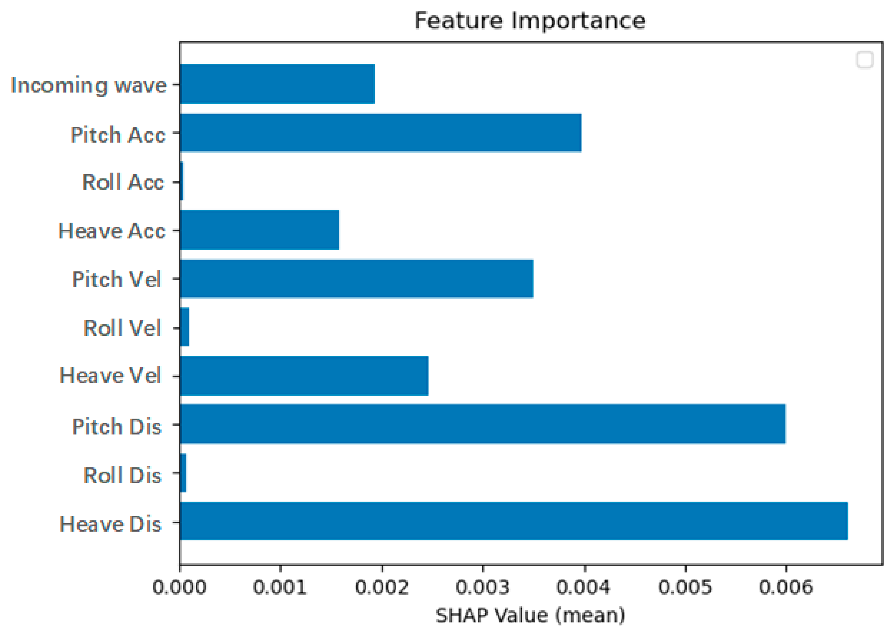
The global interpretation of feature influence is primarily conducted through SHAP Value analysis, which assesses the significance and polarity of each feature’s impact on the model’s predicted values. The SHAP Value for each feature is derived from the average absolute value of Shapley Values across all samples. The ranking of feature importance and the polarity of the impact of features on the model’s predicted values are shown in Figure 12, Figure 13 and Figure 14. In summary, by calculating the cumulative SHAP values for each input feature under sea states four, five, and six, and computing the sum of the absolute SHAP values for these features, we have obtained a comparison of the total SHAP values for all features, which is presented in the table below. The sum of the SHAP values for the selected features accounts for 75% of the total SHAP values for all features. The table that follows provides a summary of the sensitivity analysis results for all cases. Considering various situations, we ultimately selected heave displacement, pitch displacement, pitch velocity, pitch acceleration, and incoming wave height as the input variables.

5.3. Verification of Sensitivity Parameter Selection

When a ship sails at sea, its attitude changes are correlated with numerous factors, and the degree of correlation differs among various dimensions. Directly utilizing the ship’s motion attitude for method training and prediction can be challenging due to the intricate conditions encountered during actual ship navigation. Therefore, a range of factors, including motion parameters and environmental parameters, must be considered as inputs for training the method. When inputting multi-dimensional ship data, it is imperative to consider not only the temporal relationships within the ship’s time series but also the spatial relationships. To validate the accuracy of the features selected in this paper, the experimental results obtained using the CNN-BiLSTM-Attention method, after incorporating various features, are presented in

Table 13. Model validation results under sea state four conditions.

Evaluation Metrics	Full Input	Optimized Input
MAPE (%)	20.6654	9.0017
APE (%)	2.3391	1.9763
RMSE (%)	0.0049	0.0028

,

Table 14. Sensitivity analysis of input validation for sea state five conditions.

Evaluation Metrics	Full Input	Optimized Input
MAPE (%)	13.7541	11.4060
APE (%)	12.1682	0.4413
RMSE	0.0354	0.0296

and

Table 15. Sensitivity analysis of input validation for sea state six conditions.

Evaluation Metrics	Full Input	Optimized Input
MAPE (%)	55.1988	9.2711
APE (%)	8.5259	3.9324
RMSE	0.0741	0.0578

and Figure 15, Figure 16 and Figure 17. Model validation results under sea state four conditions. This study investigates the effect of multi-feature input versus single-feature input on the accuracy of the method. Specifically, heave motion in head seas under sea state four conditions is utilized as input data to train an LSTM method for forecasting ship heave motion. This study reveals that the prediction accuracy decreases and the errors increase when other features are added, thereby confirming the relative accuracy of the features selected in this paper.

This chapter conducts a sensitivity analysis to assess the impact of various input features on the forecasting outcomes of ship heave motion. The SHAP (Shapley Additive explanations) method is employed to quantify the contribution of each input feature to the method’s predictions. This analysis includes a comprehensive set of features, such as roll, pitch, heave, roll angular velocity, pitch angular velocity, heave velocity, roll angular acceleration, pitch angular acceleration, heave acceleration, and the height of incoming waves at the 5 m position at the bow. By comparing the sensitivity analysis results across various sea conditions, heave displacement, pitch displacement, pitch velocity, pitch acceleration, and incoming wave height have been identified as the pivotal input features. The inclusion of these features not only improves the method’s predictive accuracy but also enhances its adaptability to variations in input variables, resulting in more reliable forecasting outcomes. The sensitivity analysis results demonstrate that the selected features can effectively capture the primary factors influencing ship heave motion, further confirming the effectiveness and robustness of the CNN-BiLSTM-Attention method in ship motion forecasting.

6. Method Validation

To validate the effectiveness of the aforementioned method, the described procedure and parameters were applied to a model of a container ship in head seas at 150° with a speed of 20 knots, simulating sea state four conditions. Sensitivity analysis was conducted on various parameters, including roll, pitch, heave, roll angular velocity, pitch angular velocity, heave velocity, roll angular acceleration, pitch angular acceleration, heave acceleration, and wave height measured 5 m ahead of the bow. By comparing the sensitivity analysis results across different sea conditions, heave displacement, pitch velocity, pitch acceleration, and incoming wave were ultimately identified as the most sensitive parameters. The results of the sensitivity analysis are shown in Figure 18. Sensitivity analysis summary of heave motion prediction results under sea state four conditions.

Table 16. Sensitivity analysis statistics table for prediction results of heave motion under sea state four conditions.

Input Parameters	Shap	Percentage
Heave Dis	0.00346692	14.38%
Roll Dis	0.00096211	3.99%
Pitch Dis	0.00469859	19.49%
Heave Vel	0.00204863	8.50%
Roll Vel	0.0006967	2.89%
Pitch Vel	0.00248407	10.30%
Heave Acc	0.00176664	7.33%
Roll Acc	0.00284072	11.78%
Pitch Acc	0.00290292	12.04%
Incoming wave	0.00224354	9.31%

and Figure 18. Considering the impact of both the full set of input features and the post-optimization features on the experimental results of the CNN-BiLSTM-Attention method, the final results for sea state four are presented in

Table 17. Comparison and validation results of the sea state four conditions.

Evaluation Metrics	Full Input	Optimized Input
MAPE (%)	32.3550	5.0210
APE (%)	16.0276	7.6314
RMSE (%)	0.0345	0.0057

and Figure 19.

As shown in Table 17 and Figure 19, the optimized model has achieved reductions of 84.48% in MAPE (Mean Absolute Percentage Error), 52.39% in APE (Average Percentage Error), and 83.48% in RMSE (Root Mean Square Error). The feasibility of this method for forecasting heave motion under complex sea conditions has been confirmed.

7. Conclusions

In this paper, we propose a CNN-BiLSTM-Attention hybrid neural network method for predicting the heave motion of ships under complex sea conditions. This model leverages the image feature extraction capabilities of CNNs, the sequential data analysis capabilities of BiLSTMs, and the Attention mechanism to enhance the model’s focus on important features. To evaluate the predictive power of this model, we used a KCS ship model navigating at 20 knots with a heading of 180° as an example. Our results revealed that traditional models, such as LSTM and Attention methods, suffer from insufficient feature extraction and significant prediction fluctuations at extreme points. By contrast, the proposed CNN-BiLSTM-Attention method better extracts feature information, leading to more accurate predictions of ship heave motion under complex sea conditions. Across different sea conditions, the CNN-BiLSTM-Attention model significantly outperforms traditional LSTM and Attention models in terms of predictive accuracy.

To further improve the accuracy of ship heave motion forecasting, this study examines the impact of input sequence length and conducts a sensitivity analysis on the forecasting accuracy of the CNN-BiLSTM-Attention hybrid neural network model. The optimal input sequence length was determined, and through sensitivity analysis, key input features such as heave displacement, pitch angle, pitch acceleration, and wave height at the bow were identified. The selection of these features further enhanced the model’s predictive performance. Additionally, the aforementioned process was applied to a KCS ship model navigating at 20 knots with a heading of 150°, confirming the effectiveness of this method for ship heave motion prediction under complex sea conditions.

The precise results of the CNN-BiLSTM-Attention model demonstrate that the proposed method for ship heave motion prediction is a promising tool for ship heave motion prediction. However, further validation and optimization of the model in practical applications are necessary to ensure its generalization capability and robustness across a broader range of sea conditions and ship types.